Microsoft Office 2016 At Work For Dummies (2016)
Chapter 8
Creating Excel Formulas and Functions
In This Chapter
![]() Writing basic formulas
Writing basic formulas
![]() Copying and moving formulas
Copying and moving formulas
![]() Inserting functions
Inserting functions
![]() Showing the current date or time with a function
Showing the current date or time with a function
![]() Calculating loan terms
Calculating loan terms
![]() Evaluating a condition with an IF function
Evaluating a condition with an IF function
![]() Referring to named ranges
Referring to named ranges
![]() Using the Quick Analysis feature
Using the Quick Analysis feature
Math. Excel is really good at it, and it’s what makes Excel more than just data storage. Even if you hated math in school, you might still like Excel because it does the math for you.
In Excel, you can write math formulas that perform calculations on the values in various cells, and then, if those values change later, you can see the formula results update automatically. You can also use built-in functions to handle more complex math activities than you might be able to set up yourself with formulas. This capability makes it possible to build complex worksheets that calculate loan rates and payments, keep track of your bank accounts, and much more.
In this chapter, I show you how to construct formulas and functions in Excel, how to move and copy formulas and functions (there’s a trick to it), and how to use functions to create handy financial spreadsheets.
Write basic formulas
A formula is a math calculation, like 2+2 or 3*(4+1). In Excel, a formula can perform calculations with fixed numbers or cell contents.
In Excel, formulas are different from regular text in two ways:
· Formulas begin with an equal sign, like this: =2+2.
· Formulas don’t contain text (except for function names and cell references). They contain only symbols that are allowed in math formulas, such as parentheses, commas, and decimal points.
 Excel also has an advantage over some basic calculators (including the one in Windows): It easily does exponentiation. For example, if you want to calculate 5 to the 8th power, you would write it in Excel as =5^8.
Create formulas that calculate numeric values
To create a basic formula that performs math calculations on numbers:
![]() In the desired cell, begin typing the formula to create, starting with an = sign.
In the desired cell, begin typing the formula to create, starting with an = sign.
![]() Type the formula to calculate. Use these math operators:
Type the formula to calculate. Use these math operators:
· + for addition
· - for subtraction
· * for multiplication
· / for division
· ^ for exponentiation
3. Press Enter. The formula result appears in the cell, and the cell cursor moves down into the next row.
![]() (Optional) To see the formula in the cell, click the cell. Its formula appears in the formula bar.
(Optional) To see the formula in the cell, click the cell. Its formula appears in the formula bar.
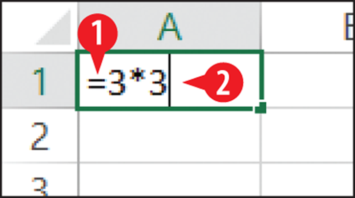
Figure 8-1: Type a formula into a cell.
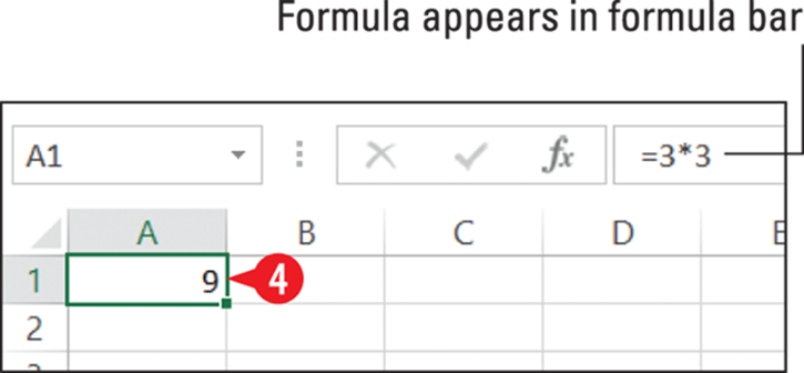
Figure 8-2: The formula result appears in the cell and the formula itself appears in the formula bar.
Control the order of math precedence
Just as in basic math, formulas are calculated by an order of precedence. Table 8-1 lists the order.
Table 8-1 Order of Precedence in a Formula
|
Order |
Item |
Example |
|
1 |
Anything in parentheses |
=2*(2+1) |
|
2 |
Exponentiation |
=2^3 |
|
3 |
Multiplication and division |
=1+2*2 |
|
4 |
Addition and subtraction |
=10-4 |
Here are a few additional examples. Work through them yourself and see if you come up with the same results; if you do, then you understand order of precedence.
· 3*3+4/2 = 11
· 3*(3+4)/2= 10.5
· 3*3+4^2= 25
Reference other cells in a formula
One of Excel’s best features is that it can reference cells in formulas. When a cell is referenced in a formula, whatever value it contains is used in the formula. When the value changes, the result of the formula changes too.
To reference another cell in a formula:
![]() Begin typing the formula to create, starting with an = sign.
Begin typing the formula to create, starting with an = sign.
2. When you need to reference another cell, do either of the following:
![]() Type the cell’s address directly into the formula (for example, A1).
Type the cell’s address directly into the formula (for example, A1).
![]() Click the cell to fill in its address in the formula being typed.
Click the cell to fill in its address in the formula being typed.
3. Continue creating the formula normally, adding numbers and math operators as needed. When you are finished, press Enter.
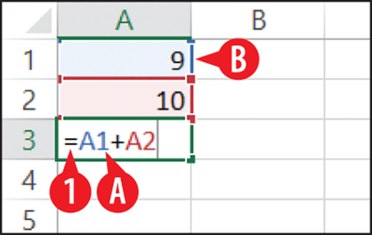
Figure 8-3: Type a formula that includes references to other cells by their column letter and row number.
Reference cells on other worksheets
When referring to a cell on the same sheet, you can simply use its column and row: A1, B1, and so on. However, when referring to a cell on a different sheet, you have to include the sheet name in the formula.
The syntax for doing this is to list the sheet name in single quotes, followed by an exclamation point, followed by the cell reference, like this:
='Sheet1'!A2
You can also select cells on another sheet by first clicking the sheet tab and then the desired cell as you are creating the formula, as in the following steps:
![]() Begin typing the formula to create, starting with an = sign.
Begin typing the formula to create, starting with an = sign.
![]() When you need to reference a cell on another sheet, click the worksheet’s tab.
When you need to reference a cell on another sheet, click the worksheet’s tab.
![]() Click the desired cell on that sheet.
Click the desired cell on that sheet.
4. Press Enter to return to the sheet containing the formula you began in step 1. Excel assumes that the formula is complete at this point and moves out of that cell.
5. If the formula is not yet complete, click the cell containing the formula and edit it in the formula bar.
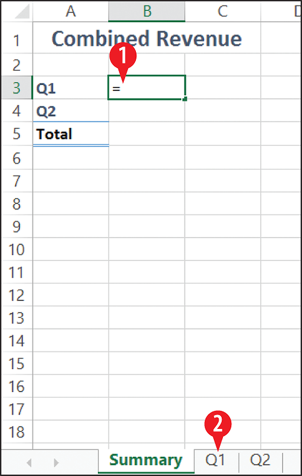
Figure 8-4: Click a tab while typing a formula to reference a cell on that sheet.
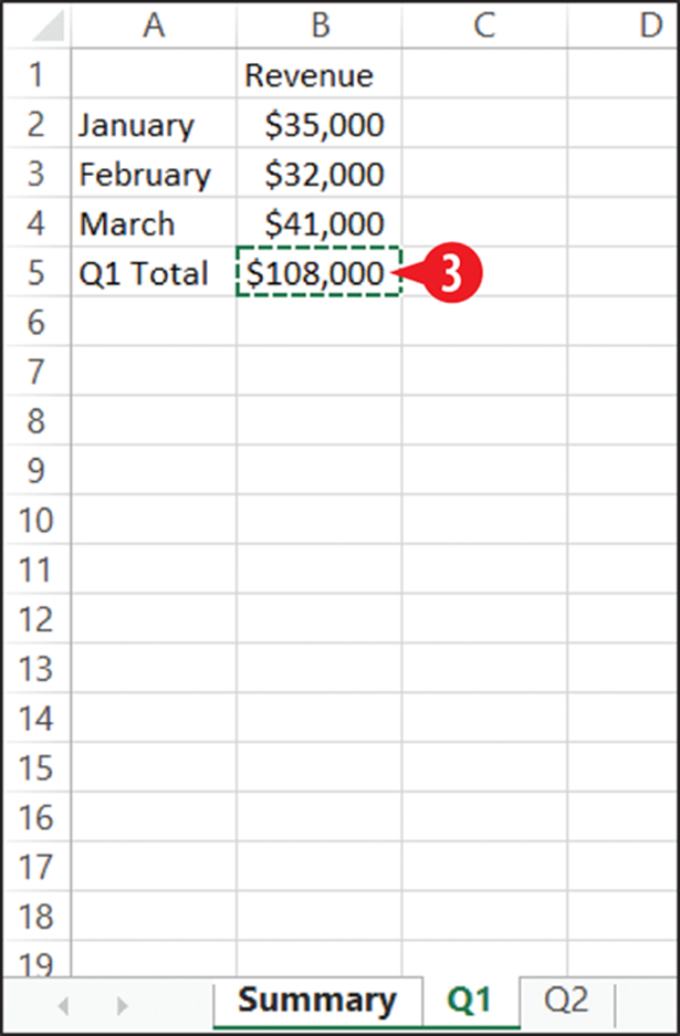
Figure 8-5: Click the desired cell to reference and press Enter.
 As you may have noticed in the preceding steps, one of the drawbacks to selecting a cell this way is that Excel ends the formula after you select it. It’s not a big deal to edit the formula, but if you would prefer to not have to do so, you can use the typing method instead of the selecting method.
Copy and move formulas
In Chapter 7, you learn how to move and copy text and numbers between cells, but when it comes to copying formulas, beware of a few gotchas. The following sections explain relative and absolute referencing in formulas and how you can use them to get the results you want when you copy.
Refer to cells with relative referencing
When you move or copy a formula, Excel automatically changes the cell references to work with the new location. That’s because, by default, cell references in formulas are relative references.
For example, in Figure 8-6, suppose you wanted to copy the formula from F2 into F3. The new formula in F3 should refer to values in row 3, not to row 2; otherwise the formula wouldn’t make much sense. So, when F2’s formula is copied to F3, it becomes =B3+C3+D3+E3there.
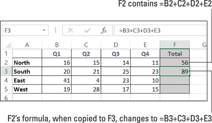
Figure 8-6: Most of the time when you copy a formula, you want its cell references to change.
You don’t have to do anything special to move copy with relative referencing. It’s the default when you move or copy. See Chapter 7.
Refer to cells with absolute referencing
You might not always want the cell references in a formula to change when you move or copy it. In other words, you want an absolute reference to that cell. To make a reference absolute, you add dollar signs before the column letter and before the row number. So, for example, an absolute reference to cell B1 would be =$B$1.
Figure 8-7 shows an example scenario in which an absolute reference would be appropriate.
![]() Cell B4 contains the formula =A4*$B$1. This calculates the tax on the amount in A4, where the tax rate appears in B1.
Cell B4 contains the formula =A4*$B$1. This calculates the tax on the amount in A4, where the tax rate appears in B1.
![]() If you copy this formula to the range B5:B17, you want the reference to the purchase price to change for each row (A5, A6, A7, and so on).
If you copy this formula to the range B5:B17, you want the reference to the purchase price to change for each row (A5, A6, A7, and so on).
![]() However, you want the reference to the tax rate to stay the same for each row.
However, you want the reference to the tax rate to stay the same for each row.
The dollar signs in the reference $B$1 ensure that that cell reference will remain static when copied.
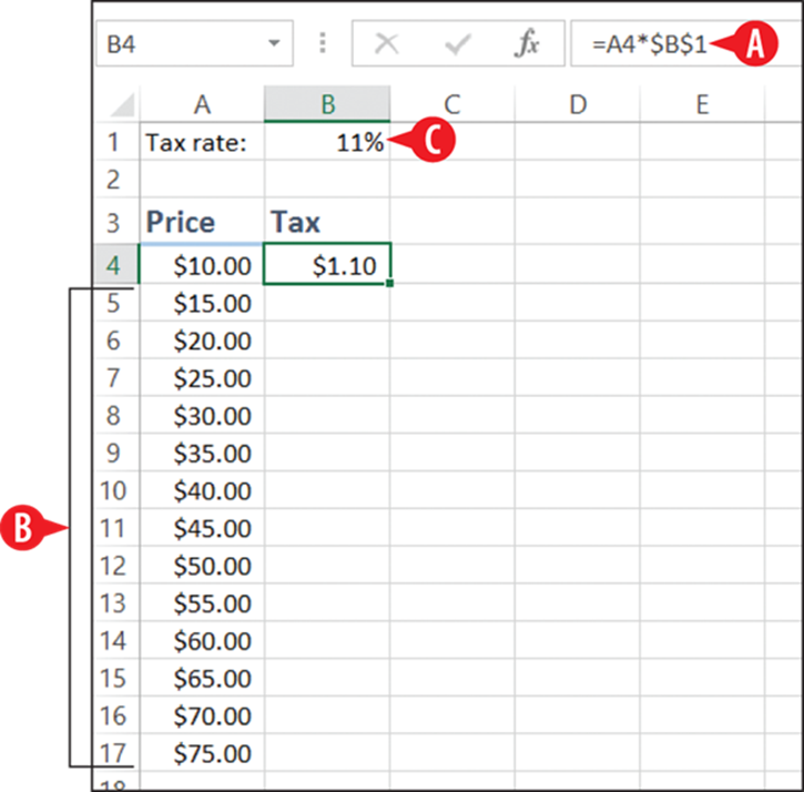
Figure 8-7: An absolute reference ensures the cell reference will not change when copied.
If you want to lock down only one dimension of the cell reference, you can place a dollar sign before only the column or only the row. For example, =$C1 would make only the column letter fixed, and =C$1 would make only the row number fixed. This is called a mixed reference.
To create an absolute or mixed reference, you can type the dollar signs directly into the cell where they are needed. Alternatively you can press F4 to cycle through all the available combinations of relative, mixed, and absolute references.
Insert functions
In Excel, a function refers to a named type of calculation. Functions can greatly reduce the amount of typing you have to do to create a particular result.
![]() For example, instead of using the =B2+B3+B4+B5+B6+B7+B8+B9+B10+B11 formula, you could use the SUM function like this: =SUM(B2:B11).
For example, instead of using the =B2+B3+B4+B5+B6+B7+B8+B9+B10+B11 formula, you could use the SUM function like this: =SUM(B2:B11).
![]() With a function, you can represent a range with the upper-left corner’s cell reference, a colon, and the lower-right corner’s cell reference. In the case of B2:B11, there is only one column, so the upper-left corner is cell B2, and the lower-right corner is cell B11.
With a function, you can represent a range with the upper-left corner’s cell reference, a colon, and the lower-right corner’s cell reference. In the case of B2:B11, there is only one column, so the upper-left corner is cell B2, and the lower-right corner is cell B11.
Range references cannot be used in simple formulas — only in functions. For example, =A6:A9 would be invalid as a formula because no math operation is specified in it. You can’t insert math operators within a range. To use ranges in a calculation, you must use a function.
An argument is a placeholder for a number, text string, or cell reference. Each function has one or more arguments, along with its own rules about how many required and optional arguments there are and what they represent. For example, the SUM function requires at least one argument: a range of cells. So, in the preceding example, B2:B11 is the argument. The arguments for a function are enclosed in a set of parentheses.
![]() You don’t have to memorize the sequence of arguments (the syntax) for each function. Excel prompts you for them. When you type a function directly into a cell, a ScreenTip prompts you for that function’s arguments.
You don’t have to memorize the sequence of arguments (the syntax) for each function. Excel prompts you for them. When you type a function directly into a cell, a ScreenTip prompts you for that function’s arguments.
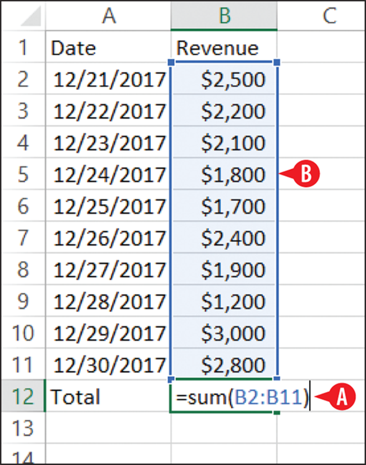
Figure 8-8: You can specify a range as one of the function’s arguments.
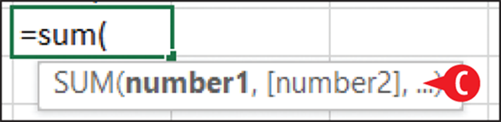
Figure 8-9: Excel prompts you for arguments when you type a function.
Use the SUM function
The SUM function is by far the most popular function; it sums (that is, adds) a data range consisting of one or more cells, like this:
=SUM(D12:D15)
You don’t have to use a range in a SUM function; you can specify the individual cell addresses if you want. Separate them by commas, like this:
=SUM(D12, D13, D14, D15)
If the data range is not a contiguous block, you need to specify the individual cells that are outside the block. The main block is one argument, and each individual other cell is an additional argument, like this:
=SUM(D12:D15, E22)
The SUM function is so frequently used that it has its own button on the Home tab, in the Editing group. Here’s how to use it.
![]() Select the cell into which you want to insert the SUM function.
Select the cell into which you want to insert the SUM function.
![]() On the Home tab, click Sum.
On the Home tab, click Sum.
![]() The SUM function is placed in the cell.
The SUM function is placed in the cell.
![]() Excel attempts to guess the range you want to sum and places a dashed outline around it.
Excel attempts to guess the range you want to sum and places a dashed outline around it.
![]() It also fills the range into the SUM function’s argument. The range is highlighted so it can be easily removed.
It also fills the range into the SUM function’s argument. The range is highlighted so it can be easily removed.
3A. If the range is correctly selected, press Enter to accept it.
OR
3B. Drag across the correct range to make a different selection and then press Enter.
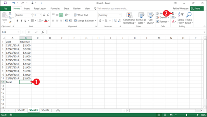
Figure 8-10: Select the cell to hold the function and then click Sum.
When you press Enter to complete a function, as in step 3, Excel automatically adds a closing parenthesis to the function if there was not one already entered. You do not have to worry about typing one.
Use AVERAGE, COUNT, MAX, and MIN functions
Perhaps you noticed that the Sum button on the Home tab has an arrow on it. Click the arrow for a list. (See ![]() in Figure 8-12.) From this list you can select one of several other common functions to use instead of SUM:
in Figure 8-12.) From this list you can select one of several other common functions to use instead of SUM:
![]() Average: Provides the average of the numeric values within the selected range. Ignores blank and non-numeric values
Average: Provides the average of the numeric values within the selected range. Ignores blank and non-numeric values
![]() Count Numbers: Counts the number of cells within the selected range that contain numeric values
Count Numbers: Counts the number of cells within the selected range that contain numeric values
![]() Max: Finds and returns the largest numeric value within the selected range
Max: Finds and returns the largest numeric value within the selected range
![]() Min: Finds and returns the smallest numeric value within the selected range
Min: Finds and returns the smallest numeric value within the selected range
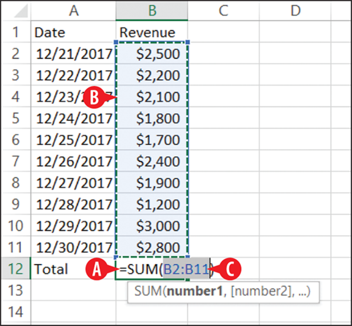
Figure 8-11: Excel tries to complete the function for you.
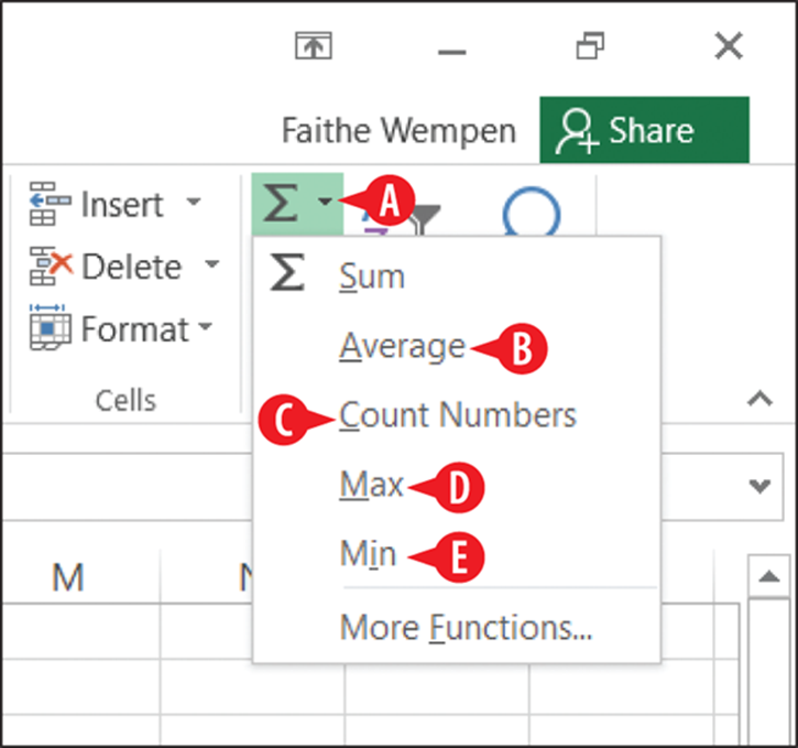
Figure 8-12: You can select other common functions from the Sum button’s menu.
Find and insert a function
Typing a function and its arguments directly into a cell works fine if you happen to know the function you want and its arguments. Many times, though, you may not know these details. In those cases, the Insert Function feature can help you.
Insert Function enables you to pick a function from a list based on descriptive keywords. After you make your selection, it provides fill-in-the-blank prompts for the arguments.
To insert a function:
![]() Select the cell in which to insert the function.
Select the cell in which to insert the function.
![]() On the formula bar, click the Insert Function button to open the Insert Function dialog box.
On the formula bar, click the Insert Function button to open the Insert Function dialog box.
![]() In the Search for a function describe what you want to do.
In the Search for a function describe what you want to do.
![]() In the Select a function box, click a function and then read about it below the list.
In the Select a function box, click a function and then read about it below the list.
![]() When the appropriate function is selected, click OK.
When the appropriate function is selected, click OK.
6. In the Function Arguments dialog box, type the number or enter the cell reference for each argument. Here are some things to remember about this dialog box:
![]() You can type directly into any of the argument text boxes.
You can type directly into any of the argument text boxes.
![]() You can click in an argument’s box and then click a cell on the worksheet behind the dialog box to fill in that cell reference.
You can click in an argument’s box and then click a cell on the worksheet behind the dialog box to fill in that cell reference.
![]() You can click the Collapse Dialog button for any argument to temporarily shrink the dialog box so you can see which cell you want to choose.
You can click the Collapse Dialog button for any argument to temporarily shrink the dialog box so you can see which cell you want to choose.
![]() Arguments in bold are required.
Arguments in bold are required.
![]() Arguments that are not in bold are optional.
Arguments that are not in bold are optional.
![]() The Formula Result area previews the formula’s result.
The Formula Result area previews the formula’s result.
![]() Click OK to complete the function.
Click OK to complete the function.
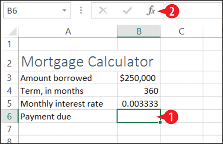
Figure 8-13: Click Insert Function on the formula bar.
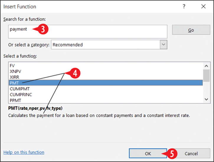
Figure 8-14: Describe the function’s purpose, and then browse the list to find the one you want.
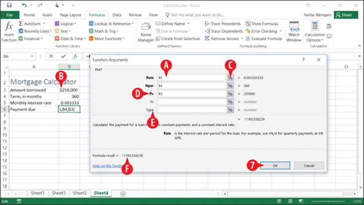
Figure 8-15: Fill in the arguments for the chosen function.
Choose from the Function Library
Once you become familiar with the names of Excel’s most common functions, you will not need to look them up every time you need one, as you did in the previous section. Instead you can shortcut the process, either by typing them directly into the cell or by choosing them from the Function Library group on the Formulas tab.
The Formulas tab’s Library group organizes functions by their general purpose. There is a separate drop-down list button for each category. There are also extra buttons for AutoSum, which is the same as the Sum button on the Home tab, and Recently Used.
To select a function from the library, follow these steps:
1. Select the cell in which to insert the function.
![]() On the Formulas tab, click the button for the category of function you want.
On the Formulas tab, click the button for the category of function you want.
![]() Scroll through the list and click the desired function.
Scroll through the list and click the desired function.
You can point at a function on the list to see a pop-up box describing it. (See ![]() in Figure 8-16.)
in Figure 8-16.)
4. Pick up the steps in the preceding section, “Find and insert a function,” at step 6 to complete the function.
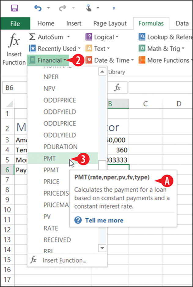
Figure 8-16: Choose the desired function from the category list.
Show the current date or time with a function
You can use functions to show the current date or time in a cell and have that value be updated automatically every time you open the worksheet. (You can also update the field manually any time by pressing F9 or choosing Formulas ⇒ Calculate Now.) The functions to do this are
· NOW: Reports the current date and time
· TODAY: Reports the current date
Even though neither uses any arguments, you still have to include the parentheses, so they look like this when you use them:
=NOW( )
=TODAY( )
If you want a different format than the default for either of those results, you’ll need to apply a different number format to the cell. Here’s how:
![]() With the cell selected that contains the function, click the dialog box launcher for the Number group on the Home tab.
With the cell selected that contains the function, click the dialog box launcher for the Number group on the Home tab.
![]() In the Format Cells dialog box, in the Category list, click either Date or Time, whichever you want.
In the Format Cells dialog box, in the Category list, click either Date or Time, whichever you want.
![]() Select the desired format from the Type list.
Select the desired format from the Type list.
![]() Click OK.
Click OK.
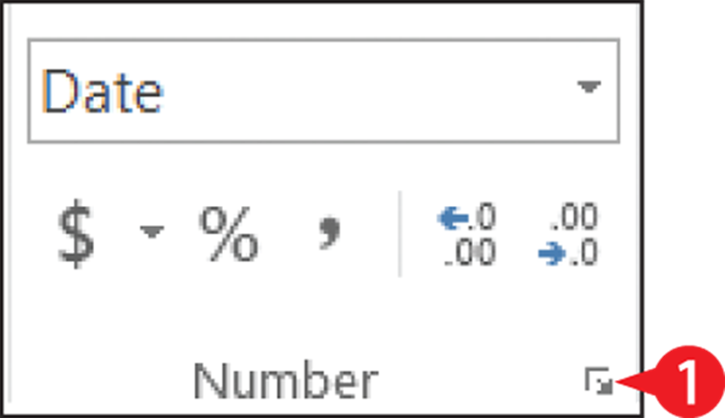
Figure 8-17: Click the dialog box launcher for the Number group.
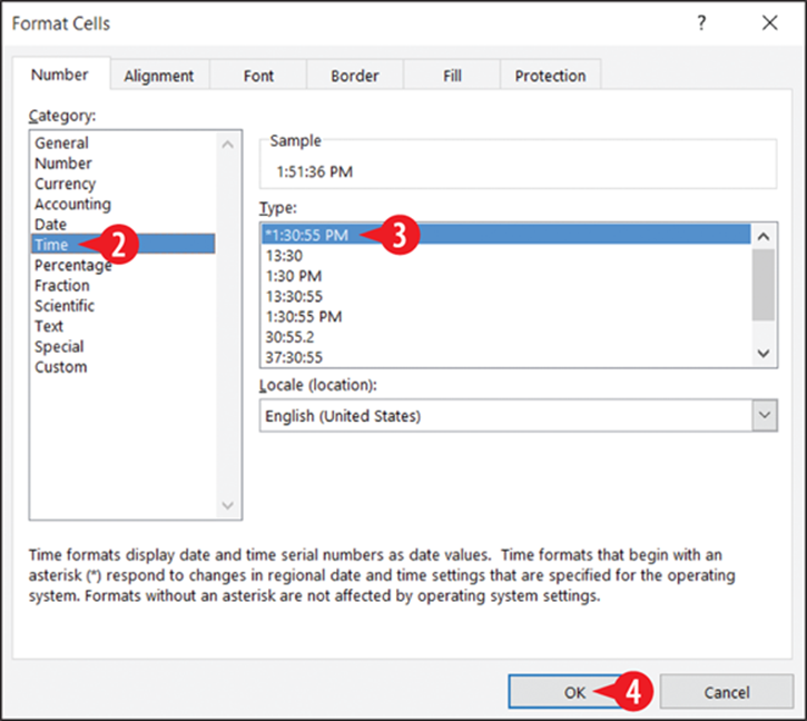
Figure 8-18: Select a specific date or time format.
You can combine the NOW or TODAY function with a formula to get results that are in the past or future. For example, =TODAY( )+7 returns the date that is 7 days in the future. Use decimal points to indicate times. For example, =NOW( )-0.5 returns the time that is 12 hours (50 percent of one day) in the past.
There are many other date and time functions available. Check out the functions on the Date & Time button’s menu on the Formulas tab.
Calculate loan terms
One of the most common calculation tasks in Excel is to determine the terms of a loan. There is a set of functions designed specifically for this task. Each function finds a different part of the loan equation, given the other parts:
· PV: Short for present value; finds the amount of the loan
· NPER: Short for number of periods; finds the number of payments (the length of the loan)
· RATE: Finds the interest rate per period
· PMT: Finds the amount of the payment per period
Each of those functions uses the other three pieces of information as its required arguments. For example, the arguments for PV are rate, nper, and pmt.
So, let’s say, for example, that you want to know the length of a loan in which you borrow $20,000 at 5 percent interest per year (0.417 percent per month) if you make a monthly payment of $350. You can use the NPER function to figure that out. Here’s how:
![]() In Excel, create the labels needed for the structure of the worksheet, as shown in Figure 8-19. Fill in the information you already know about the loan.
In Excel, create the labels needed for the structure of the worksheet, as shown in Figure 8-19. Fill in the information you already know about the loan.
![]() Type =NPER( into the cell where the function should be placed.
Type =NPER( into the cell where the function should be placed.
A ScreenTip reminds you of the arguments to use and their proper order. (See ![]() in Figure 8-20.)
in Figure 8-20.)
![]() Click or type the cell that contains the interest rate and then type a comma.
Click or type the cell that contains the interest rate and then type a comma.
![]() Click or type the cell that contains the payment amount, and then type a comma.
Click or type the cell that contains the payment amount, and then type a comma.
![]() Click or type the cell that contains the loan amount, and then press Enter to complete the formula. The closing parenthesis is automatically added for you. If you do the example correctly, the loan term will show as -58.95187.
Click or type the cell that contains the loan amount, and then press Enter to complete the formula. The closing parenthesis is automatically added for you. If you do the example correctly, the loan term will show as -58.95187.
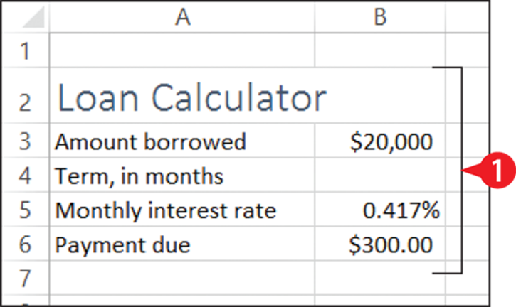
Figure 8-19: Create the structure of the worksheet, including the descriptive labels and any numbers that you already know.
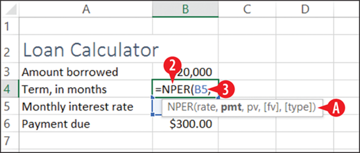
Figure 8-20: Begin entering the function and its arguments.
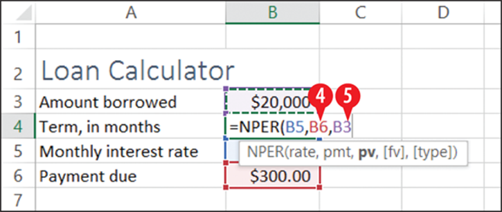
Figure 8-21: Add the remaining arguments, separating them with commas.
Besides these four simple functions, there are dozens of other financial functions available in Excel. For example, IPMT is like PMT except it returns only the amount of interest in the payment, and PPMT returns only the amount of principal. Explore the functions on the Financial button’s menu on the Formulas tab on your own.
The result of the calculation will be negative if the present value (the loan amount) is a positive number. If you want the term to show as a positive number, change the amount borrowed to a negative number, or enclose the function within the ABS function (absolute value), like this: =ABS(NPER(B5,B6,B3)). ABS is short for absolute value.
Since the number of payments must be a whole number, you might choose to use the ROUNDUP function to round that value up to the nearest whole. The ROUNDUP function has two arguments: the number to be rounded and a number of decimal places. For a whole number, use 0 for the second argument. The finished formula would then look like this: =ROUNDUP(ABS(NPER(B5,B6,B3)),0).
Perform math calculations
Technically, all formulas perform math calculations, but there’s a specific category of functions called Math & Trig for functions that deal directly with familiar math calculations like finding the square root (SQRT), tangent (TAN), sine (SIN), or cosine (COS) of a number. TheABS and ROUNDUP functions I mentioned at the end of the previous section fall into this category also. Check out the Math & Trig category list on the Formulas tab for a complete list of math functions.
Most of the math-related functions are fairly simple, with just one or two arguments. For example, the SQRT function takes only one argument: the number to be calculated. SQRT(A1) finds the square root of the number in cell A1.
Evaluate a condition with an IF function
The IF function determines whether or not a condition is true and then performs different actions based on that answer. IF is only one of many logical functions that Excel provides; see the list on the Logical button on the Formulas tab for others. For example:
![]() Suppose a customer gets a 10 percent discount if he spends more than $50. You could use the IF function to determine whether his order amount qualifies.
Suppose a customer gets a 10 percent discount if he spends more than $50. You could use the IF function to determine whether his order amount qualifies.
An IF function typically contains three arguments: condition, value_if_true, and value_if_false. Like all arguments, they are separated by commas.
![]() The condition in this example is D5>=50. In other words, is the value in D5 greater than or equal to 50?
The condition in this example is D5>=50. In other words, is the value in D5 greater than or equal to 50?
![]() The value_if_true in this example is calculated by multiplying D5 by 0.1 (in other words, calculating 10 percent of it).
The value_if_true in this example is calculated by multiplying D5 by 0.1 (in other words, calculating 10 percent of it).
![]() The value_if_false in this example is zero (0).
The value_if_false in this example is zero (0).
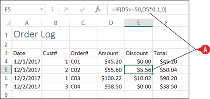
Figure 8-22: The amount of discount is determined using an IF function.
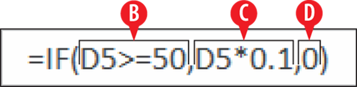
Figure 8-23: An IF function with three arguments.
The condition argument is the only required one. If you omit the value_if_true argument, the function returns 1 if the condition is true and 0 if the condition is false. If you omit the value_if_false argument, a value of 0 is assumed for it. Therefore in the above example, technically we did not have to include the value_if_false argument, since we wanted zero for it anyway.
If you want to combine a SUM operation with an IF condition, you can use the SUMIF function, which does both at once. It sums a range of data if the condition you specify in its argument is true. You’ll find it on the Math & Trig button’s list, rather than under the Logical category.
Refer to named ranges
When constructing formulas and functions, naming a range can be helpful because you can refer to that name rather than the cell addresses. Therefore you don’t have to remember the exact cell addresses, and you can construct formulas based on meaning. For example:
![]() Instead of remembering that the number of employees is stored in cell B2, you could name the cell B2 Employees.
Instead of remembering that the number of employees is stored in cell B2, you could name the cell B2 Employees.
![]() Then in a formula that used B2’s value, such as =B2*3, you could use the name instead: =Employees*3.
Then in a formula that used B2’s value, such as =B2*3, you could use the name instead: =Employees*3.
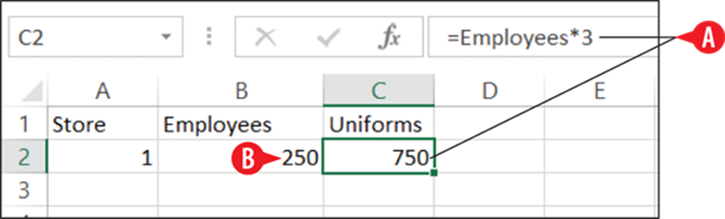
Figure 8-24: You can use range names in formulas.
You can name individual cells, as in the above example, but in some cases it may be more advantageous to name multi-cell ranges. For example, you might name multiple cells in a column that contains the same kind of information. When you then use the range name in a formula or function, Excel assumes that you mean the cell within that range that corresponds to the row or column in which you are typing:
![]() In Figure 8-25, the named range of Employees encompasses B2:B7.
In Figure 8-25, the named range of Employees encompasses B2:B7.
![]() The same formula is used in every cell in column C: =Employees*3.
The same formula is used in every cell in column C: =Employees*3.
![]() In each row, Excel assumes that you mean the cell in that same row.
In each row, Excel assumes that you mean the cell in that same row.
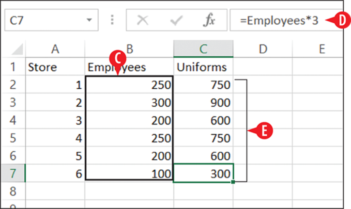
Figure 8-25: When a multi-cell range is named, references to that range are relative to the cell in which the formula is entered.
Excel is rather intelligent about deducing what you mean when you refer to named ranges. When you refer to a range in a calculation like the one shown in Figure 8-25, the reference is to an individual cell in the range. However, if you use the range name in a formula where it makes sense to be referring to the entire range, Excel does so.
For example, =SUM(Employees) would return the sum of all values within that range. (See ![]() in Figure 8-26.)
in Figure 8-26.)
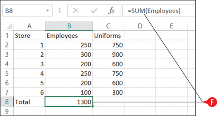
Figure 8-26: When you refer to a multi-cell range in a context that infers the entire range, Excel interprets it that way.
You can name a range in three ways, and each has its pros and cons.
Create range names by selection
If default names are okay to use, you may find automatic naming useful. With this method, Excel chooses the name for you based on text labels it finds in adjacent cells (above or to the left of the current cells). This method is fast and easy, and it works well when you have to create a lot of names at once and when the cells are well labeled with adjacent text:
![]() Select the range to name. If you want to create multiple named ranges, each referring to a different column or row, select the entire range, including the cells containing the names to use.
Select the range to name. If you want to create multiple named ranges, each referring to a different column or row, select the entire range, including the cells containing the names to use.
![]() From the Formulas tab, click Create from Selection.
From the Formulas tab, click Create from Selection.
![]() In the Create Names from Selection dialog box, mark or clear check boxes as needed to indicate where the labels are.
In the Create Names from Selection dialog box, mark or clear check boxes as needed to indicate where the labels are.
![]() Click OK. The range names are created.
Click OK. The range names are created.
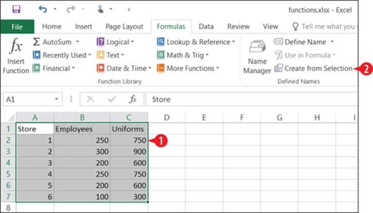
Figure 8-27: Allow Excel to automatically create ranges with names defined by labels in adjacent cells.
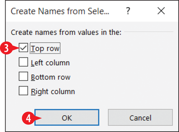
Figure 8-28: Confirm that Excel has correctly guessed where the labels are.
If you aren’t sure if the ranges were correctly created, click the Name Manager button on the Formulas tab to see a list of all named ranges and their definitions.
Create range names using the Name box
With this fast and easy method, you get to choose the name yourself. However, you have to do each range separately; you can’t do a big batch at a time:
![]() Select the cells to include in the named range. Make sure that you select only the cells that contain actual data, not the cell containing text (like the column header).
Select the cells to include in the named range. Make sure that you select only the cells that contain actual data, not the cell containing text (like the column header).
![]() Click in the Name box and type the new range name.
Click in the Name box and type the new range name.
3. Press Enter.
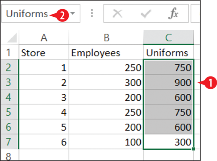
Figure 8-29: Type a range name into the Name box.
Create range names using Define Name
If you want to more precisely control the options for the name, you can use the Define Name command. This method opens a dialog box from which you can specify the name, the scope, and any comments you might want to include:
![]() Select the cells to include in the named range. Make sure that you select only the cells that contain actual data, not the cell containing text (like the column header).
Select the cells to include in the named range. Make sure that you select only the cells that contain actual data, not the cell containing text (like the column header).
![]() On the Formulas tab, click Define Name.
On the Formulas tab, click Define Name.
![]() In the New Name dialog box, type the desired name in the Name box.
In the New Name dialog box, type the desired name in the Name box.
![]() (Optional) To limit the scope of the name to just the active worksheet, change the Scope setting to a particular sheet (such as Sheet1).
(Optional) To limit the scope of the name to just the active worksheet, change the Scope setting to a particular sheet (such as Sheet1).
![]() (Optional) Type any comments in the Comment box. This can help you remember why you created the range.
(Optional) Type any comments in the Comment box. This can help you remember why you created the range.
![]() Click OK.
Click OK.
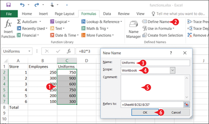
Figure 8-30: Define a range using the Define Name command.
Use Quick Analysis features
Here are some points to keep in mind about Quick Analysis:
![]() When you select a range of cells, a small icon appears in the lower right corner of the selected area. This is the Quick Analysis icon, and clicking it opens a panel containing shortcuts to several types of common activities related to data analysis.
When you select a range of cells, a small icon appears in the lower right corner of the selected area. This is the Quick Analysis icon, and clicking it opens a panel containing shortcuts to several types of common activities related to data analysis.
![]() Click on the five headings to see the shortcuts available in that category. Then hover over one of the icons in that category to see the result previewed on your worksheet.
Click on the five headings to see the shortcuts available in that category. Then hover over one of the icons in that category to see the result previewed on your worksheet.
![]() Formatting: These shortcuts point to conditional formatting options, which you will learn about in Chapter 9. For example, you could set up a range to make values under or over a certain amount appear in a different color or with a special icon adjacent.
Formatting: These shortcuts point to conditional formatting options, which you will learn about in Chapter 9. For example, you could set up a range to make values under or over a certain amount appear in a different color or with a special icon adjacent.
![]() Charts: These shortcuts generate common types of charts based on the selected data. You will learn about charts in Chapter 11.
Charts: These shortcuts generate common types of charts based on the selected data. You will learn about charts in Chapter 11.
![]() Totals: These shortcuts add the specified calculation to adjacent cells in the worksheet. For example, Sum adds a total row or column.
Totals: These shortcuts add the specified calculation to adjacent cells in the worksheet. For example, Sum adds a total row or column.
![]() Notice that there are separate icons here for rows versus columns.
Notice that there are separate icons here for rows versus columns.
![]() Notice also that in this category there are more icons than can be displayed at once, so there are right and left arrows you can click to scroll through them.
Notice also that in this category there are more icons than can be displayed at once, so there are right and left arrows you can click to scroll through them.
![]() Tables: You can convert the range to a table (covered in Chapter 10) for greater ease of analysis. You can also generate several different types of PivotTables via the shortcuts here. A PivotTable is a special view of the data that summarizes it by adding various types of calculations to it.
Tables: You can convert the range to a table (covered in Chapter 10) for greater ease of analysis. You can also generate several different types of PivotTables via the shortcuts here. A PivotTable is a special view of the data that summarizes it by adding various types of calculations to it.
![]() The PivotTable icons aren’t well differentiated, but you can point to one of the PivotTable icons to see a sample of how it will summarize the data in the selected range. If you choose one of the PivotTable views, it opens in its own separate sheet.
The PivotTable icons aren’t well differentiated, but you can point to one of the PivotTable icons to see a sample of how it will summarize the data in the selected range. If you choose one of the PivotTable views, it opens in its own separate sheet.
![]() Sparklines: Sparklines are mini-charts placed in single cells. They can summarize the trend of the data in adjacent cells. They are most relevant when the data you want to trend appears from left to right in adjacent columns.
Sparklines: Sparklines are mini-charts placed in single cells. They can summarize the trend of the data in adjacent cells. They are most relevant when the data you want to trend appears from left to right in adjacent columns.
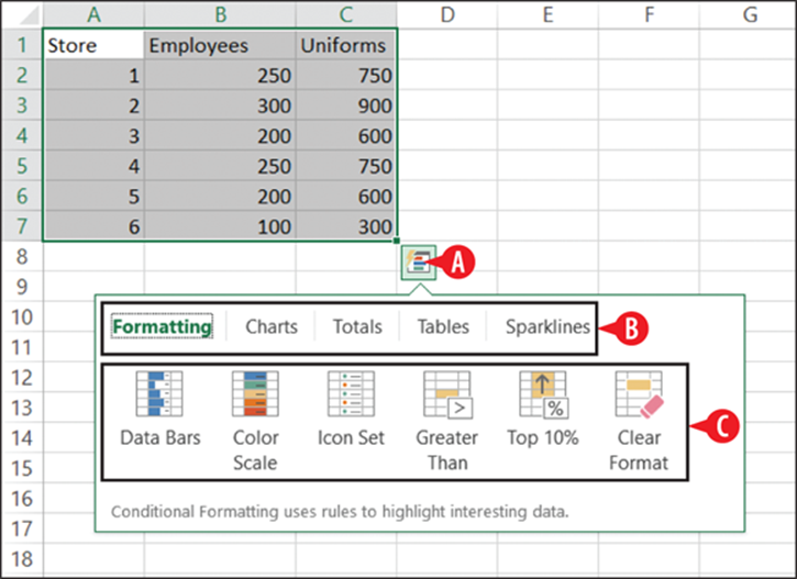
Figure 8-31: Open the Quick Analysis panel by clicking its icon. Then choose a category heading and click an icon for a command.
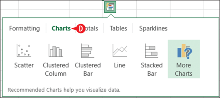
Figure 8-32: Quick Analysis offers shortcuts for creating several common chart types.
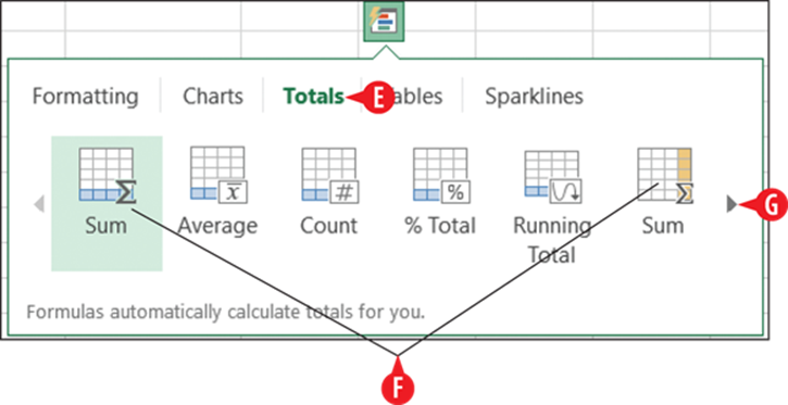
Figure 8-33: You can use Quick Analysis to add summary rows or columns.
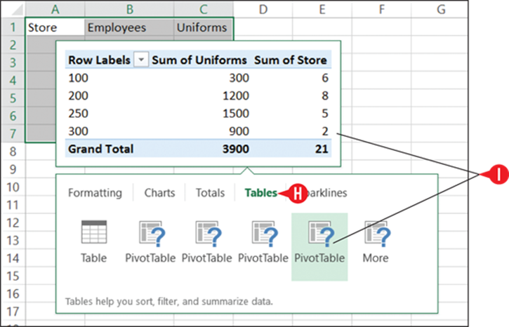
Figure 8-34: You can convert the range to a table or apply one of several PivotTable specifications.
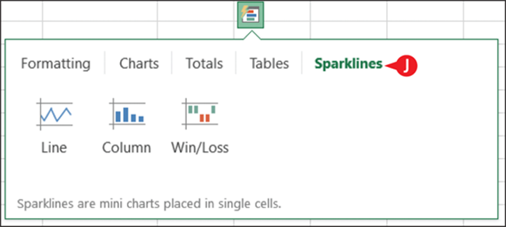
Figure 8-35: Choose Sparklines to add mini-charts that show overall trends.