T-SQL Querying (2015)
Chapter 3. Multi-table queries
This chapter’s focus is multi-table queries. It covers subqueries, table expressions, the APPLY operator, joins, and the relational operators UNION, EXCEPT, and INTERSECT.
Chapters 1 and 2 provided the foundation for the rest of the book. Chapter 1, “Logical query processing,” described the logical layer of T-SQL, and Chapter 2, “Query tuning,” described the physical layer. Each layer was described separately to emphasize its unique role—the logical layer’s role is to define meaning, and the physical layer’s role is to implement, or carry out, what the logical layer defines. The physical layer is not supposed to define meaning. Starting with this chapter, the coverage relies on the foundation provided in the previous chapters, with discussions revolving around both the logical and the physical aspects of the code.
Subqueries
Subqueries are a classic feature in SQL that you use to nest queries. Using subqueries is a convenient capability in the language when you want one query to operate on the result of another, and if you prefer not to use intermediate objects like variables for this purpose.
This section covers different aspects of subqueries. It covers self-contained versus correlated subqueries, the EXISTS predicate, and misbehaving subqueries. Subqueries can return three shapes of results: single-valued (scalar), multi-valued, and table-valued. This section covers the first two. The last type is covered later in the chapter in the “Table expressions” section.
Self-contained subqueries
A self-contained subquery is, as it sounds, independent of the outer query. In contrast, a correlated subquery has references (correlations) to columns of tables from the outer query. One of the advantages of self-contained subqueries compared to correlated ones is the ease of troubleshooting. You can always copy the inner query to a separate window and troubleshoot it independently. When you’re done troubleshooting and fixing what you need, you paste the subquery back in the host query. I’ll start by providing examples for scalar and multi-valued self-contained subqueries, and then transition to correlated ones.
The first example I’ll discuss is of a self-contained, scalar subquery. A scalar subquery returns a single value and is allowed where a single-valued expression is expected—for example, as an operand in a comparison in the WHERE clause. As an example, the following query returns customers for whom all employees in the organization handled orders:
SET NOCOUNT ON;
USE TSQLV3;
SELECT custid
FROM Sales.Orders
GROUP BY custid
HAVING COUNT(DISTINCT empid) = (SELECT COUNT(*) FROM HR.Employees);
As an aside, this query handles a simple case of what relational algebra refers to as relational division. You are dividing the set of orders in the Orders table (which connects customers and employees) by the set of employees in the Employees table, and you get back qualifying customers.
The subquery returns the count of employees in the Employees table. The outer query groups the orders from the Orders table by customer ID, and it filters only customer groups having a distinct count of employee IDs that is equal to the count of employees returned by the subquery. Obviously, this query assumes that proper referential integrity is enforced in the database, preventing an order from having an employee ID that doesn’t appear in the Employees table. The subquery returns 9 as the count of employees in the Employees table. The outer query returns customer ID 71 because that’s the only customer with orders handled by 9 distinct employees.
Note that if a scalar subquery returns an empty set, it’s converted to a NULL. If it returns more than one value, it fails at run time. Neither option is a possibility in our case, because the scalar aggregate subquery is guaranteed to return exactly one value, even if the source table is empty.
The next example is of a self-contained, multi-valued subquery. A multi-valued subquery returns multiple values in one column. It can be used where a multi-valued result is expected—for example, with the IN predicate.
The task in our example is to return orders that were placed on the last date of activity of the month. The last date of activity is not necessarily the last possible date of the month—for example, if the company doesn’t handle orders on weekends and holidays. The first step in the solution is to write a grouped query that returns the last date of activity for each year and month group, like so:
SELECT MAX(orderdate) AS lastdate
FROM Sales.Orders
GROUP BY YEAR(orderdate), MONTH(orderdate);
This query returns the following output:
lastdate
----------
2014-01-31
2014-07-31
2015-05-06
2014-04-30
2014-10-31
2015-02-27
2013-12-31
2014-05-30
2015-03-31
2013-09-30
...
This query is a bit unusual for a grouped query. Usually, you group by certain elements and return the grouped elements and aggregates. Here you group by the order year and month, and you return only the aggregate without the group elements. But if you think about it, the maximum date for a year and month group preserves within it the year and month information, so the group information isn’t really lost here.
The second and final step is to query the Orders table and filter only orders with order dates that appear in the set of dates returned by the query from the previous step. Here’s the complete solution query:
SELECT orderid, orderdate, custid, empid
FROM Sales.Orders
WHERE orderdate IN
(SELECT MAX(orderdate)
FROM Sales.Orders
GROUP BY YEAR(orderdate), MONTH(orderdate));
This query generates the following output:
orderid orderdate custid empid
----------- ---------- ----------- -----------
10269 2013-07-31 89 5
10294 2013-08-30 65 4
10317 2013-09-30 48 6
10343 2013-10-31 44 4
10368 2013-11-29 20 2
...
Correlated subqueries
Correlated subqueries have references known as correlations to columns from tables in the outer query. They tend to be trickier to troubleshoot when problems occur because you cannot run them independently. If you copy the inner query and paste it in a new window (to make it runnable), you have to substitute the correlations with constants representing sample values from your data. But then when you’re done troubleshooting and fixing what you need, you have to replace the constants back with the correlations. This makes troubleshooting correlated subqueries more complex and more prone to errors.
As the first example for a correlated subquery, consider a task similar to the last one in the previous section. The task was to return the orders that were placed on the last date of activity of the month. Our new task is to return the orders that were placed on the last date of activity of thecustomer. Seemingly, the only difference is that instead of the group being the year and month, it’s now the customer. So if you take the last query and replace the grouping set from YEAR(orderdate), MONTH(orderdate) with custid, you get the following subquery.
SELECT orderid, orderdate, custid, empid
FROM Sales.Orders
WHERE orderdate IN
(SELECT MAX(orderdate)
FROM Sales.Orders
GROUP BY custid);
However, now there is a bug in the solution. The values returned by the subquery this time don’t preserve the group (customer) information. Suppose that for customer 1 the maximum date is some d1 date, and for customer 2, the maximum date is some later d2 date; if customer 2 happens to place orders on d1, you will get those too, even though you’re not supposed to. To fix the bug, you need the inner query to operate only on the orders that were placed by the customer from the outer row. For this, you need a correlation, like so:
SELECT orderid, orderdate, custid, empid
FROM Sales.Orders AS O1
WHERE orderdate IN
(SELECT MAX(O2.orderdate)
FROM Sales.Orders AS O2
WHERE O2.custid = O1.custid
GROUP BY custid);
Now the solution is correct, but there are a couple of awkward things about it. For one, you’re filtering only one customer and also grouping by the customer, so you will get only one group. In such a case, it’s more natural to express the aggregate as a scalar aggregate without the explicit GROUP BY clause. For another, the subquery will return only one value. So, even though the IN predicate is going to work correctly, it’s more natural to use an equality operator in such a case. After applying these two changes, you get the following solution:
SELECT orderid, orderdate, custid, empid
FROM Sales.Orders AS O1
WHERE orderdate =
(SELECT MAX(O2.orderdate)
FROM Sales.Orders AS O2
WHERE O2.custid = O1.custid);
This code generates the following output:
orderid orderdate custid empid
----------- ---------- ----------- -----------
11044 2015-04-23 91 4
11005 2015-04-07 90 2
11066 2015-05-01 89 7
10935 2015-03-09 88 4
11025 2015-04-15 87 6
...
10972 2015-03-24 40 4
10973 2015-03-24 40 6
11028 2015-04-16 39 2
10933 2015-03-06 38 6
11063 2015-04-30 37 3
...
Currently, if a customer placed multiple orders on its last date of activity, the query returns all those orders. As an example, observe that the query output contains multiple orders for customer 40. Suppose you are required to return only one order per customer. In such a case, you need to define a rule for breaking the ties in the order date. For example, the rule could be to break the ties based on the maximum primary key value (order ID, in our case). In the case of the two orders that were placed by customer 40 on March 24, 2015, the maximum primary key value is 10973. Note that that’s the maximum primary key value from the customer’s orders with the maximum order date—not from all the customer’s orders.
You can use a number of methods to apply the tiebreaking logic. One method is to use a separate scalar aggregate subquery for each ordering and tiebreaking element. Here’s a query demonstrating this technique:
SELECT orderid, orderdate, custid, empid
FROM Sales.Orders AS O1
WHERE orderdate =
(SELECT MAX(orderdate)
FROM Sales.Orders AS O2
WHERE O2.custid = O1.custid)
AND orderid =
(SELECT MAX(orderid)
FROM Sales.Orders AS O2
WHERE O2.custid = O1.custid
AND O2.orderdate = O1.orderdate);
The first subquery is the same as in the solution without the tiebreaker. It’s responsible for returning the maximum order date for the outer customer. The second subquery returns the maximum order ID for the outer customer and order date. The problem with this approach is that you need as many subqueries as the number of ordering and tiebreaking elements. Each subquery needs to be correlated by all elements you correlated in the previous subqueries plus a new one. So, especially when multiple tiebreakers are involved, this solution becomes long and cumbersome.
To simplify the solution, you can collapse all subqueries into one by using TOP instead of scalar aggregates. The TOP filter has two interesting advantages in its design compared to aggregates. One advantage is that TOP can return one element while ordering by another, whereas aggregates consider the same element as both the ordering and returned element. Another advantage is that TOP can have a vector of elements defining order, whereas aggregates are limited to a single input element. These two advantages allow you to handle all ordering and tiebreaking elements in the same subquery, like so:
SELECT orderid, orderdate, custid, empid
FROM Sales.Orders AS O1
WHERE orderid =
(SELECT TOP (1) orderid
FROM Sales.Orders AS O2
WHERE O2.custid = O1.custid
ORDER BY orderdate DESC, orderid DESC);
The outer query filters only the orders where the key is equal to the key obtained by the TOP subquery representing the customer’s most recent order, with the maximum key used as a tiebreaker. To obtain the qualifying key, the subquery filters the orders for the outer customer, orders them by orderdate DESC, orderid DESC, and returns the key of the very top row.
This type of task is generally known as the top N per group task and is quite common in practice in different variations. It is discussed in a number of places in the book, with the most complete coverage conducted in Chapter 5, “TOP and OFFSET-FETCH.” Here it is discussed mainly to demonstrate subqueries.
At this point, you have a simple and intuitive solution using the TOP filter. The question is, how well does it perform? In terms of indexing guidelines, solutions for top N per group tasks usually benefit from a specific indexing pattern that I like to think of as the POC pattern. That’s an acronym for the elements involved in the task. P stands for the partitioning (the group) element, which in our case is custid. O stands for the ordering element, which in our case is orderdate DESC, orderid DESC. The PO elements make the index key list. C stands for the covered elements—namely, all remaining elements in the query that you want to include in the index to get query coverage. In our case, the C element is empid. If the index is nonclustered, you specify the C element in the index INCLUDE clause. If the index is clustered, the C element is implied. Run the following code to create a POC index to support your solution:
CREATE UNIQUE INDEX idx_poc
ON Sales.Orders(custid, orderdate DESC, orderid DESC) INCLUDE(empid);
With the index created, you get the plan shown in Figure 3-1 for the solution with the TOP subquery.
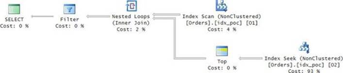
FIGURE 3-1 Plan with a seek per order.
The plan does a full scan of the POC index representing the instance O1 of the Orders table (the outer instance in the query). Then for each row from O1, the plan performs a seek in the POC index representing the instance O2 of the Orders table (the inner instance in the query). The seek reaches the beginning of the section in the leaf of the index for the current customer and scans one row to collect the key. The plan then filters only the rows from O1 where the O1 key is equal to the O2 key.
There is a certain inefficiency in this plan that can be optimized. Think about how many times the Index Seek operator is executed. Currently, you get a seek per order, but you are after only one row per customer. So a more efficient strategy is to apply a seek per customer. The denser thecustid column, the fewer seeks such a strategy would require. To make the performance discussion more concrete, suppose the data has 10,000 customers with an average of 1,000 orders each, giving you 10,000,000 orders in total. The existing plan performs 10,000,000 seeks. With three levels in the index B-tree, this translates to 30,000,000 random reads. That’s extremely inefficient. If you figure out a way to get a plan that performs a seek per customer, you would get only 10,000 seeks. Such a plan can be achieved using the CROSS APPLY operator, as I will demonstrate later in this chapter. For now, I’ll limit the solution to using only plain subqueries because that’s the focus of this section.
To get a more efficient plan using subqueries, you implement the solution in two steps. In one step, you query the Customers table, and with a TOP subquery similar to the previous one you return the qualifying order ID for each customer, like so:
SELECT
(SELECT TOP (1) orderid
FROM Sales.Orders AS O
WHERE O.custid = C.custid
ORDER BY orderdate DESC, orderid DESC) AS orderid
FROM Sales.Customers AS C;
This query generates the following output showing just the qualifying order IDs:
orderid
-----------
11011
10926
10856
11016
10924
11058
10826
10970
11076
11023
...
The plan for this query is shown in Figure 3-2.
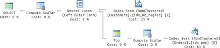
FIGURE 3-2 Plan with a seek per customer.
The critical difference between this plan and the one in Figure 3-1 is that this one applies a seek per customer, not per order. This plan performs 10,000 seeks, costing you 30,000 random reads.
The second step is to query the Orders table to return information about orders whose keys appear in the set of keys returned by the query implementing the first step, like so:
SELECT orderid, orderdate, custid, empid
FROM Sales.Orders
WHERE orderid IN
(SELECT
(SELECT TOP (1) orderid
FROM Sales.Orders AS O
WHERE O.custid = C.custid
ORDER BY orderdate DESC, orderid DESC)
FROM Sales.Customers AS C);
The query plan for the complete solution is shown in Figure 3-3.
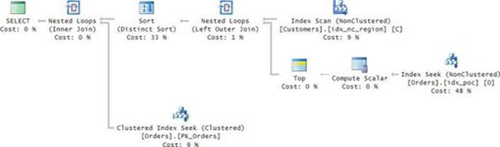
FIGURE 3-3 Complete plan with a seek per customer.
In addition to the work described for the first step of the solution (retrieving the qualifying keys), this plan also performs 10,000 seeks in the index PK_Orders to obtain the desired order attributes for the qualifying orders. That’s after sorting the keys to optimize the seeks. This part adds 10,000 more seeks, giving you a total of 20,000 seeks and resulting in 60,000 random reads. That’s a factor of 500 compared to the previous solution!
When you’re done, run the following code for cleanup:
DROP INDEX idx_poc ON Sales.Orders;
The EXISTS predicate
The EXISTS predicate accepts a subquery as input and returns true or false, depending on whether the subquery returns a nonempty set or an empty one, respectively. As a basic example, the following query returns customers who placed orders:
SELECT custid, companyname
FROM Sales.Customers AS C
WHERE EXISTS (SELECT * FROM Sales.Orders AS O
WHERE O.custid = C.custid);
The predicate is natural to use because it allows you to express requests like the preceding one in SQL in a manner that is similar to the way you express them in a spoken language.
A curious thing about EXISTS is that, unlike most predicates in SQL, it uses two-valued logic. It returns either true or false. It cannot return unknown because there’s no situation where it doesn’t know whether the subquery returns at least one row or none. Pardon the triple-negative form of the last sentence, but for the purposes of this chapter, you want to practice this kind of logic. If the inner query involves a filter, the rows for which the filter predicate evaluates to unknown because of the presence of NULLs are discarded. Still, the EXISTS predicate always knows with certainty whether the result set is empty or not. In contrast to EXISTS, the IN predicate, for example, uses three-valued logic. Consequently, a query using EXISTS can have a different logical meaning than a query using IN when you negate the predicate and NULLs are possible in the data. I’ll demonstrate this later in the chapter.
Another interesting thing about EXISTS is that, from an indexing selection perspective, the optimizer ignores the subquery’s SELECT list. For example, the Orders table has an index called idx_nc_custid defined on the custid column as the key with no included columns. Observe the query plan shown in Figure 3-4 for the last EXISTS query.
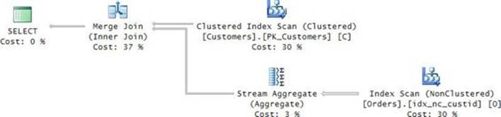
FIGURE 3-4 Plan for EXISTS with SELECT *.
Notice that the only index the plan uses from the Orders table is idx_nc_custid, despite the fact that the subquery uses SELECT *. In other words, this index is considered a covering one for the purposes of this subquery. That’s proof that the SELECT list is ignored for index-selection purposes.
Next I’ll demonstrate a couple of classic tasks that can be handled using the EXISTS predicate. I’ll use a table called T1, which you create and populate by running the following code:
SET NOCOUNT ON;
USE tempdb;
IF OBJECT_ID(N'dbo.T1', N'U') IS NOT NULL DROP TABLE dbo.T1;
CREATE TABLE dbo.T1(col1 INT NOT NULL CONSTRAINT PK_T1 PRIMARY KEY);
INSERT INTO dbo.T1(col1) VALUES(1),(2),(3),(7),(8),(9),(11),(15),(16),(17),(28);
The key column in the table is col1. Suppose you have a key generator that generates consecutive keys starting with 1, but because of deletions you have gaps. One classic challenge is to identify the minimum missing value. To test the correctness of your solution, you can use the small set of sample data that the preceding code generates. For performance purposes, you want to populate the table with a much bigger set. Use the following code to populate it with 10,000,000 rows:
TRUNCATE TABLE dbo.T1;
INSERT INTO dbo.T1 WITH (TABLOCK) (col1)
SELECT n FROM TSQLV3.dbo.GetNums(1, 10000000) AS Nums WHERE n % 10000 <> 0
OPTION(MAXDOP 1);
You can use a CASE expression that returns 1 if 1 doesn’t already exist in the table. The trickier part is identifying the minimum missing value when 1 does exist. One way to achieve this is using the following query:
SELECT MIN(A.col1) + 1 AS missingval
FROM dbo.T1 AS A
WHERE NOT EXISTS
(SELECT *
FROM dbo.T1 AS B
WHERE B.col1 = A.col1 + 1);
The first step in this code is to filter the rows from T1 (aliased as A) where the value in A appears before a missing value. That way, you know the value in A appears before a missing value because you cannot find another value in T1 (aliased as B) where the B value is greater than the A value by 1. Then, from all remaining values in A, you return the minimum plus one. Perhaps you expected the query to finish instantly; after all, there is an index on col1 (PK_T1). Theoretically, you should be able to scan the index in order and short-circuit the work as soon as the first point before a missing value is found. But it takes this query a good few seconds to complete against the large set of sample data. On my system, it took it five seconds to complete. To understand why the query is slow, examine the query plan shown in Figure 3-5.
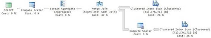
FIGURE 3-5 Plan for a minimum missing value, first attempt.
Observe that the index on col1 is fully scanned twice. The Merge Join operator is used to apply a right anti semi join to detect nonmatches. The Stream Aggregate operator identifies the minimum. The critical thing in this plan that makes it inefficient is that the input is scanned twice fully. There’s no short-circuit even though the scans are ordered.
One attempt to optimize the query is to use the TOP filter instead of the MIN aggregate, like so:
SELECT TOP (1) A.col1 + 1 AS missingval
FROM dbo.T1 AS A
WHERE NOT EXISTS
(SELECT *
FROM dbo.T1 AS B
WHERE B.col1 = A.col1 + 1)
ORDER BY A.col1;
But again, the query is slow. Examine the execution plan of this query, as shown in Figure 3-6.
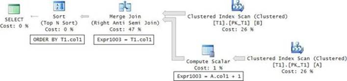
FIGURE 3-6 Plan for a minimum missing value, second attempt.
The Merge Join predicate considers the A input as sorted by Expr1003 (col1 + 1) and the B input by col1 (T1.col1). Because the outer query orders the rows by A.col1 and not by A.col1 + 1, the optimizer doesn’t realize the rows are already sorted and adds a Sort (Top N Sort) operator that consumes the entire input to determine the top 1 row. To fix this, simply change the outer query’s ORDER BY to A.col1 + 1, like so:
SELECT TOP (1) A.col1 + 1 AS missingval
FROM dbo.T1 AS A
WHERE NOT EXISTS
(SELECT *
FROM dbo.T1 AS B
WHERE B.col1 = A.col1 + 1)
ORDER BY A.col1 + 1;
Observe the plan shown in Figure 3-7.
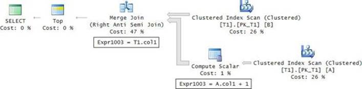
FIGURE 3-7 Plan for a minimum missing value, third attempt.
Now the optimizer realizes that the Merge Join operator returns the rows sorted the same way the TOP filter needs them, so it can short-circuit as soon as the first matching row is found. The query finishes in sub-second time.
Alternatively, you will also get an optimal plan if you change the inner query’s WHERE filter from B.col1 = A.col1 + 1 to A.col1 = B.col1 – 1, and the ORDER BY clause from A.col1 + 1 to A.col1, like so:
SELECT TOP (1) A.col1 + 1 AS missingval
FROM dbo.T1 AS A
WHERE NOT EXISTS
(SELECT *
FROM dbo.T1 AS B
WHERE A.col1 = B.col1 - 1)
ORDER BY A.col1;
Now add the logic with the CASE expression to return 1 when 1 doesn’t exist and to return the result of the subquery (using one of the efficient solutions) otherwise. You get the following complete solution:
SELECT
CASE
WHEN NOT EXISTS(SELECT * FROM dbo.T1 WHERE col1 = 1) THEN 1
ELSE (SELECT TOP (1) A.col1 + 1 AS missingval
FROM dbo.T1 AS A
WHERE NOT EXISTS
(SELECT *
FROM dbo.T1 AS B
WHERE B.col1 = A.col1 + 1)
ORDER BY missingval)
END AS missingval;
Another classic task involving a sequence of values is to identify all ranges of missing values. In our case, we’ll look for the ones missing between the minimum and maximum that exist in the table. This task is generally known as identifying gaps. Here, unlike with the minimum missing-value task, there’s no potential for a short circuit. As the first step, you can use the same query you used in the previous task to find all values that appear before a gap:
SELECT col1
FROM dbo.T1 AS A
WHERE NOT EXISTS
(SELECT *
FROM dbo.T1 AS B
WHERE B.col1 = A.col1 + 1);
You get the following output against the small set of sample data:
col1
-----------
3
9
11
17
28
Observe that you also get the maximum value in the table (28) because that value plus 1 doesn’t exist. But this value doesn’t represent a gap you want to return. To exclude it from the output, add the following predicate to the outer query’s filter:
AND col1 < (SELECT MAX(col1) FROM dbo.T1)
Now that you are left with only values that appear before gaps, you need to identify for each current value the related value that appears right after the gap. You can do this in the outer query’s SELECT list with the following subquery, which returns for each current value the minimum value that is greater than the current one:
(SELECT MIN(B.col1)
FROM dbo.T1 AS B
WHERE B.col1 > A.col1)
You might think it’s a bit strange to use the alias B both here and in the subquery that checks that the value plus 1 doesn’t exist. However, because the two subqueries have independent scopes, there’s no problem with that.
Last, you add one to the value before the gap and subtract one from the value after the gap to get the actual gap information. Putting it all together, here’s the complete solution:
SELECT col1 + 1 AS range_from,
(SELECT MIN(B.col1)
FROM dbo.T1 AS B
WHERE B.col1 > A.col1) - 1 AS range_to
FROM dbo.T1 AS A
WHERE NOT EXISTS
(SELECT *
FROM dbo.T1 AS B
WHERE B.col1 = A.col1 + 1)
AND col1 < (SELECT MAX(col1) FROM dbo.T1);
This query generates the following output:
range_from range_to
----------- -----------
4 6
10 10
12 14
18 27
The execution plan for this solution is shown in Figure 3-8.
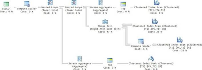
FIGURE 3-8 Plan for the gaps query.
The plan is quite efficient, especially when there’s a small number of gaps. The three rightmost operators in the upper branch handle the computation of the maximum col1 value in the table. The value is obtained from the tail of the index, so the work is negligible. The middle section uses a Merge Join (Right Anti Semi Join) operator to identify the values that appear before gaps. The merge algorithm relies on two ordered scans of the index on col1. This strategy is much more efficient than the alternative, which is to apply an index seek per original value in the sequence. Finally, the bottom branch applies an index seek per filtered value (a value that appears before a gap) to identify the respective value after the gap. What’s important here is that you get an index seek per filtered value (namely, per gap) and not per original value. So, especially when the number of gaps is small, you get a small number of seeks. For example, the large set of sample data has 10,000,000 rows with 1,000 gaps. With this sample data, the query finishes in five seconds on my system. Chapter 4, “Grouping, pivoting, and windowing,” continues the discussion about identifying gaps and shows additional solutions.
When you’re done, run the following code for cleanup:
IF OBJECT_ID(N'dbo.T1', N'U') IS NOT NULL DROP TABLE dbo.T1;
One of the interesting things about T-SQL querying tasks is that, for any given problem, there are usually many possible solutions. Often, different solutions get different execution plans. So it’s important to develop the skill of solving querying tasks in different ways and observing carefully in each case how the optimizer handles things. Later, when you tune a query and need to achieve a certain effect on the plan, it’s easier if you already know which change is likely to give you such an effect—for example, by comparing how SQL Server handles a solution based on a subquery versus one that uses a join, how it handles a solution using an aggregate versus one that uses the TOP filter, and so on. Another example for different approaches is applying positive logic versus negative logic. For instance, recall from the beginning of the chapter the task to identify customers for whom all employees handled orders. The solution I presented for the task applied positive logic:
USE TSQLV3;
SELECT custid
FROM Sales.Orders
GROUP BY custid
HAVING COUNT(DISTINCT empid) = (SELECT COUNT(*) FROM HR.Employees);
Another approach is to apply negative logic, but because what you’re after is positive—customers for whom all employees handled orders—you will need two negations to get the same meaning. It’s just like saying that something is common is the same as saying that it is not uncommon. In our case, saying customers for whom all employees handled orders is like saying customers for whom no employees handled no orders. This translates to the following query with two NOT EXISTS predicates, one nested inside the other:
SELECT custid, companyname
FROM Sales.Customers AS C
WHERE NOT EXISTS
(SELECT * FROM HR.Employees AS E
WHERE NOT EXISTS
(SELECT * FROM Sales.Orders AS O
WHERE O.custid = C.custid
AND O.empid = E.empid));
Perhaps the double-negative form is not very intuitive initially, but the good news is that this kind of thinking can improve with practice.
Now you can examine and compare the plans for the positive solutions versus the negative solutions to learn how the optimizer handles things in the different cases. Note, though, that the tables in the TSQLV3 database are very small, so you can’t really do any performance testing with them. You will need much bigger tables to do proper performance analysis and tuning. I demonstrate an example with bigger volumes of data where the double-negative approach enables a very efficient solution in the article “Identifying a Subsequence in a Sequence, Part 2,” which you can find here: http://sqlmag.com/t-sql/identifying-subsequence-in-sequence-part-2.
I found the double-negative approach to be handy in a number of other cases. For example, suppose you have a character string column called sn (for serial number) that is supposed to allow only digits. You want to enforce this rule with a CHECK constraint. You can phrase a predicate that is based on positive logic, but I find the double-negative form to be the most elegant and economic in this case. The positive rule says that every character in the column is a digit. The double-negative form is that no character in the column is not a digit. In T-SQL, this rule translates to the following predicate:
sn NOT LIKE '%[^0-9]%'
Nice and simple!
Misbehaving subqueries
There are common tasks that are handled with subqueries for which you can easily get into trouble with bugs when you don’t follow certain best practices. I’ll describe two such problems: one involving a substitution error in a subquery column name, and another involving unintuitive handling of NULLs in a subquery. I’ll also provide best practices that, if followed, can help you avoid getting into such trouble.
Consider the following T1 and T2 tables and the sample data they are populated with:
IF OBJECT_ID(N'dbo.T1', N'U') IS NOT NULL DROP TABLE dbo.T1;
IF OBJECT_ID(N'dbo.T2', N'U') IS NOT NULL DROP TABLE dbo.T2;
GO
CREATE TABLE dbo.T1(col1 INT NOT NULL);
CREATE TABLE dbo.T2(col2 INT NOT NULL);
INSERT INTO dbo.T1(col1) VALUES(1);
INSERT INTO dbo.T1(col1) VALUES(2);
INSERT INTO dbo.T1(col1) VALUES(3);
INSERT INTO dbo.T2(col2) VALUES(2);
Suppose you need to return the values in T1 that also appear in the set of values in T2. You write the following query (but don’t run it yet).
SELECT col1 FROM dbo.T1 WHERE col1 IN(SELECT col1 FROM dbo.T2);
Before you execute this query, examine the values in both tables and answer the question, which values do you expect to see in the result? Naturally, you expect to see only the value 2 in the result. Now execute the query. You get the following output:
col1
-----------
1
2
3
Can you explain why you’re getting all values from T1 and not just 2?
A close examination of the table definitions and the query code will reveal that the subquery against T2 refers to col1 by mistake, instead of col2. Now the question is, why didn’t the code fail? The way SQL resolves which table the column belongs to is it first looks for the column in the table in the immediate query. If it cannot find it there, like in our case, it looks for it in the table in the outer query. In our case, there is a column named col1 in the outer table; therefore, that one is used. Unintentionally, the inner reference to col1 became a correlated reference. So when the outer col1 value is 1, the inner query selects a 1 for every row in T2. When the outer col1 value is 2, the inner query selects a 2 for every row in T2. You realize that as long as there are rows in T2, and the col1 value is not NULL, you’ll always get a match.
Usually, this type of problem happens when you are not consistent in naming attributes the same way in different tables when they represent the same thing. For example, suppose that in a Customers table you name the column holding the customer ID custid, and in a related Orders table you name the column customerid. Then you write a query similar to the query in our example looking for customers who placed orders, but by mistake you specify custid against both tables. You will get all customers back instead of just the ones who truly placed orders. When the outer statement is SELECT, the query returns an incorrect result with all rows, but you realize that when the outer statement is DELETE, you end up deleting all rows.
There are two best practices that can help you avoid such bugs in your code: one is a long-term recommendation, and the other is a short-term one. The long-term best practice is to pay more attention to naming attributes in different tables the same way when they represent the same thing. The short-term recommendation is to simply prefix the column name with the table name (or alias, if you assigned one), and then you’re not allowing implied resolution. Apply this practice to our sample query:
SELECT col1 FROM dbo.T1 WHERE col1 IN(SELECT T2.col1 FROM dbo.T2);
Now the query fails with a resolution error saying there’s no column called col1 in T2:
Msg 207, Level 16, State 1, Line 278
Invalid column name 'col1'.
Seeing this error, you will of course figure out the problem and fix the query by specifying the right column name, col2, in the subquery.
Another classic case where people get into trouble with subqueries has to do with the complexities that are related to the NULL treatment. To see the problem, re-create and repopulate the T1 and T2 tables with the following code:
IF OBJECT_ID(N'dbo.T1', N'U') IS NOT NULL DROP TABLE dbo.T1;
IF OBJECT_ID(N'dbo.T2', N'U') IS NOT NULL DROP TABLE dbo.T2;
GO
CREATE TABLE dbo.T1(col1 INT NULL);
CREATE TABLE dbo.T2(col1 INT NOT NULL);
INSERT INTO dbo.T1(col1) VALUES(1);
INSERT INTO dbo.T1(col1) VALUES(2);
INSERT INTO dbo.T1(col1) VALUES(NULL);
INSERT INTO dbo.T2(col1) VALUES(2);
INSERT INTO dbo.T2(col1) VALUES(3);
Observe the values in both tables. Suppose you want to return only the values that appear in T2 but not in T1. You write the following code in an attempt to achieve this (but don’t run it yet):
SELECT col1 FROM dbo.T2 WHERE col1 NOT IN(SELECT col1 FROM dbo.T1);
Before you run the code, answer the question, which values do you expect to see in the result? Most people expect to get the value 3 back. Now run the query. You get an empty set back:
col1
-----------
A key to understanding why you get an empty set is remembering that for a WHERE filter to return a row, the predicate needs to evaluate to true; getting false or unknown causes the row to be discarded. It’s clear why you don’t get the value 2 back—because the value 2 does appear in T1 (the IN predicate returns true), you don’t want to see it (the NOT IN is false). The trickier part is to figure out why you don’t get the value 3 back. The answer to the question whether 3 appears in T1 is unknown because the NULL can represent any value. More technically, the IN predicate translates to 3=1 OR 3=2 OR 3=NULL, and the result of this disjunction of predicates is the logical value unknown. Now apply NOT to the result. When you negate unknown, you still get unknown. In other words, just like it’s unknown that 3 appears in T1, it’s also unknown that 3 doesn’t appear in T1.
All this means is that when you use NOT IN with a subquery and at least one of the members of the subquery’s result is NULL, the query will return an empty set. From a SQL perspective, you don’t want to see the values from T2 that appear in T1 exactly, because you know with certainty that they appear in T1, and you don’t want to see the rest of the values from T2, because you don’t know with certainty that they don’t appear in T1. This is one of the absurd implications of NULL handling and the three-valued logic.
You can do certain things to avoid getting into such trouble. For one, if a column is not supposed to allow NULLs, make sure you enforce a NOT NULL constraint. If you don’t, chances are that NULLs will find their way into that column. For another, if the column is indeed supposed to allow NULLs, but for example those NULLs represent a missing and inapplicable value, you need to revise your solution to ignore them. You can achieve this behavior in a couple of ways. One option is to explicitly remove the NULLs in the inner query by adding the filter WHERE col1 IS NOT NULL, like so:
SELECT col1 FROM dbo.T2 WHERE col1 NOT IN(SELECT col1 FROM dbo.T1 WHERE col1 IS NOT NULL);
This time, you get the result you probably expected to begin with:
col1
-----------
3
The other option is to use NOT EXISTS instead of NOT IN, like so:
SELECT col1
FROM dbo.T2
WHERE NOT EXISTS(SELECT * FROM dbo.T1 WHERE T1.col1 = T2.col1);
Here, when the inner query’s filter compares a NULL with anything, the result of the filter predicate is unknown, and rows for which the predicate evaluates to unknown are discarded. In other words, the implicit removal of the NULLs by the filter in this solution has the same effect as the explicit removal of the NULLs in the previous solution.
Table expressions
Table expressions are named queries you interact with similar to the way you interact with tables. T-SQL supports four kinds of table expressions: derived tables, common table expressions (CTEs), views, and inline table-valued functions (inline TVFs). The first two are visible only in the scope of the statement that defines them. With the last two, the definition of the table expression is stored as a permanent object in the database, and anyone with the right permissions can interact with them.
A query against a table expression involves three parts in the code: the inner query, the name that you assign to the table expression (and when relevant, its columns), and the outer query. The inner query is supposed to generate a table result. This means it needs to satisfy three requirements:
![]() The inner query cannot have a presentation ORDER BY clause. It can have an ORDER BY clause to support a TOP or OFFSET-FETCH filter, but then the outer query doesn’t give you assurance that the rows will be presented in any particular order, unless it has its own ORDER BY clause.
The inner query cannot have a presentation ORDER BY clause. It can have an ORDER BY clause to support a TOP or OFFSET-FETCH filter, but then the outer query doesn’t give you assurance that the rows will be presented in any particular order, unless it has its own ORDER BY clause.
![]() All columns must have names. So, if you have a column that results from a computation, you must assign it with a name using an alias.
All columns must have names. So, if you have a column that results from a computation, you must assign it with a name using an alias.
![]() All column names must be unique. So, if you join tables that have columns with the same name and you need to return the columns with the same name, you’ll need to assign them with different aliases. Table names or aliases that are used as prefixes for the column names in intermediate logical-processing phases are removed when a table expression is defined based on the query. Therefore, the column names in the table expression have to be unique as standalone, unqualified, ones.
All column names must be unique. So, if you join tables that have columns with the same name and you need to return the columns with the same name, you’ll need to assign them with different aliases. Table names or aliases that are used as prefixes for the column names in intermediate logical-processing phases are removed when a table expression is defined based on the query. Therefore, the column names in the table expression have to be unique as standalone, unqualified, ones.
As long as a query satisfies these three requirements, it can be used as the inner query in a table expression.
From a physical processing perspective, the inner query’s result doesn’t get persisted anywhere; rather, it is inlined. This means that the outer query and the inner query are merged. When you look at a plan for a query against a table expression, you see the plan interacting with the underlying physical structures directly after the query got inlined. In other words, there’s no physical side to table expressions; rather, they are virtual and should be considered to be a logical tool. The one exception to this rule is when using indexed views—in which case, the view result gets persisted in a B-tree. For details see http://msdn.microsoft.com/en-us/library/ms191432.aspx).
The following sections describe the different kinds of table expressions.
Derived tables
A derived table is probably the type of table expression that most closely resembles a subquery. It is a table subquery that is defined in the FROM clause of the outer query. You use the following form to define and query a derived table:
SELECT <col_list> FROM (<inner_query>) AS <table_alias>[(<target_col_list>)];
Remember that all columns of a table expression must have names; therefore, you have to assign column aliases to all columns that are results of computations. Derived tables support two different syntaxes for assigning column aliases: inline aliasing and external aliasing. To demonstrate the syntaxes, I’ll use a table called T1 that you create and populate by running the following code:
IF OBJECT_ID(N'dbo.T1', N'U') IS NOT NULL DROP TABLE dbo.T1;
GO
CREATE TABLE dbo.T1(col1 INT);
INSERT INTO dbo.T1(col1) VALUES(1);
INSERT INTO dbo.T1(col1) VALUES(2);
Suppose you need the inner query to define a column alias called expr1 for the computation col1 + 1, and then in the outer query refer to expr1 in one of the expressions. Using the inline aliasing form, you specify the computation followed by the AS clause followed by the alias, like so:
SELECT col1, exp1 + 1 AS exp2
FROM (SELECT col1, col1 + 1 AS exp1
FROM dbo.T1) AS D;
Using the external aliasing form, you specify the target column aliases in parentheses right after the derived table name, like so:
SELECT col1, exp1 + 1 AS exp2
FROM (SELECT col1, col1 + 1
FROM dbo.T1) AS D(col1, exp1);
With this syntax, you have to specify names for all columns, even the ones that already have names.
Both syntaxes are standard. Each has its own advantages. What I like about the inline aliasing form is that with long and complex queries it’s easy to identify which alias represents which computation. What I like about the external form is that it’s easy to see in one place which columns the table expression contains. You need to make a decision about which syntax is more convenient for you to use. If you want, you can combine both, like so:
SELECT col1, exp1 + 1 AS exp2
FROM (SELECT col1, col1 + 1 AS exp1
FROM dbo.T1) AS D(col1, exp1);
In case of a conflict, the alias assigned externally is used.
From a language-design perspective, derived tables have two weaknesses. One has to do with nesting and the other with multiple references. Both are results of the derived table being defined in the FROM clause of the outer query. Regarding nesting: if you need to make references from one derived table to another, you need to nest those tables. The problem with nesting is that it can make it hard to follow the logic when you need to review or troubleshoot the code. As an example, consider the following query where derived tables are used to enable the reuse of column aliases:
SELECT orderyear, numcusts
FROM (SELECT orderyear, COUNT(DISTINCT custid) AS numcusts
FROM (SELECT YEAR(orderdate) AS orderyear, custid
FROM Sales.Orders) AS D1
GROUP BY orderyear) AS D2
WHERE numcusts > 70;
The query returns order years and the distinct number of customers handled in each year for years that had more than 70 distinct customers handled.
Trying to figure out what the code does by reading it from top to bottom is tricky because the outer query is interrupted in the middle by the derived table D2, and then the query defining D2 is interrupted in the middle by the derived table D1. Human brains are not very good at analyzing nested units; they are better at analyzing independent modules where you focus your attention on one unit at a time, from start to end, in an uninterrupted way. So, typically what you do to try and make sense out of such nested code is analyze it from the innermost derived table (D1, in this example), and then gradually work outward, rather than analyzing it in a more natural order.
As for physical processing, as mentioned, table expressions don’t get persisted anywhere; instead, they get inlined. This can be seen clearly in the execution plan of the query, as shown in Figure 3-9.

FIGURE 3-9 Table expressions that are inlined.
There are no spool operators representing work tables; rather, the plan interacts with the Orders table directly.
In addition to the nesting aspect, another weakness of derived tables relates to cases where you need multiple references to the same table expression. Take the following query as an example:
SELECT CUR.orderyear, CUR.numorders, CUR.numorders - PRV.numorders AS diff
FROM (SELECT YEAR(orderdate) AS orderyear, COUNT(*) AS numorders
FROM Sales.Orders
GROUP BY YEAR(orderdate)) AS CUR
LEFT OUTER JOIN
(SELECT YEAR(orderdate) AS orderyear, COUNT(*) AS numorders
FROM Sales.Orders
GROUP BY YEAR(orderdate)) AS PRV
ON CUR.orderyear = PRV.orderyear + 1;
The query computes the number of orders that were handled in each year, and the difference from the count of the previous year. There are actually simpler and more efficient ways to handle this task—for example, with the LEAD function—but this code is used for illustration purposes. Observe that the outer query joins two derived tables that are based on the exact same query that computes the yearly order counts. SQL doesn’t allow you to define and name a derived table once and then refer to it multiple times in the same FROM clause that defines it. Unfortunately, you have to repeat the code. This makes the code longer and harder to maintain. Every time you need to make a change in the derived table query, you need to remember to make it in all copies, which increases the likelihood of errors.
CTEs
Common table expressions (CTEs) are another kind of table expression that, like derived tables, are visible only to the statement that defines them. There are no session-scoped or batch-scoped CTEs. The nice thing about CTEs is that they were designed to resolve the two weaknesses that derived tables have. Here’s an example of a CTE definition representing yearly order counts:
WITH OrdCount
AS
(
SELECT
YEAR(orderdate) AS orderyear,
COUNT(*) AS numorders
FROM Sales.Orders
GROUP BY YEAR(orderdate)
)
SELECT orderyear, numorders
FROM OrdCount;
You will find here the same components you have in code interacting with a derived table—namely, there’s the CTE name, the inner query, and the outer query. The difference between CTEs and derived tables is in how these three components are arranged with respect to each another. Observe that the code starts with naming the CTE, continues with the inner query expressed from start to end uninterrupted, and then the outer query also is expressed from start to end uninterrupted. This design makes CTEs easier to work with than derived tables.
Recall the example with the nesting of derived tables. Here’s the alternative using CTEs:
WITH C1 AS
(
SELECT YEAR(orderdate) AS orderyear, custid
FROM Sales.Orders
),
C2 AS
(
SELECT orderyear, COUNT(DISTINCT custid) AS numcusts
FROM C1
GROUP BY orderyear
)
SELECT orderyear, numcusts
FROM C2
WHERE numcusts > 70;
As you can see, in the same WITH statement you can define multiple CTEs separated by commas. Each can refer in the inner query to all previously defined CTEs. Then the outer query can refer to all CTEs defined by that WITH statement. The nice thing about this approach is that the units are not nested; rather, they are expressed one at a time in an uninterrupted manner. So, if you need to figure out the logic of the code, you analyze it in a more natural order from top to bottom.
The one thing I find a bit tricky when troubleshooting a WITH statement with multiple CTEs is that, if you want to check the result of an intermediate CTE, you cannot just highlight the code down to that part and run it. You need to inject a SELECT * FROM <ctename> right after that CTE and then run the code down to that part. Derived tables have an advantage in this respect in the sense that, without any code changes, you can highlight a query against a derived table including all the units you want to test and run it.
From a physical-processing perspective, the treatment of CTEs is the same as that for derived tables. The results of the inner queries don’t get persisted anywhere; rather, the code gets inlined. This code generates the same plan as the one shown earlier for derived tables in Figure 3-9.
The other advantage of using CTEs rather than derived tables is that, because you name the CTE before using it, you are allowed to refer to the CTE name multiple times in the outer query without needing to repeat the code. Recall the example shown earlier with two copies of the same derived table to return yearly counts of orders and the difference from the previous yearly count. Here’s the CTE-based alternative:
WITH OrdCount
AS
(
SELECT
YEAR(orderdate) AS orderyear,
COUNT(*) AS numorders
FROM Sales.Orders
GROUP BY YEAR(orderdate)
)
SELECT CUR.orderyear, CUR.numorders,
CUR.numorders - PRV.numorders AS diff
FROM OrdCount AS CUR
LEFT OUTER JOIN OrdCount AS PRV
ON CUR.orderyear = PRV.orderyear + 1;
Clearly, this is a better design.
Note that because SQL Server doesn’t persist the table expression’s result anywhere, whether you use derived tables or CTEs, all references to the table expression’s name will be expanded, and the work will be repeated. This can be seen clearly in the plan shown in Figure 3-10.
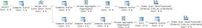
FIGURE 3-10 Work that is repeated with multiple references.
You can see the work happening twice. A covering index from the Orders table is scanned twice, and then the rows are sorted, grouped, and aggregated twice. If the table is large and you want to avoid repeating all this work, you should consider using a temporary table or a table variable instead.
Recursive CTEs
T-SQL supports a specialized form of a CTE with recursive syntax. To describe and demonstrate recursive CTEs, I’ll use a table called Employees that you create and populate by running the following code:
SET NOCOUNT ON;
USE tempdb;
IF OBJECT_ID(N'dbo.Employees', N'U') IS NOT NULL DROP TABLE dbo.Employees;
CREATE TABLE dbo.Employees
(
empid INT NOT NULL
CONSTRAINT PK_Employees PRIMARY KEY,
mgrid INT NULL
CONSTRAINT FK_Employees_Employees FOREIGN KEY REFERENCES dbo.Employees(empid),
empname VARCHAR(25) NOT NULL,
salary MONEY NOT NULL
);
INSERT INTO dbo.Employees(empid, mgrid, empname, salary)
VALUES(1, NULL, 'David' , $10000.00),
(2, 1, 'Eitan' , $7000.00),
(3, 1, 'Ina' , $7500.00),
(4, 2, 'Seraph' , $5000.00),
(5, 2, 'Jiru' , $5500.00),
(6, 2, 'Steve' , $4500.00),
(7, 3, 'Aaron' , $5000.00),
(8, 5, 'Lilach' , $3500.00),
(9, 7, 'Rita' , $3000.00),
(10, 5, 'Sean' , $3000.00),
(11, 7, 'Gabriel', $3000.00),
(12, 9, 'Emilia' , $2000.00),
(13, 9, 'Michael', $2000.00),
(14, 9, 'Didi' , $1500.00);
CREATE UNIQUE INDEX idx_nc_mgr_emp_i_name_sal
ON dbo.Employees(mgrid, empid) INCLUDE(empname, salary);
Recursive CTEs have a body with not just one member like regular CTEs, but rather multiple members. Usually, you will have one anchor member and one recursive member, but the syntax certainly allows having multiple anchor members and multiple recursive members. I’ll explain the roles of the members through an example. The following code returns all direct and indirect subordinates of employee 3:
WITH EmpsCTE AS
(
SELECT empid, mgrid, empname, salary
FROM dbo.Employees
WHERE empid = 3
UNION ALL
SELECT C.empid, C.mgrid, C.empname, C.salary
FROM EmpsCTE AS P
JOIN dbo.Employees AS C
ON C.mgrid = P.empid
)
SELECT empid, mgrid, empname, salary
FROM EmpsCTE;
The first query you see in the CTE body is the anchor member. The anchor member is a regular query that can run as a self-contained one and executes only once. This query creates the initial result set that is then used by the recursive member. In our case, the anchor query returns the row for employee 3. Then, in the CTE body, the code uses a UNION ALL operator to indicate that the result of the anchor query should be unified with the results of the recursive query that comes next. The recursive member executes repeatedly until it returns an empty set. What makes it recursive is the reference that it has to the CTE name. This reference represents the immediate previous result set. In our case, the recursive query joins the immediate previous result set holding the managers from the previous round with the Employees table to obtain the direct subordinates of those managers. As soon as the recursive query cannot find another level of subordinates, it stops executing. Then the reference to the CTE name in the outer query represents the unified result sets of the anchor and recursive members. Here’s the output generated by this code:
empid mgrid empname salary
------ ------ -------- --------
3 1 Ina 7500.00
7 3 Aaron 5000.00
9 7 Rita 3000.00
11 7 Gabriel 3000.00
12 9 Emilia 2000.00
13 9 Michael 2000.00
14 9 Didi 1500.00
The execution plan for this query is shown in Figure 3-11.
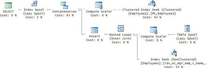
FIGURE 3-11 Plan for a recursive query.
The plan creates a B-tree-based worktable (Index Spool operator) where it stores the intermediate result sets. The plan performs a seek in the clustered index to retrieve the row for employee 3 and writes it to the spool. The plan then repeatedly reads the last round’s result from the spool, joining it with the covering index from the Employees table to retrieve the employees from the next level, and it writes those to the spool. The plan keeps a count of how many times the recursive member was executed. It does so by using two Compute Scalar operators. The first initializes a variable with 0, and the second increments the variable by 1 in each iteration. Then the Assert operator fails the query if the counter is greater than 100. In other words, by default the recursive member is allowed to run up to 100 times. You can change the default to the limit you want to set using a query option called MAXRECURSION. To remove the limit, set it to 0. You specify the option in an OPTION clause at the end of the outer query—for example, OPTION(MAXRECURSION 10).
The main benefits I see in recursive queries are the brevity of the code and the ability to traverse graph structures based only on the parent and child IDs (mgrid and empid, in our example). The main drawback of recursive queries is performance. They tend to perform less efficiently than alternative methods, even your own loop-based solutions. With recursive queries, you don’t have any control over the worktable; for example, you can’t define your own indexes on it, you can’t define how to filter the rows from the previous round, and so on. If you know how to optimize T-SQL code, you can usually get better performance with your own solution.
For more information about recursive queries and handling graph structures, see Chapter 11, “Graphs and recursive queries.”
Views
Derived tables and CTEs are available only to the statement that defines them. Once the defining statement finishes, they are gone. If you need the ability to reuse the table expression beyond the single statement, you can use views or inline TVFs. Views and inline TVFs are stored as an object in the database and therefore are reusable by users with the right permissions. What gets stored in the database is the query definition and metadata information, not the data (with the exception of an indexed view as mentioned earlier). When submitting a query or a modification against the table expression, SQL Server inlines the table expression and applies the query or modification to the underlying object.
As an example, suppose you have different branches in your organization. You want users from the USA branch to be able to interact only with customers from the USA. SQL Server doesn’t have built-in support for row-level permissions. So you create the following view querying the Customers table and filtering only customers from the USA:
USE TSQLV3;
IF OBJECT_ID(N'Sales.USACusts', N'V') IS NOT NULL DROP VIEW Sales.USACusts;
GO
CREATE VIEW Sales.USACusts WITH SCHEMABINDING
AS
SELECT
custid, companyname, contactname, contacttitle, address,
city, region, postalcode, country, phone, fax
FROM Sales.Customers
WHERE country = N'USA'
WITH CHECK OPTION;
You grant the users from the USA permissions against the view but not against the underlying table.
The SCHEMABINDING option ensures that structural changes against referenced objects and columns will be rejected. This option requires schema-qualifying object names and explicit enumeration of the column list (no *). The CHECK OPTION ensures that modifications against the view that contradict the inner query’s filter are rejected. For example, with this option you won’t be allowed to insert a customer from the UK through the view. You also won’t be allowed to update the country/region to one other than the USA through the view.
Now when you query the view, you interact only with customers from the USA, like in the following example:
SELECT custid, companyname
FROM Sales.USACusts
ORDER BY region, city;
As mentioned, behind the scenes SQL Server will inline the inner query, so the execution plan you get will be the same as the one you will get for this query:
SELECT custid, companyname
FROM Sales.Customers
WHERE country = N'USA'
ORDER BY region, city;
Note that despite the fact that the view’s inner query gets inlined, sometimes SQL Server cannot avoid doing work even when, intuitively, you think it should. Consider an example where you perform vertical partitioning of a wide table, storing in each narrower table the key and a different subset of the original columns. Then you use a view to join the tables to make it look like one relation. Use the following code to create a basic example for such an arrangement:
IF OBJECT_ID(N'dbo.V', N'V') IS NOT NULL DROP VIEW dbo.V;
IF OBJECT_ID(N'dbo.T3', N'U') IS NOT NULL DROP TABLE dbo.T3;
IF OBJECT_ID(N'dbo.T2', N'U') IS NOT NULL DROP TABLE dbo.T2;
IF OBJECT_ID(N'dbo.T1', N'U') IS NOT NULL DROP TABLE dbo.T1;
GO
CREATE TABLE dbo.T1
(
keycol INT NOT NULL CONSTRAINT PK_T1 PRIMARY KEY,
col1 INT NOT NULL
);
CREATE TABLE dbo.T2
(
keycol INT NOT NULL
CONSTRAINT PK_T2 PRIMARY KEY
CONSTRAINT FK_T2_T1 REFERENCES dbo.T1,
col2 INT NOT NULL
);
CREATE TABLE dbo.T3
(
keycol INT NOT NULL
CONSTRAINT PK_T3 PRIMARY KEY
CONSTRAINT FK_T3_T1 REFERENCES dbo.T1,
col3 INT NOT NULL
);
GO
CREATE VIEW dbo.V WITH SCHEMABINDING
AS
SELECT T1.keycol, T1.col1, T2.col2, T3.col3
FROM dbo.T1
INNER JOIN dbo.T2
ON T1.keycol = T2.keycol
INNER JOIN dbo.T3
ON T1.keycol = T3.keycol;
GO
Note that I’m not getting into a discussion here about whether this is a good design or a bad one—I’m just trying to explain how optimization of code against table expressions works. Suppose you know there’s a one-to-one relationship between all tables. Every row in one table has exactly one matching row in each of the other tables. You issue a query against the view requesting columns that originate in only one of the tables:
SELECT keycol, col1 FROM dbo.V;
Some people intuitively expect the optimizer to be smart enough to know that only T1 should be accessed. The problem is that SQL Server doesn’t know what you know—that there’s a one-to-one relationship between the tables. As far as SQL Server is concerned, there could be rows in T1 that don’t have related rows in the other tables and therefore shouldn’t be returned. Also, there could be rows in T1 that have multiple related rows in the other tables and therefore should be returned multiple times. In other words, the optimizer has to create a plan where it joins T1 with T2 and T3 as shown in Figure 3-12.
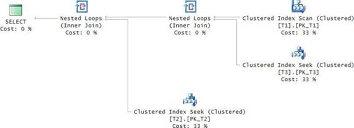
FIGURE 3-12 Plan that shows access to all tables.
To access only T1 to get what you want, you have to query T1 directly and not through the view. I’m using this example to emphasize that sometimes issuing a query through a view (or any other type of table expression) will involve more work than querying only what you think the relevant underlying objects are. That’s despite the fact that the inner query gets inlined.
A quick puzzle
Query only col2 from the view and, before looking at the plan, try to guess which tables should be accessed. Then examine the plan and try to explain what you see. Perhaps you expected all three tables to be accessed based on the previous example, but you will find that T2 and T3 are accessed but not T1. The optimizer realizes that, thanks to the existing foreign-key relationships, every row in T2 and T3 has exactly one matching row in T1. The other way around is not necessarily true; theoretically, a row in T1 can have zero, one, or more matching rows in T2 and T3. Also, inner joins are commutative, meaning that (T1 JOIN T2) JOIN T3 is equivalent to T1 JOIN (T2 JOIN T3). So when asking only for a column from T2, it’s enough to join T2 with T3 to get the correct result. The join to T1 becomes redundant. It’s nice to see that the optimizer is capable of such tricks. But you do still pay for the join to T3 because, theoretically, this join can affect the result. As mentioned, if you want the optimal plan, you need to access the underlying table directly and not through the view. The same optimization considerations apply to all types of table expressions, not just views.
When you’re done, run the following code for cleanup:
IF OBJECT_ID(N'dbo.V', N'V') IS NOT NULL DROP VIEW dbo.V;
IF OBJECT_ID(N'dbo.T3', N'U') IS NOT NULL DROP TABLE dbo.T3;
IF OBJECT_ID(N'dbo.T2', N'U') IS NOT NULL DROP TABLE dbo.T2;
IF OBJECT_ID(N'dbo.T1', N'U') IS NOT NULL DROP TABLE dbo.T1;
Inline table-valued functions
Suppose you need a reusable table expression like a view, but you also need to be able to pass input parameters to the table expression. Views do not support input parameters. For this purpose, SQL Server provides you with inline table-valued functions (TVFs). As an example, the following code creates an inline TVF called GetTopOrders that accepts as inputs a customer ID and a number and returns the requested number of most-recent orders for the input customer:
IF OBJECT_ID(N'dbo.GetTopOrders', N'IF') IS NOT NULL DROP FUNCTION dbo.GetTopOrders;
GO
CREATE FUNCTION dbo.GetTopOrders(@custid AS INT, @n AS BIGINT) RETURNS TABLE
AS
RETURN
SELECT TOP (@n) orderid, orderdate, empid
FROM Sales.Orders
WHERE custid = @custid
ORDER BY orderdate DESC, orderid DESC;
GO
The following code queries the function to return the three most recent orders for customer 1:
SELECT orderid, orderdate, empid
FROM dbo.GetTopOrders(1, 3) AS O;
SQL Server inlines the inner query and performs parameter embedding, meaning that it replaces the parameters with constants. After inlining and embedding, the query that actually gets optimized is the following:
SELECT TOP (3) orderid, orderdate, empid
FROM Sales.Orders
WHERE custid = 1
ORDER BY orderdate DESC, orderid DESC;
I find inline TVFs to be a great tool, allowing for the encapsulation of the logic and reusability without any performance penalties. I’m afraid I cannot say the same thing about the other types of user-defined functions (UDFs). I elaborate on performance problems of UDFs in Chapter 9, “Programmable objects.”
Generating numbers
One of my favorite tools in T-SQL, if not the favorite, is a function that returns a sequence of integers in a requested range. Such a function has so many practical uses that I’m surprised SQL Server doesn’t provide it as a built-in tool. Fortunately, by employing a few magical tricks, you can create a very efficient version of such a function yourself as an inline TVF.
Before looking at my version, I urge you to try and come up with yours. It’s a great challenge. Create a function called GetNums that accepts the inputs @low and @high and returns a sequence of integers in the requested range. The goal is best-possible performance. You will use the function to generate millions of rows in some cases, so naturally you will want it to perform well.
There are three critical things I rely on to get a performant solution:
![]() Generating a large number of rows with cross joins
Generating a large number of rows with cross joins
![]() Generating row numbers efficiently without sorting
Generating row numbers efficiently without sorting
![]() Short-circuiting the work with TOP when the requested number of rows is reached
Short-circuiting the work with TOP when the requested number of rows is reached
The first step is to generate a large number of rows. It doesn’t really matter what you will have in those rows because eventually you’ll produce the numbers with the ROW_NUMBER function. A great way in T-SQL to generate a large number of rows is to apply cross joins. But you need a table with at least two rows as a starting point. You can create such a table as a virtual one by using the VALUES clause, like so:
SELECT c FROM (VALUES(1),(1)) AS D(c);
This query generates the following output showing that the virtual table has two rows:
c
-----------
1
1
The next move is to define a CTE based on the last query (call it L0, for level 0), and apply a self-cross join between two instances of L0 to get four rows, like so:
WITH
L0 AS (SELECT c FROM (VALUES(1),(1)) AS D(c))
SELECT 1 AS c FROM L0 AS A CROSS JOIN L0 AS B;
This query generates the following output:
c
-----------
1
1
1
1
The next move is to define a CTE called L1 based on the last query, and then join two instances of L1 to get 16 rows. Repeating this pattern, by the time you get to L5, you have potentially 4,294,967,296 rows! Here’s the expression to compute this number:
SELECT POWER(2., POWER(2., 5));
The next step is to query L5 and compute row numbers (call the column rownum) without causing a sort operation to take place. This is done by specifying ORDER BY (SELECT NULL). You define a CTE called Nums based on this query.
Finally, the last step is to query Nums, and with the TOP option filter @high – @low + 1 rows, ordered by rownum. You compute the result number column (call it n) as @low + rownum – 1.
Here’s the complete solution code applied to the sample input range 11 through 20:
DECLARE @low AS BIGINT = 11, @high AS BIGINT = 20;
WITH
L0 AS (SELECT c FROM (VALUES(1),(1)) AS D(c)),
L1 AS (SELECT 1 AS c FROM L0 AS A CROSS JOIN L0 AS B),
L2 AS (SELECT 1 AS c FROM L1 AS A CROSS JOIN L1 AS B),
L3 AS (SELECT 1 AS c FROM L2 AS A CROSS JOIN L2 AS B),
L4 AS (SELECT 1 AS c FROM L3 AS A CROSS JOIN L3 AS B),
L5 AS (SELECT 1 AS c FROM L4 AS A CROSS JOIN L4 AS B),
Nums AS (SELECT ROW_NUMBER() OVER(ORDER BY (SELECT NULL)) AS rownum
FROM L5)
SELECT TOP(@high - @low + 1) @low + rownum - 1 AS n
FROM Nums
ORDER BY rownum;
This code generates the following output:
n
--------------------
11
12
13
14
15
16
17
18
19
20
For reusability, encapsulate the solution in an inline TVF called GetNums, like so:
IF OBJECT_ID(N'dbo.GetNums', N'IF') IS NOT NULL DROP FUNCTION dbo.GetNums;
GO
CREATE FUNCTION dbo.GetNums(@low AS BIGINT, @high AS BIGINT) RETURNS TABLE
AS
RETURN
WITH
L0 AS (SELECT c FROM (VALUES(1),(1)) AS D(c)),
L1 AS (SELECT 1 AS c FROM L0 AS A CROSS JOIN L0 AS B),
L2 AS (SELECT 1 AS c FROM L1 AS A CROSS JOIN L1 AS B),
L3 AS (SELECT 1 AS c FROM L2 AS A CROSS JOIN L2 AS B),
L4 AS (SELECT 1 AS c FROM L3 AS A CROSS JOIN L3 AS B),
L5 AS (SELECT 1 AS c FROM L4 AS A CROSS JOIN L4 AS B),
Nums AS (SELECT ROW_NUMBER() OVER(ORDER BY (SELECT NULL)) AS rownum
FROM L5)
SELECT TOP(@high - @low + 1) @low + rownum - 1 AS n
FROM Nums
ORDER BY rownum;
GO
Use the following code to test the function:
SELECT n FROM dbo.GetNums(11, 20);
My friend Laurent Martin refers to this function as the harp function. This nickname might seem puzzling until you look at the query plan, which is shown in Figure 3-13.
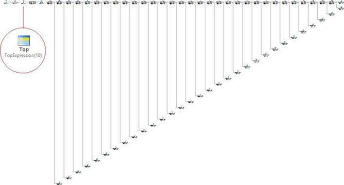
FIGURE 3-13 The harp function.
The beauty of this plan is that the Top operator is the one requesting the rows from the branch to the right of it, and it short-circuits as soon as the requested number of rows is achieved. The Sequence Project and Nested Loops operators, which handle the row-number calculation and cross joins, respectively, respond to the request for rows from the Top operator. As soon as the Top operator stops requesting rows, they stop producing rows. In other words, even though potentially this solution can generate over four billion rows, in practice it generates only the requested number and then short-circuits. Testing the performance of the function on my laptop, it finished generating 10,000,000 numbers in four seconds, with results discarded. That’s not so bad.
The APPLY operator
The APPLY operator is one of the most powerful tools I know of in T-SQL, and yet, it seems to be unnoticed by many. Often when I teach about T-SQL, I ask the students who’s using APPLY and, in many cases, I get only a small percent saying they do. What’s interesting about this operator is that it can be used in very creative ways to solve all kinds of querying tasks.
There are three flavors of APPLY: CROSS APPLY, OUTER APPLY, and implicit APPLY. The following sections describe these flavors.
The CROSS APPLY operator
One way to think of the CROSS APPLY operator is as a hybrid of a cross join and a correlated subquery. Think for a moment of a regular cross join. The inputs can be tables or table expressions, but then the table expressions have to be self-contained. The inner queries are not allowed to be correlated ones. The CROSS APPLY operator is similar to a cross join, only the inner query in the right input is allowed to have correlations to elements from the left input. The left input, like in a cross join, has to be self-contained.
So, T1 CROSS JOIN T2 is equivalent to T1 CROSS APPLY T2. Also, T1 CROSS JOIN (self_contained_query) AS Q is equivalent to T1 CROSS APPLY (self_contained_query) AS Q. However, unlike a cross join, CROSS APPLY allows the right input to be a correlated table subquery, as in T1 CROSS APPLY (SELECT ... FROM T2 WHERE T2.col1 = T1.col1) AS Q. This means that for every row in T1, Q is evaluated separately based on the current value in T1.col1.
Interestingly, standard SQL doesn’t support the APPLY operator but has a similar feature called a lateral derived table. The standard’s parallel to T-SQL’s CROSS APPLY is a CROSS JOIN with a lateral derived table, allowing the right table expression to be a correlated one. So what in T-SQL is expressed as T1 CROSS APPLY (SELECT ... FROM T2 WHERE T2.col1 = T1.col1) AS Q, in standard SQL is expressed as T1 CROSS JOIN LATERAL (SELECT ... FROM T2 WHERE T2.col1 = T1.col1) AS Q.
To demonstrate a practical use case for CROSS APPLY, recall the earlier discussion in this chapter about the top N per group task. The specific example was filtering the most recent orders per customer. The order for the filter was based on orderdate descending with orderid descending used as the tiebreaker. I suggested creating the following POC index to support your solution:
CREATE UNIQUE INDEX idx_poc
ON Sales.Orders(custid, orderdate DESC, orderid DESC)
INCLUDE(empid);
I used the following solution based on a regular correlated subquery:
SELECT orderid, orderdate, custid, empid
FROM Sales.Orders
WHERE orderid IN
(SELECT
(SELECT TOP (1) orderid
FROM Sales.Orders AS O
WHERE O.custid = C.custid
ORDER BY orderdate DESC, orderid DESC)
FROM Sales.Customers AS C);
The problem with a regular subquery is that it’s limited to returning only one column. So this solution used a subquery to return the qualifying order ID per customer, but then another layer was needed with a query against Orders to retrieve the rest of the order information per qualifying order ID. So the plan for this solution shown earlier in Figure 3-3 involved a seek in the POC index per customer to retrieve the qualifying order ID, and another seek per customer in the POC index to retrieve the rest of the order information.
Because CROSS APPLY allows you to apply a correlated table expression, you’re not limited to returning only one column. So you can simplify the solution by removing the need for the extra layer, and instead of doing two seeks per customer, do only one. Here’s what the solution using the CROSS APPLY operator looks like (this time requesting the three most recent orders per customer):
SELECT C.custid, A.orderid, A.orderdate, A.empid
FROM Sales.Customers AS C
CROSS APPLY ( SELECT TOP (3) orderid, orderdate, empid
FROM Sales.Orders AS O
WHERE O.custid = C.custid
ORDER BY orderdate DESC, orderid DESC ) AS A;
It’s both simpler than the previous one and more efficient, as can be seen in the query plan shown in Figure 3-14.
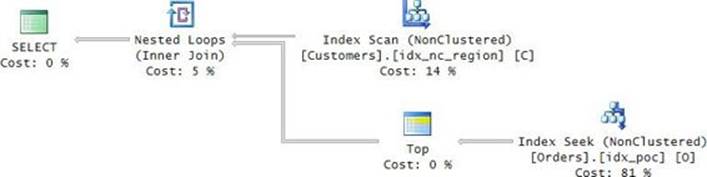
FIGURE 3-14 Plan for a query with the CROSS APPLY operator.
In this example, the inner query is quite simple, so it’s no big deal to embed it directly. But in cases where the inner query is more complex, you would probably want to encapsulate it in an inline TVF, like so:
IF OBJECT_ID(N'dbo.GetTopOrders', N'IF') IS NOT NULL DROP FUNCTION dbo.GetTopOrders;
GO
CREATE FUNCTION dbo.GetTopOrders(@custid AS INT, @n AS BIGINT)
RETURNS TABLE
AS
RETURN
SELECT TOP (@n) orderid, orderdate, empid
FROM Sales.Orders
WHERE custid = @custid
ORDER BY orderdate DESC, orderid DESC;
GO
Then you can replace the correlated table expression with a call to the function, passing C.custid as the input customer ID (the correlation) and 3 as the number of rows to filter per customer, like so:
SELECT C.custid, A.orderid, A.orderdate, A.empid
FROM Sales.Customers AS C
CROSS APPLY dbo.GetTopOrders( C.custid, 3 ) AS A;
You can find a more extensive coverage of efficient handling of the top N per group task in Chapter 5.
The OUTER APPLY operator
The CROSS APPLY operator has something in common with an inner join in that left rows that don’t have matches on the right side are discarded. So, in the previous query, customers who didn’t place orders were discarded. Similar to a left outer join operator, which preserves all left rows, there’s an OUTER APPLY operator that preserves all left rows. Like with an outer join, the OUTER APPLY operator uses NULLs as placeholders for nonmatches on the right side.
As an example, to alter the last query to preserve all customers, replace CROSS APPLY with OUTER APPLY, like so:
SELECT C.custid, A.orderid, A.orderdate, A.empid
FROM Sales.Customers AS C
OUTER APPLY dbo.GetTopOrders( C.custid, 3 ) AS A;
This time, the output includes customers who didn’t place orders:
custid orderid orderdate empid
----------- ----------- ---------- -----------
1 11011 2015-04-09 3
1 10952 2015-03-16 1
1 10835 2015-01-15 1
2 10926 2015-03-04 4
2 10759 2014-11-28 3
2 10625 2014-08-08 3
...
22 NULL NULL NULL
...
57 NULL NULL NULL
58 11073 2015-05-05 2
58 10995 2015-04-02 1
58 10502 2014-04-10 2
...
As mentioned, standard SQL’s parallel to the T-SQL-specific APPLY operator is called a lateral derived table. I described the parallel to the CROSS APPLY operator in the previous section. As for the parallel to OUTER APPLY, what in T-SQL is expressed as T1 OUTER APPLY (SELECT ... FROM T2 WHERE T2.col1 = T1.col1) AS Q, in standard SQL is expressed as T1 LEFT OUTER JOIN LATERAL (SELECT ... FROM T2 WHERE T2.col1 = T1.col1) AS Q ON 1 = 1.
Implicit APPLY
The documented variations of the APPLY operator are the aforementioned CROSS APPLY and OUTER APPLY ones. There is another variation that involves doing something similar to what you do with the explicit APPLY operator, but without using the APPLY keyword in your code. I refer to this variation as implicit APPLY. An implicit APPLY involves using a subquery and, within it, querying a table function to which you pass columns from the outer table as inputs. This is probably best explained through an example.
Consider the GetTopOrders function you used in the previous sections to return the requested number of most recent orders for the requested customer. Suppose you want to compute for each customer from the Customers table the distinct count of employees who handled the customer’s 10 most recent orders. You want to reuse the logic encapsulated in the GetTopOrders function, so you do the following: you query the Customers table; you use a subquery to apply the function to the outer customer to return its 10 most recent orders; finally, you compute the distinct count of employees who handled those orders. Here’s the implementation of this logic in T-SQL:
SELECT C.custid,
( SELECT COUNT(DISTINCT empid) FROM dbo.GetTopOrders( C.custid, 10 ) ) AS numemps
FROM Sales.Customers AS C;
Notice that nowhere does the code mention the APPLY keyword explicitly, but clearly the code in the subquery applies the table function to each outer customer. This code generates the following output:
custid numemps
----------- -----------
1 4
2 3
3 4
4 4
5 6
6 5
7 6
8 2
9 7
11 7
...
It’s easy to see why the term implicit APPLY is appropriate here. Interestingly, before the explicit APPLY operator was added to SQL Server, you couldn’t use the implicit APPLY functionality, either. In other words, the implicit functionality was added thanks to the addition of the explicit operator.
Reuse of column aliases
As discussed in Chapter 1, one of the annoying things about SQL is that if you define a column alias in the SELECT clause of a query, you’re not allowed to refer to it in most query clauses. The only exception is the ORDER BY clause because it’s the only clause that is logically evaluated after the SELECT clause.
There is an elegant trick you can do when using the APPLY operator that solves the problem. Remember that APPLY is a table operator, and table operators are evaluated in the FROM clause of the query. Because the FROM clause is the first clause to be evaluated logically, any aliases you create in it become visible to the rest of the query clauses. Furthermore, because each table operator starts a new series of logical query-processing steps, aliases defined by one table operator are visible to subsequent table operators.
With this in mind, using the APPLY operator you can apply a derived table that defines aliases for expressions based on columns from the left table. The derived table can be based on a SELECT query without a FROM clause, or the VALUES clause, like so:
FROM T1 APPLY ( VALUES(<expressions_based_on_columns_in_T1>) ) AS A(<aliases>)
As an example, consider the following query:
SELECT orderid, orderdate
FROM Sales.Orders
CROSS APPLY ( VALUES( YEAR(orderdate) ) ) AS A1(orderyear)
CROSS APPLY ( VALUES( DATEFROMPARTS(orderyear, 1, 1),
DATEFROMPARTS(orderyear, 12, 31) )
) AS A2(beginningofyear, endofyear)
WHERE orderdate IN (beginningofyear, endofyear);
This query is issued against the Orders table. It is supposed to return only orders placed at the beginning or end of the year. The query uses one CROSS APPLY operator to define the alias orderyear for the expression YEAR(orderdate). It then uses a second CROSS APPLY operator to define the aliases beginningofyear and endofyear for the expressions DATEFROMPARTS(orderyear, 1, 1) and DATEFROMPARTS(orderyear, 12, 31), respectively. The query then filters only the rows where the orderdate value is equal to either the beginningofyear value or the endofyearvalue.
This query generates the following output:
orderid orderdate
----------- ----------
10399 2013-12-31
10400 2014-01-01
10401 2014-01-01
10806 2014-12-31
10807 2014-12-31
10808 2015-01-01
10809 2015-01-01
10810 2015-01-01
From an optimization perspective, this trick doesn’t have a negative performance impact because the expressions in the derived tables get inlined. Internally, after inlining the expressions, the preceding query becomes equivalent to the following query:
SELECT orderid, orderdate
FROM Sales.Orders
WHERE orderdate IN
(DATEFROMPARTS(YEAR(orderdate), 1, 1), DATEFROMPARTS(YEAR(orderdate), 12, 31));
The plans for both queries are the same.
Note that this particular example is pretty simple and is used mainly for illustration purposes. It’s so simple that the benefit in reusing column aliases here is questionable. But this trick becomes extremely handy when the computations are much longer and more complex.
As mentioned, you can use the APPLY operator in creative ways to solve a wide variety of problems. You can find examples in the Microsoft Virtual Academy (MVA) seminar “Boost Your T-SQL with the APPLY Operator” here: http://www.microsoftvirtualacademy.com/training-courses/boost-your-t-sql-with-the-apply-operator.
When you’re done practicing with the APPLY examples, run the following code for cleanup:
DROP INDEX idx_poc ON Sales.Orders;
Joins
The join is by far the most frequently used type of table operator and one of the most commonly used features in SQL in general. Most queries involve combining data from multiple tables, and one of the main tools used for this purpose is a join.
This section covers the fundamental join types (cross, inner, and outer), self, equi, and nonequi joins. It also covers logical and optimization aspects of multi-join queries, semi joins, and anti semi joins, as well as join algorithms. The section concludes with coverage of a common task called separating elements and demonstrates an efficient solution for the task based on joins.
Cross join
Between the three fundamental join types (cross, inner, and outer), the first is the simplest, although it is less commonly used than the others. A cross join produces a Cartesian product of the two input tables. If one table contains M rows and the other N rows, you get a result with M × Nrows.
In terms of syntax, standard SQL (as well as T-SQL) supports two syntaxes for cross joins. One is an older syntax in which you specify a comma between the table names, like so:
SELECT E1.firstname AS firstname1, E1.lastname AS lastname1,
E2.firstname AS firstname2, E2.lastname AS lastname2
FROM HR.Employees AS E1, HR.Employees AS E2;
Another is a newer syntax that was added in the SQL-92 standard, in which you specify a keyword indicating the join type (CROSS, in our case) followed by the JOIN keyword between the table names, like so:
SELECT E1.firstname AS firstname1, E1.lastname AS lastname1,
E2.firstname AS firstname2, E2.lastname AS lastname2
FROM HR.Employees AS E1
CROSS JOIN HR.Employees AS E2;
Both syntaxes are standard, and both are supported by T-SQL. There’s neither a logical difference nor an optimization difference between the two. You might wonder, then, why did standard SQL bother creating two different syntaxes if they have the same meaning? The reason for this doesn’t really have anything to do with cross and inner joins; rather, it is related to outer joins. Recall from the discussions in Chapter 1 that an outer join involves a matching predicate, which has a very different role than a filtering predicate. The former defines only which rows from the nonpreserved side of the join match to rows from the preserved side, but it cannot filter out rows from the preserved side. The latter is used as a basic filter and can certainly discard rows from both sides.
The SQL standards committee decided to add support for outer joins in the SQL-92 standard, but they figured that the traditional comma-based syntax doesn’t lend itself to supporting the new type of join. That’s because this syntax doesn’t allow you to define a matching predicate as part of the join table operator, which as mentioned, is supposed to play a different role than the filtering predicate that you specify in the WHERE clause. So they ended up creating the newer syntax with the JOIN keyword with a designated ON clause where you indicate the matching predicate. This newer syntax with the JOIN keyword is commonly referred to as the SQL-92 syntax, and the older comma-based syntax is referred to as the SQL-89 syntax.
To allow a consistent coding style for the different types of joins, the SQL-92 standard also added support for a similar JOIN-keyword-based syntax for cross and inner joins. That’s the history explaining why you now have two standard syntaxes for cross and inner joins and only one standard syntax for outer joins. It is strongly recommended that you stick to using the JOIN-keyword-based syntax across the board. One reason is that it results in a consistent coding style that is so much easier to maintain than a mixed style. Furthermore, the comma-based syntax is more prone to errors, as I will demonstrate later when discussing inner joins.
I’ll demonstrate a couple examples of use cases of cross joins. One is generating sample data, and the other is circumventing an optimization problem related to subqueries.
Suppose you need to generate sample data representing orders. An order has an order ID, was placed on a certain date, was placed by a certain customer, and was handled by a certain employee. You get as inputs the range of order dates as well as the number of distinct customers and employees you need to support. Using the GetNums function in the sample database, you can generate sets of dates, customer IDs, and employee IDs. You perform cross joins between those sets to get all possible combinations and, using a ROW_NUMBER function, compute the order IDs, like so:
DECLARE @s AS DATE = '20150101', @e AS DATE = '20150131',
@numcusts AS INT = 50, @numemps AS INT = 10;
SELECT ROW_NUMBER() OVER(ORDER BY (SELECT NULL)) AS orderid,
DATEADD(day, D.n, @s) AS orderdate, C.n AS custid, E.n AS empid
FROM dbo.GetNums(0, DATEDIFF(day, @s, @e)) AS D
CROSS JOIN dbo.GetNums(1, @numcusts) AS C
CROSS JOIN dbo.GetNums(1, @numemps) AS E;
The unusual order specification ORDER BY (SELECT NULL) in the ROW_NUMBER function is a trick used to compute row numbers based on an arbitrary order. I use this trick when I need to generate unique values and I don’t care about the order in which they are generated.
Note that usually when you generate sample data, you need a more sophisticated solution that results in a more realistic distribution of the data. In reality, you typically don’t have even distribution of order dates, customer IDs, and employee IDs. But sometimes you need a very basic form of sample data for certain tests, and this simple technique can be sufficient for you.
Another use case for cross joins has to do with a certain optimization shortcoming in SQL Server related to subqueries. Consider the following query:
SELECT orderid, val,
val / (SELECT SUM(val) FROM Sales.OrderValues) AS pct,
val - (SELECT AVG(val) FROM Sales.OrderValues) AS diff
FROM Sales.OrderValues;
This query is issued against the OrderValues view. It returns for each order the percent of the current order value out of the grand total as well as the difference from the grand average. The grand total and grand average are computed by scalar aggregate subqueries. It is true that the query refers to the OrderValues view three times, but clearly both subqueries need to operate on the exact same set of values. Unfortunately, currently there’s no logic in the optimizer to avoid the duplication of work by collapsing all matching subqueries into one activity that will feed the same set of values to all aggregate calculations. In our case, the problem is even further magnified because OrderValues is a view. The view joins the Orders and OrderDetails tables, and it groups and aggregates the data to produce order-level information. All of this work is repeated three times in the execution plan for our query, as you can see in Figure 3-15.
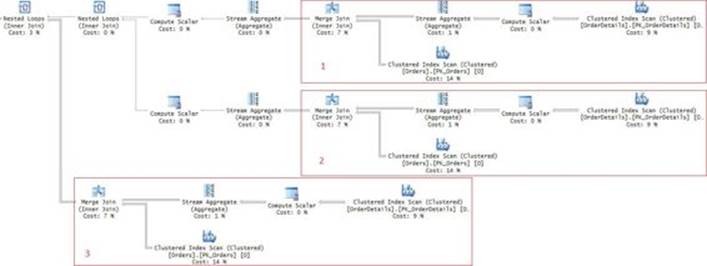
FIGURE 3-15 Work is repeated for every subquery.
The branches marked as 1 and 2 represent the work for the two subqueries feeding the values to the two aggregate calculations. The branch marked as 3 represents the reference to the view in the outer query to obtain the order information—in other words, the detail. As you can imagine, the more aggregates you have, the worse this solution performs. Imagine you had 10 different aggregates to compute. This would require 11 repetitions of the work—10 for the aggregates and one for the detail.
Fortunately, there is a way to avoid the unnecessary repetition of the work. To achieve this, you use one query to compute all aggregates that you need. SQL Server will optimize this query by applying the work only once, feeding the same values to all aggregate calculations. You define a table expression based on that query (call it Aggs) and perform a cross join between the OrderValues view and Aggs. Then, in the SELECT list, you perform all your calculations involving the detail and the aggregates. Here’s the complete solution query:
SELECT orderid, val,
val / sumval AS pct,
val - avgval AS diff
FROM Sales.OrderValues
CROSS JOIN (SELECT SUM(val) AS sumval, AVG(val) AS avgval
FROM Sales.OrderValues) AS Aggs;
Observe the execution plan for this query shown in Figure 3-16.
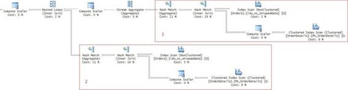
FIGURE 3-16 Avoiding repetition of work with a join.
Notice that this time the work represented by the view happens only once for all aggregates (branch 1) and once for the detail (branch 2). The nice thing with this solution is that it doesn’t matter how many aggregates you have—you will still have only one activity that collects the values for all of them.
You will face a similar problem when you need the calculation to be partitioned. For example, suppose that instead of grand aggregates, you need customer aggregates. In other words, you need to compute the percent of the current order value out of the customer total (not the grand total) and the difference from the customer average. Using the subquery approach, you add correlations, like so:
SELECT orderid, val,
val / (SELECT SUM(val) FROM Sales.OrderValues AS I
WHERE I.custid = O.custid) AS pct,
val - (SELECT AVG(val) FROM Sales.OrderValues AS I
WHERE I.custid = O.custid) AS diff
FROM Sales.OrderValues AS O;
But again, because you’re using subqueries, the work represented by the view will be repeated three times. The solution is similar to the previous one, only instead of using a cross join, you use an inner join and match the customer IDs between the OrderValues view and Aggs, like so:
SELECT orderid, val,
val / sumval AS pct,
val - avgval AS diff
FROM Sales.OrderValues AS O
INNER JOIN (SELECT custid, SUM(val) AS sumval, AVG(val) AS avgval
FROM Sales.OrderValues
GROUP BY custid) AS Aggs
ON O.custid = Aggs.custid;
Inner join
From a logical query-processing perspective, an inner join involves two steps. It starts with a Cartesian product between the two input tables, like in a cross join. It then applies a filter that usually involves matching elements from both sides. From a physical query-processing perspective, of course things can be done differently, provided that the output is correct.
Like with cross joins, inner joins currently have two standard syntaxes. One is the SQL-89 syntax, where you specify commas between the table names and then apply all filtering predicates in the WHERE clause, like so:
SELECT C.custid, C.companyname, O.orderid
FROM Sales.Customers AS C, Sales.Orders AS O
WHERE C.custid = O.custid
AND C.country = N'USA';
As you can see, the syntax doesn’t really distinguish between a cross join and an inner join; rather, it expresses an inner join as a cross join with a filter.
The other syntax is the SQL-92 one, which is more compatible with the standard outer join syntax. You specify the INNER JOIN keywords between the table names (or just JOIN because INNER is the default) and the join predicate in the mandatory ON clause. If you have any additional filters, you can specify them either in the join’s ON clause or in the usual WHERE clause, like so:
SELECT C.custid, C.companyname, O.orderid
FROM Sales.Customers AS C
INNER JOIN Sales.Orders AS O
ON C.custid = O.custid
WHERE C.country = N'USA';
Despite the fact that the ON clause is mandatory in the SQL-92 syntax for inner joins, there is no distinction between a matching predicate and a filtering predicate like in outer joins. Both predicates are treated as filtering predicates. So, even though from a logical query-processing perspective, the WHERE clause is supposed to be evaluated after the FROM clause with all of its joins, the optimizer might very well decide to process the predicates from the WHERE clause before it starts processing the joins in the FROM clause. In fact, if you examine the plans for the two queries just shown, you will notice that in both cases the plan starts with a scan of the clustered index on the Customers table and applies the country filter as part of the scan.
I mentioned earlier that it’s recommended to stick to the SQL-92 syntax for joins and avoid the SQL-89 syntax even though it’s standard for cross and inner joins. I already provided one reason for this recommendation—using one consistent style for all types of joins. Another reason is that the SQL-89 syntax is more prone to errors; specifically, it is more likely you will miss a join predicate and for such a mistake to go unnoticed. With the SQL-92 syntax, you usually specify each join predicate right after the respective join, like so:
FROM T1
INNER JOIN T2
ON T2.col1 = T1.col1
INNER JOIN T3
ON T3.col2 = T2.col2
INNER JOIN T4
ON T4.col3 = T3.col3
With this syntax, the likelihood that you will miss a join predicate is low, and even if you do, the parser will generate an error because the ON clause is mandatory with inner (and outer) joins. Conversely, with the SQL-89 syntax, you specify all table names separated by commas in the FROM clause, and all predicates as a conjunction in the WHERE clause, like so:
FROM T1, T2, T3, T4
WHERE T2.col1 = T1.col1 AND T3.col2 = T2.col2 AND T4.col3 = T3.col3
Clearly the likelihood that you will miss a predicate by mistake is higher, and if you do, you end up with an unintentional cross join.
A common question I get is whether there’s a difference between using the keywords INNER JOIN and just JOIN. There’s none. Standard SQL made inner joins the default because it’s probably the most commonly used type of join. In a similar way, standard SQL made the keyword OUTER optional in outer joins. For example, LEFT OUTER JOIN and LEFT JOIN are equivalent. As for what’s recommended to use, some prefer the full syntax finding it to be clearer. Others prefer the missing syntax because it results in shorter code. I think that what’s more important than whether to use the full or missing syntax is to be consistent between the members of the development team. When different people use different styles, it can be hard to maintain each other’s code. A good idea is to have meetings to discuss styling choices like full versus missing syntax, indentation, casing, and so on, and to come up with a coding style document that everyone must follow. Sometimes people have strong opinions about certain styling aspects based on their personal preferences, so when conflicts arise you can vote to determine which option will prevail. Once everyone starts using a consistent style, it becomes so much easier for different people to maintain the same code.
Outer join
From a logical query-processing perspective, outer joins start with the same two steps as inner joins. But in addition, they have a third logical step that ensures that all rows from the table or tables that you mark as preserved are returned, even if they don’t have any matches in the other table based on the join predicate. Using the keywords LEFT (or LEFT OUTER), RIGHT, or FULL, you mark the left table, right table, or both tables as preserved. Output rows representing nonmatches (aka outer rows) have NULLs used as placeholders in the nonpreserved side’s columns.
As an example, the following query returns customers and their orders, including customers with no orders:
SELECT C.custid, C.companyname, C.country,
O.orderid, O.shipcountry
FROM Sales.Customers AS C
LEFT OUTER JOIN Sales.Orders AS O
ON C.custid = O.custid;
In outer joins, the role of the predicate in the ON clause is different than in inner joins. With the latter, it serves as a simple filtering tool, whereas with the former it serves as a more sophisticated matching tool. All rows from the preserved side will be returned whether they find matching rows based on the predicate or not. If you need any simple filters to be applied, you specify those in the WHERE clause. For example, a classic way to identify only nonmatches is to use an outer join and add a WHERE clause that filters only the rows that have a NULL in a column from the nonpreserved side that doesn’t allow NULLs normally. The primary key column is a good choice for this purpose. For example, the following query returns only customers who didn’t place orders:
SELECT C.custid, C.companyname, O.orderid
FROM Sales.Customers AS C
LEFT OUTER JOIN Sales.Orders AS O
ON C.custid = O.custid
WHERE O.orderid IS NULL;
It’s far more common to see people using left outer joins than right outer ones. It could be because most people tend to specify referenced tables before referencing ones in the query, and usually the referenced table is the one that can have rows with no matches in the referencing one. It’s true that in a single join case such as T1 LEFT OUTER JOIN T2 you can express the same thing with a symmetric T2 RIGHT OUTER JOIN T1. However, in certain more complex cases with multiple joins involved, you will find that using a right outer join enables a simpler solution than using left outer joins. I’ll demonstrate such a case shortly in the “Multi-join queries” section.
Self join
A self join is a join between multiple instances of the same table. As an example, the following query matches employees with their managers, who are also employees:
SELECT E.firstname + ' ' + E.lastname AS emp, M.firstname + ' ' + M.lastname AS mgr
FROM HR.Employees AS E
LEFT OUTER JOIN HR.Employees AS M
ON E.mgrid = M.empid;
What’s special about self joins is that it’s mandatory to alias the instances of the table differently; otherwise, you end up with duplicate column names, including the table prefixes.
From an optimization perspective, the optimizer looks at the two instances as two different tables. For example, it can use different indexes for each of the instances. In the query plan, you can identify in each physical object that is accessed which instance it represents based on the table alias you assigned to it.
Equi and non-equi joins
The terms equi joins and non-equi joins refer to the kind of operator you use in the join predicate. When you use an equality operator, like in the vast majority of the queries, the join is referred to as an equi join. When you use an operator other than equality, the join is referred to as a non-equi join.
As an example, the following query uses a non-equi join with a less than (<) operator to identify unique pairs of employees:
SELECT E1.empid, E1.lastname, E1.firstname, E2.empid, E2.lastname, E2.firstname
FROM HR.Employees AS E1
INNER JOIN HR.Employees AS E2
ON E1.empid < E2.empid;
If you’re wondering why you should use a non-equi join here rather than a cross join, that’s because you don’t want to get the self-pairs (same employee x, x on both sides) and you don’t want to get mirrored pairs (x, y and also y, x). If you want to produce unique triples, simply add another non-equi join to a third instance of the table (call it E3), with the join predicate E2.empid < E3.empid.
From an optimization perspective, there’s relevance to identifying the join as an equi or non-equi one. Later, the chapter covers the optimization of joins with the join algorithms nested loop, merge, and hash. Nested loops is the only algorithm supported with non-equi joins. Merge and hash require an equi-join or, more precisely, at least one predicate that is based on an equality operator.
Multi-join queries
Multi-join queries are queries with multiple joins (what a surprise). There are a number of interesting considerations concerning such queries, some optimization related and others related to the logical treatment.
As an example, the following query joins five tables to return customer-supplier pairs that had activity together:
SELECT DISTINCT C.companyname AS customer, S.companyname AS supplier
FROM Sales.Customers AS C
INNER JOIN Sales.Orders AS O
ON O.custid = C.custid
INNER JOIN Sales.OrderDetails AS OD
ON OD.orderid = O.orderid
INNER JOIN Production.Products AS P
ON P.productid = OD.productid
INNER JOIN Production.Suppliers AS S
ON S.supplierid = P.supplierid;
The customer company name is obtained from the Customers table. The Customers table is joined with the Orders table to find the headers of the orders that the customers placed. The result is joined with OrderDetails to find the order lines within those orders. The order lines contain the IDs of the products that were ordered. The result is joined with Products, where the IDs of the suppliers of those products are found. Finally, the result is joined with Suppliers to get the supplier company name.
Because the same customer-supplier pair can appear more than once in the result, the query has a DISTINCT clause to eliminate duplicates. Here there was a good reason to use DISTINCT. Note, however, that if you see excessive use of DISTINCT in someone’s join queries, it could indicate that they don’t correctly understand the relationships in the data model. When joining tables based on incorrect relationships, you can end up with duplicates, and the use of DISTINCT in such a case could be an attempt to hide those.
The following sections discuss aspects of the physical and logical processing of this query.
Controlling the physical-join evaluation order
When discussing logical query processing in Chapter 1, I explained that table operators are evaluated from left to right. That’s the case from a logical-processing standpoint. However, from a physical-processing standpoint, under certain conditions the order can be altered without changing the meaning of the query. With outer joins, changing the order can change the meaning, and this is something the optimizer isn’t allowed to do. But with inner and cross joins, changing the order doesn’t change the meaning. So, with those, the optimizer will apply join-ordering optimization. It will explore different join orders and pick the one from those that according to its estimates is supposed to be the fastest.
As an example, our multi-join query got the plan in Figure 3-17, showing that the physical join order is different than the logical one.
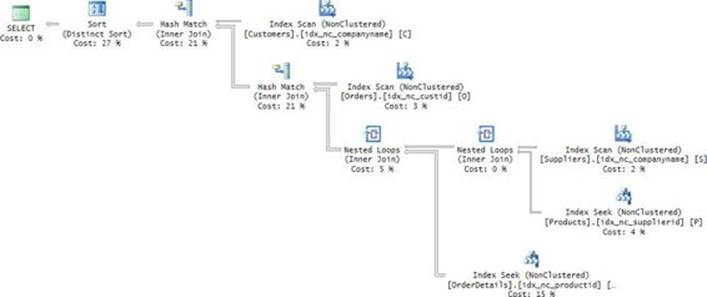
FIGURE 3-17 Plan for a multi-join query.
Observe the order in the plan is as follows: Customers join ( Orders join ( ( Suppliers join Products ) join OrderDetails ) ). For illustration purposes, the following query applies logical join ordering that reflects the physical ordering in Figure 3-17:
SELECT DISTINCT C.companyname AS customer, S.companyname AS supplier
FROM Sales.Customers AS C
INNER JOIN ( Sales.Orders AS O
INNER JOIN ( Production.Suppliers AS S
INNER JOIN Production.Products AS P
ON P.supplierid = S.supplierid
INNER JOIN Sales.OrderDetails AS OD
ON OD.productid = P.productid )
ON OD.orderid = O.orderid )
ON O.custid = C.custid;
There are a number of reasons that could lead the optimizer to choose a suboptimal join order. Like with other suboptimal choices, join ordering choices can be affected by inaccurate cardinality estimates.
Furthermore, the theoretical number of possible join orders, or join trees, can be very large even with a small number of tables. Benjamin Nevarez explains this in “Optimizing Join Orders” here: http://www.benjaminnevarez.com/2010/06/optimizing-join-orders/. With N tables, the number of possible trees is (2N – 2)! / (N – 1)!, where ! is factorial. As an example, in our case we have 5 tables resulting in 1,680 possible trees. With 10 tables, the number is 17,643,225,600! Here the ! is for amazement, not to represent factorial, thank goodness. As you might realize, if the optimizer actually tried to explore all possible join trees, the optimization process would take too long and become counterproductive. So the optimizer does a number of things to reduce the optimization time. It computes cost-based and time-based thresholds based on the sizes of the tables involved, and if one of them is reached, optimization stops. The optimizer also normally doesn’t consider bushy join trees, where results of joins are joined; such trees represent the majority of the trees. What all this means is that the optimizer might not come up with the truly optimal join order.
If you suspect that’s the case and want to force the optimizer to use a certain order, you can do so by typing the joins in the order you think is optimal and adding the FORCE ORDER query hint, like so:
SELECT DISTINCT C.companyname AS customer, S.companyname AS supplier
FROM Sales.Customers AS C
INNER JOIN Sales.Orders AS O
ON O.custid = C.custid
INNER JOIN Sales.OrderDetails AS OD
ON OD.orderid = O.orderid
INNER JOIN Production.Products AS P
ON P.productid = OD.productid
INNER JOIN Production.Suppliers AS S
ON S.supplierid = P.supplierid
OPTION (FORCE ORDER);
This hint is certainly good as a troubleshooting tool because you can use it to test the performance of different orders and see if the optimizer, indeed, made a suboptimal choice. The problem with using such a hint in production code is that it makes this part of optimization static. Normally, changes in indexing, data characteristics, and other factors can result in a change in the optimizer’s join ordering choice, but obviously not when the hint is used. So the hint is good to use as a troubleshooting tool and sometimes as a short, temporary solution in production in critical cases. However, it’s usually not good to use as a long-term solution. For example, suppose the cause for the suboptimal join-ordering choice was a bad cardinality estimate. When you have the time to do more thorough research of the problem, I hope you can find ways to help the optimizer come up with more accurate estimates that naturally lead to a more optimal plan.
Controlling the logical-join evaluation order
You just saw how to control physical join ordering. There are also cases where you need to control logical join ordering to achieve a certain change in the meaning of the query. As an example, consider the query that returns customer-supplier pairs from the previous section:
SELECT DISTINCT C.companyname AS customer, S.companyname AS supplier
FROM Sales.Customers AS C
INNER JOIN Sales.Orders AS O
ON O.custid = C.custid
INNER JOIN Sales.OrderDetails AS OD
ON OD.orderid = O.orderid
INNER JOIN Production.Products AS P
ON P.productid = OD.productid
INNER JOIN Production.Suppliers AS S
ON S.supplierid = P.supplierid;
This query returns 1,236 rows. All joins in the query are inner joins. This means that customers who didn’t place any orders aren’t returned. There are two such customers in our sample data. Suppose you need to change the solution to include customers without orders. The intuitive thing to do is change the type of join between Customers and Orders to a left outer join, like so:
SELECT DISTINCT C.companyname AS customer, S.companyname AS supplier
FROM Sales.Customers AS C
LEFT OUTER JOIN Sales.Orders AS O
ON O.custid = C.custid
INNER JOIN Sales.OrderDetails AS OD
ON OD.orderid = O.orderid
INNER JOIN Production.Products AS P
ON P.productid = OD.productid
INNER JOIN Production.Suppliers AS S
ON S.supplierid = P.supplierid;
However, if you run the query, you will notice that it still returns the same result as before. Logically, the left outer join between Customers and Orders returns the two customers who didn’t place orders with NULLs in the order attributes. Then when joining the result with OrderDetails using an inner join, those outer rows are eliminated. That’s because when comparing the NULL marks in the O.orderid column in those rows with any OD.orderid value, the result is the logical value unknown. You can generalize this case and say that any left outer join that is subsequently followed by an inner join or a right outer join causes the left outer join to effectively become an inner join. That’s assuming that you compare the NULL elements from the nonpreserved side of the left outer join with elements from another table. In fact, if you look at the execution plan of the query, you will notice that, indeed, the optimizer converted the left outer join to an inner join.
A common way for people to attempt to solve the problem is to make all joins left outer joins, like so:
SELECT DISTINCT C.companyname AS customer, S.companyname AS supplier
FROM Sales.Customers AS C
LEFT OUTER JOIN Sales.Orders AS O
ON O.custid = C.custid
LEFT OUTER JOIN Sales.OrderDetails AS OD
ON OD.orderid = O.orderid
LEFT OUTER JOIN Production.Products AS P
ON P.productid = OD.productid
LEFT OUTER JOIN Production.Suppliers AS S
ON S.supplierid = P.supplierid;
There are two problems with this solution. One problem is that you actually changed the meaning of the query from the intended one. You were after a left outer join between Customers and the result of the inner joins between the remaining tables. Rows without matches in the remaining tables aren’t supposed to be preserved; however, with this solution, if they are left rows, they will be preserved. The other problem is that the optimizer has less flexibility in altering the join order when dealing with outer joins. Pretty much the only flexibility that it does have is to change T1 LEFT OUTER JOIN T2 to T2 RIGHT OUTER JOIN T1.
A better solution is to start with the inner joins between the tables besides Customers and then to apply a right outer join with Customers, like so:
SELECT DISTINCT C.companyname AS customer, S.companyname AS supplier
FROM Sales.Orders AS O
INNER JOIN Sales.OrderDetails AS OD
ON OD.orderid = O.orderid
INNER JOIN Production.Products AS P
ON P.productid = OD.productid
INNER JOIN Production.Suppliers AS S
ON S.supplierid = P.supplierid
RIGHT OUTER JOIN Sales.Customers AS C
ON C.custid = O.custid;
Now the solution is both semantically correct and leaves more flexibility to the optimizer to apply join-ordering optimization. This query returns 1,238 rows, which include the two customers who didn’t place orders.
There’s an even more elegant solution that allows you to express the joins in a manner similar to the way you think of the task. Remember you want to apply a left outer join between Customers and a unit representing the result of the inner joins between the remaining tables. To define such a unit, simply enclose the inner joins in parentheses and move the join predicate that relates Customers and that unit after the parentheses, like so:
SELECT DISTINCT C.companyname AS customer, S.companyname AS supplier
FROM Sales.Customers AS C
LEFT OUTER JOIN
( Sales.Orders AS O
INNER JOIN Sales.OrderDetails AS OD
ON OD.orderid = O.orderid
INNER JOIN Production.Products AS P
ON P.productid = OD.productid
INNER JOIN Production.Suppliers AS S
ON S.supplierid = P.supplierid)
ON O.custid = C.custid;
Curiously, the parentheses are not really required. If you remove them and run the code, you will see it runs successfully and returns the correct result. What really makes the difference is the parentheses-like arrangement of the units and the placement of the ON clauses reflecting this arrangement. Simply make sure that the ON clause that is supposed to relate two units appears right after them; otherwise, the query will not be a valid one. With this in mind, following is another valid arrangement of the units, achieving the desired result for our task:
SELECT DISTINCT C.companyname AS customer, S.companyname AS supplier
FROM Sales.Customers AS C
LEFT OUTER JOIN Sales.Orders AS O
INNER JOIN Sales.OrderDetails AS OD
INNER JOIN Production.Products AS P
INNER JOIN Production.Suppliers AS S
ON S.supplierid = P.supplierid
ON P.productid = OD.productid
ON OD.orderid = O.orderid
ON O.custid = C.custid;
I find that using parentheses accompanied with adequate indentation results in much clearer code, so I recommend using them even though they are not required.
Earlier I mentioned that one of the heuristics the optimizer uses to reduce optimization time is to not consider bushy plans that involve joins between results of joins. If you suspect that such a bushy plan is the most efficient and want the optimizer to use it, you need to force it. The way you achieve this is by defining two units, each based on a join with the respective ON clause, followed by an ON clause that relates the two units. You also need to specify the FORCE ORDER query option.
Following is an example of forcing such a bushy plan:
SELECT DISTINCT C.companyname AS customer, S.companyname AS supplier
FROM Sales.Customers AS C
INNER JOIN
(Sales.Orders AS O INNER JOIN Sales.OrderDetails AS OD
ON OD.orderid = O.orderid)
INNER JOIN
(Production.Products AS P INNER JOIN Production.Suppliers AS S
ON S.supplierid = P.supplierid)
ON P.productid = OD.productid
ON O.custid = C.custid
OPTION (FORCE ORDER);
Here you have one unit (call it U1) based on a join between Orders and OrderDetails. You have another unit (call it U2) based on a join between Products and Suppliers. Then you have a join between the two units (call the result U1-2). Then you have a join between Customers and U1-2. The execution plan for this query is shown in Figure 3-18.
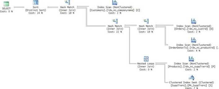
FIGURE 3-18 Bushy plan.
Observe that the desired bushy layout was achieved in the plan.
Semi and anti semi joins
Normally, a join matches rows from two tables and returns elements from both sides. What makes a join a semi join is that you return elements from only one of the sides. The side you return the elements from determines whether it’s a left or right semi join.
As an example, consider a request to return the customer ID and company name of customers who placed orders. You return information only from the Customers table, provided that a matching row is found in the Orders table. Considering the Customers table as the left table, the operation is a left semi join. There are a number of ways to implement the task. One is to use an inner join and apply a DISTINCT clause to remove duplicate customer info, like so:
SELECT DISTINCT C.custid, C.companyname
FROM Sales.Customers AS C
INNER JOIN Sales.Orders AS O
ON O.custid = C.custid;
Another is to use the EXISTS predicate, like so:
SELECT custid, companyname
FROM Sales.Customers AS C
WHERE EXISTS(SELECT *
FROM Sales.Orders AS O
WHERE O.custid = C.custid);
Both queries get the same plan. Of course, there are more ways to achieve the task.
An anti semi join is one in which you return elements from one table if a matching row cannot be found in a related table. Also here, depending on whether you return information from the left table or the right one, the join is either a left or right anti semi join. As an example, a request to return customers who did not place orders is fulfilled with a left anti semi join operation.
There are a number of classic ways to achieve such an anti semi join. One is to use a left outer join between Customers and Orders and filter only outer rows, like so:
SELECT C.custid, C.companyname
FROM Sales.Customers AS C
LEFT OUTER JOIN Sales.Orders AS O
ON O.custid = C.custid
WHERE O.orderid IS NULL;
Another is to use the NOT EXISTS predicate, like so:
SELECT custid, companyname
FROM Sales.Customers AS C
WHERE NOT EXISTS(SELECT *
FROM Sales.Orders AS O
WHERE O.custid = C.custid);
Curiously, it appears that currently the optimizer doesn’t have logic to detect the outer join solution as actually applying an anti semi join, but it does with the NOT EXISTS solution. This can be seen in the execution plans for these queries shown in Figure 3-19.
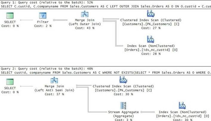
FIGURE 3-19 Plans for anti semi join solutions.
Of course, there are a number of additional ways to implement anti semi joins. The ones I showed are two classic ones.
Join algorithms
Join algorithms are the physical join strategies SQL Server uses to process joins. SQL Server supports three join algorithms: nested loops, merge, and hash. Nested loops is the oldest of the three algorithms and the fallback when the others can’t be used. For example, cross join can be processed only with nested loops. Merge and hash require the join to be an equi join or, more precisely, to have at least one join predicate that is based on an equality operator.
In the graphical query plan, the join operator has a distinct icon for each algorithm. In addition, the Physical Operation property indicates the join algorithm (Nested Loops, Hash Match, or Merge Join), and the Logical Operation property indicates the logical join type (Inner Join, Left Outer Join, Left Anti Semi Join, and so on). Also, the physical algorithm name appears right below the operator, and the logical join type appears below the algorithm name in parentheses.
The following sections describe the individual join algorithms, the circumstances in which they tend to be efficient, and indexing guidelines to support them.
Nested loops
The nested loops algorithm is pretty straightforward. It executes the outer (top) input only once and, using a loop, it executes the inner (bottom) input for each row from the outer input to identify matches.
Nested loops tends to perform well when the outer input is small and the inner input has an index with the key list based on the join column plus any additional filtered columns, if relevant. Whether it’s critical for the index to be a covering one depends on how many matches you get in total. If the total number of matches is small, a few lookups are not too expensive and therefore the index doesn’t have to be a covering one. If the number of matches is large, the lookups become expensive, and then it becomes more critical to avoid them by making the index a covering one.
As an example, consider the following query:
USE PerformanceV3;
SELECT C.custid, C.custname, O.orderid, O.empid, O.shipperid, O.orderdate
FROM dbo.Customers AS C
INNER JOIN dbo.Orders AS O
ON O.custid = C.custid
WHERE C.custname LIKE 'Cust_1000%'
AND O.orderdate >= '20140101'
AND O.orderdate < '20140401';
Currently, the tables don’t have good indexing to support an efficient nested loops join. Because the smaller side (Customers, in our case) is usually used as the outer input and is executed only once, it’s not that critical to support it with a good index. In the worst case, the small table gets fully scanned. The far more critical index here is on the bigger side (Orders, in our case). Nevertheless, if you want to avoid a full scan of the Customers table, you can prepare an index on the filtered column custname as the key and include the custid column for coverage. As for the ideal index on the Orders table, think of the work involved in a single iteration of the loop for some customer X. It’s like submitting the following query:
SELECT orderid, empid, shipperid, orderdate
FROM dbo.Orders
WHERE custid = X
AND orderdate >= '20140101'
AND orderdate < '20140401';
Because you have one equality predicate and one range predicate, it’s quite straightforward to come up with an ideal index here. You define the index with the key list based on custid and orderdate, and you include the remaining columns (orderid, empid, and shipperid) for coverage. Remember the discussions about multiple range predicates in Chapter 2? When you have both an equality predicate and a range predicate, you need to define the index key list with the equality column first. This way, qualifying rows will appear in a consecutive range in the index leaf. That’s not going to be the case if you define the key list with the range column first.
Run the following code to create optimal indexing for our query:
CREATE INDEX idx_nc_cn_i_cid ON dbo.Customers(custname) INCLUDE(custid);
CREATE INDEX idx_nc_cid_od_i_oid_eid_sid
ON dbo.Orders(custid, orderdate) INCLUDE(orderid, empid, shipperid);
Now run the query and examine the query plan shown in Figure 3-20.
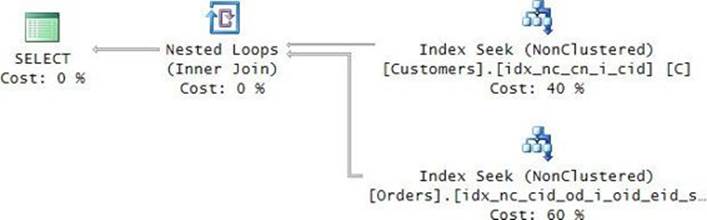
FIGURE 3-20 Plan with a nested loops algorithm.
As you can see, the optimizer chose to use the nested loops algorithm with the smaller table, Customers, as the outer input and the bigger table, Orders, as the inner input. The plan performs a seek and a range scan in the covering index on Customers to retrieve qualifying customers. (There are 11 in our case.) Then, using a loop, the plan performs for each customer a seek and a range scan in the covering index on Orders to retrieve matching orders for the current customer. There are 30 matching orders in total.
Next, I’ll discuss the effects that different changes to the query will have on its optimization.
As mentioned, if you have a small number of matches in total, it’s not that critical for the index on the inner table to be a covering one. You can test such a case by adding O.filler to the query’s SELECT list. The plan will still use the nested loops algorithm, but it will add key lookups to retrieve the column filler from the clustered index because it’s not part of the index idx_nc_cid_od_i_oid_eid_sid. When you’re done testing, make sure you remove the column O.filler from the query before applying the next change.
When enough rows are returned from the outer input, the optimizer usually applies a prefetch (a read-ahead) to speed up the executions of inner input. Usually, the optimizer considers a prefetch when it estimates that more than a couple of dozen rows will be returned from the outer input. The plan for our current query doesn’t involve a prefetch because the optimizer estimates that only a few rows will be returned from Customers. But if you change the query filter against Customers from C.custname LIKE ‘Cust_1000%’ to C.custname LIKE ‘Cust_100%’, it will use a prefetch. After applying the change, you will find that the Nested Loops operator has a property called WithUnorderedPrefetch, which is set to True. The reason it’s an unordered prefetch is that there’s no relevance to returning the rows sorted by the customer IDs. If you add ORDER BY custid to the query, the property will change to WithOrderedPrefetch. When you’re done testing, make sure to revert back to the original query before applying the next change.
I mentioned that the Nested Loops operator is usually efficient when the outer input is small. Change the filter against Customers to C.custname LIKE ‘Cust_10%’. Now the estimated number of matches from Customers increases from just a few to over a thousand, and the optimizer changes its choice of the join algorithm to hash.
There’s an interesting technique the optimizer can use when the plan is a parallel one but there are only a few outer rows. In such a case, without optimizer intervention the work could be unevenly distributed to the different threads. Therefore, when the optimizer detects a case of a few outer rows, it adds a Redistribute Streams operator after obtaining the rows from the outer input. This operator redistributes the rows between the threads more evenly.
Merge
The merge algorithm requires both inputs to be sorted by the join column. It then merges the two like a zipper. If the join is a one-to-many one, as is likely to be the case in most queries, there’s only one pass over each input. If the join type is a many-to-many one, one input is scanned once and the other involves rewinds.
Generally, there are two ways for the optimizer to get a sorted input. If the data is already sorted in an index, the optimizer can use an index order scan. The other way is by adding an explicit sort operation to the plan, but then there’s the extra cost that is associated with sorting.
Consider the following query as an example of obtaining sorted data from indexes:
SELECT C.custid, C.custname, O.orderid, O.empid, O.shipperid, O.orderdate
FROM dbo.Customers AS C
INNER JOIN dbo.Orders AS O
ON O.custid = C.custid;
The PK_Customers index on the Customers table is a clustered index defined on custid as the key. So the data from Customers is covered by the index and sorted like the merge join algorithm requires. The nonclustered index idx_nc_cid_od_i_oid_eid_sid on Orders that you created for the example in the “Nested loops” section is quite efficient for a merge join. It has the data sorted by custid as the leading key, and it covers the elements in the query from Orders. The conditions are optimal for a merge join algorithm; therefore, the optimizer uses this strategy, as you can see in the plan for our query shown in Figure 3-21.
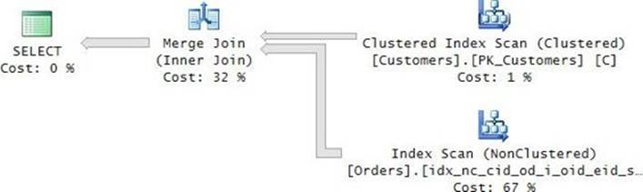
FIGURE 3-21 Plan with a merge algorithm.
As an example for a merge join involving explicit sorting, consider the following query:
SELECT C.custid, C.custname, O.orderid, O.empid, O.shipperid, O.orderdate
FROM dbo.Customers AS C
INNER JOIN dbo.Orders AS O
ON O.custid = C.custid
WHERE O.orderdate >= '20140101'
AND O.orderdate < '20140102';
The data can be obtained sorted by custid from the clustered index on the Customers table. However, with the extra range filter against Orders, it’s impossible to create an index that sorts the data primarily by both orderdate to support the filter and custid to support a merge join. Still, the date range filter is selective—there are only a few hundred qualifying rows. Furthermore, the clustered index on Orders is defined with orderdate as the key. So the optimizer figures that it can use a seek and a range scan against the clustered index on Orders to retrieve the qualifying orders, and then with an explicit sort operation order the rows by custid. With a small number of rows, the cost of sorting is quite low. The plan for our query, indeed, implements this strategy as you can see in Figure 3-22.
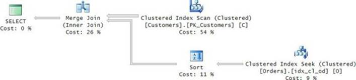
FIGURE 3-22 Plan with a sort operator and merge algorithm.
Observe the small cost percent associated with the sort operation.
Note that such a plan is sensitive to inaccuracies in the cardinality estimate of the activity leading to the Sort operator. That’s especially the case when the estimate is for a small number of rows but the actual is a large number, because sorting doesn’t scale well. For one, a more accurate estimate could lead the optimizer to use a different join algorithm altogether. For two, the low estimate could result in an insufficient memory grant for the sort activity, and this could result in spills to tempdb. You need to be attentive to such problems and, if you spot one, try to figure out ways to help the optimizer come up with a more accurate estimate.
Hash
The hash algorithm involves the creation of a hash table based on one of the inputs—usually the smaller. The reason that the small side is preferred as the build input is that the memory footprint is usually smaller this way. If the hash table fits in memory, it’s ideal. If not, the hash table can be partitioned, but the swapping of partitions in and out of memory makes the algorithm less efficient. The items from the build input are arranged in hash buckets based on the chosen hash function. For illustration purposes, suppose that the join column is an integer one and the optimizer chooses a modulo 50 function as the hash function. Up to 50 hash buckets will be created, with all items that got the same result from the hash function organized in a linked list in the same bucket. Then the other input (known as the probe input) is probed, the hash function is applied to the join column values, and based on the result, the algorithm scans the respective hash bucket to look for matches.
The hash algorithm excels in data-warehouse queries, which tend to involve large amounts of data in the fact table and much smaller dimension tables. It tends to scale well with such queries, benefiting greatly from parallelized processing. Note, though, that the hash table requires a memory grant, and hence this algorithm is sensitive to inaccuracies with cardinality estimates. If there’s an insufficient memory grant, the hash table will spill to tempdb, and this results in less efficient processing.
When using columnstore indexes, the hash algorithm can use batch-execution mode, which is described in Chapter 2. In SQL Server 2012, only inner joins processed with a hash algorithm could use batch execution. Also, if the operator spilled to tempdb, the execution mode switched to row mode. In SQL Server 2014, outer joins processed with a hash algorithm can use batch execution, and so do operators that spill to tempdb.
Besides the classic data warehouse queries, there’s another interesting case where the optimizer tends to choose the hash algorithm—when there aren’t good indexes to support the other algorithms. If you think about it, a hash table is an alternative searching structure to a B-tree. When there are no good existing indexes, it is usually more efficient overall to create a hash table, use it, and drop it in every query execution compared to doing the same thing with a B-tree. As an example, run the following code to drop the two indexes you created earlier to support previous examples:
DROP INDEX idx_nc_cn_i_cid ON dbo.Customers;
DROP INDEX idx_nc_cid_od_i_oid_eid_sid ON dbo.Orders;
Then run the same query you ran earlier in the “Nested loops” section:
SELECT C.custid, C.custname, O.orderid, O.empid, O.shipperid, O.orderdate
FROM dbo.Customers AS C
INNER JOIN dbo.Orders AS O
ON O.custid = C.custid
WHERE C.custname LIKE 'Cust_1000%'
AND O.orderdate >= '20140101'
AND O.orderdate < '20140401';
This time, as a result of the absence of efficient indexes to support a nested loops algorithm, the optimizer chooses to use a hash join with a hash table based on the qualifying customers. The plan for this query is shown in Figure 3-23.
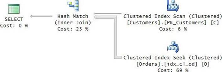
FIGURE 3-23 Plan with a hash algorithm.
So, when you see the optimizer using a hash join in cases where it doesn’t seem natural, ask yourself if you’re missing important indexes—especially if the query is a frequent one in the system.
Forcing join strategy
If you suspect that the optimizer chose a suboptimal join algorithm, you can try a couple of methods for forcing the one you think is more optimal. One is using a join hint where you specify the join algorithm (LOOP, MERGE, or HASH) right before the JOIN keyword, using the full join syntax (INNER <hint> JOIN, LEFT OUTER <hint> JOIN, and so on). Here’s an example for forcing a nested loops algorithm:
SELECT C.custid, C.custname, O.orderid, O.empid, O.shipperid, O.orderdate
FROM dbo.Customers AS C
INNER LOOP JOIN dbo.Orders AS O
ON O.custid = C.custid;
Note that with this method you also force the join order. The left table is used as the outer input, and the right table is used as the inner one.
Another method is to use query hints in the query OPTION clause. The advantage of this method is that you can specify more than one algorithm. Because there are only three supported algorithms, by listing two you are excluding the third. For example, suppose you want to prevent the optimizer from choosing the merge algorithm but you want to leave it with some flexibility to choose between nested loops and hash. You achieve this like so:
SELECT C.custid, C.custname, O.orderid, O.empid, O.shipperid, O.orderdate
FROM dbo.Customers AS C
INNER JOIN dbo.Orders AS O
ON O.custid = C.custid
OPTION(LOOP JOIN, HASH JOIN);
Note, though, that by using this method, all joins in the query are affected. There is no form of a hint that I know of that allows indicating more than one algorithm for a single join. Also note that, unlike the join hint, the query hints for join algorithms don’t affect join ordering. If you want to force the join order, you need to add the FORCE ORDER query hint.
Remember the usual disclaimer concerning performance hints. Such hints are handy as a performance troubleshooting tool; however, using them in production queries removes the dynamic nature of optimization that can normally react to changing circumstances by changing optimization choices. If you do find yourself using such hints in production code to solve critical burning problems, you should consider them a temporary solution. When you have the time, you can more thoroughly research the problem and find a fix that will help the optimizer naturally make more optimal choices.
Separating elements
Separating elements is a classic T-SQL challenge. It involves a table called Arrays with strings holding comma-separated lists of values in a column called arr. Run the following code to create the Arrays table, and populate it with sample data:
SET NOCOUNT ON;
USE tempdb;
IF OBJECT_ID(N'dbo.Arrays', N'U') IS NOT NULL DROP TABLE dbo.Arrays;
CREATE TABLE dbo.Arrays
(
id VARCHAR(10) NOT NULL PRIMARY KEY,
arr VARCHAR(8000) NOT NULL
);
GO
INSERT INTO dbo.Arrays VALUES('A', '20,223,2544,25567,14');
INSERT INTO dbo.Arrays VALUES('B', '30,-23433,28');
INSERT INTO dbo.Arrays VALUES('C', '12,10,8099,12,1200,13,12,14,10,9');
INSERT INTO dbo.Arrays VALUES('D', '-4,-6,-45678,-2');
The challenge is to come up with an efficient solution in T-SQL that splits each string into the individual elements, returned in separate rows along with the id, the position, and the element itself. The desired result looks like the following.
id pos element
---- ---- --------
A 1 20
A 2 223
A 3 2544
A 4 25567
A 5 14
B 1 30
B 2 -23433
B 3 28
...
Note that this task can be solved using .NET more efficiently than with T-SQL—either by using the System.String.Split method or by implementing your own iterative solution. However, our challenge is to implement an efficient solution using T-SQL.
One intuitive approach is to implement an iterative solution as a table function operating on a single string and a separator as inputs and returning a table variable. The function would extract one element in each iteration and insert it into the result table variable. The problem with this approach is that iterative solutions in T-SQL tend to be inefficient.
The challenge, therefore, is to find an efficient set-based solution using T-SQL. To implement such a solution, you will want to split the task into three steps:
1. Generate copies.
2. Extract an element.
3. Calculate the position.
The first step is to generate copies from the original rows—as many as the number of elements in the string. The second step is to extract the relevant element from each copy. The third step is to compute the ordinal position of the element within the string.
For the first step, you will find the auxiliary table Nums from the TSQLV3 database very handy. This table has a column called n that holds a sequence of integers starting with 1. You can think of the numbers as representing character positions in the string. Namely, n = 1 represents character position 1, n = 2 represents character position 2, and so on. To generate copies, you join Arrays and Nums. As the join predicate, use the following expression, which says that the nth character is a comma: SUBSTRING(arr, n, 1) = ‘,’. To avoid extracting a character beyond the end of the string, limit the numbers to the length of the string with the predicate n <= LEN(arr). Here’s the code implementing this logic:
SELECT id, arr, n
FROM dbo.Arrays
INNER JOIN TSQLV3.dbo.Nums
ON n <= LEN(arr)
AND SUBSTRING(arr, n, 1) = ',';
This code generates the following output:
id arr n
----- --------------------- ----
A 20,223,2544,25567,14 3
A 20,223,2544,25567,14 7
A 20,223,2544,25567,14 12
A 20,223,2544,25567,14 18
B 30,-23433,28 3
B 30,-23433,28 10
...
Observe that the output is missing one copy for each string. The reason is that, for a string with X elements, there are X – 1 separators. If you think of the separators as preceding the elements, what’s missing is the separator before the first element. To fix this problem, simply plant a separator at the beginning of the string and pass the result as the first input to the SUBSTRING function. Also, make sure you increase the limit of the number of characters you extract by one to account for the extra character. After these two modifications, the query looks like this:
SELECT id, arr, n
FROM dbo.Arrays
INNER JOIN TSQLV3.dbo.Nums
ON n <= LEN(arr) + 1
AND SUBSTRING(',' + arr, n, 1) = ',';
This query generates the following output:
id arr n
---- --------------------- ----
A 20,223,2544,25567,14 1
A 20,223,2544,25567,14 4
A 20,223,2544,25567,14 8
A 20,223,2544,25567,14 13
A 20,223,2544,25567,14 19
B 30,-23433,28 1
B 30,-23433,28 4
B 30,-23433,28 11
...
This time, you get the right number of copies. In addition, observe that the modifications to the query had an interesting side effect; the character positions where a separator was found increased by one because the whole string shifted one character to the right. This side effect is actually convenient for us because with respect to the original string (without the separator at the beginning), n actually already represents the starting position of the element. So the first step in the solution for the task is accomplished.
The second step is to extract the element that the current copy represents. For this, you will use the SUBSTRING function. You need to pass the string, the starting position, and the length to extract as inputs. You know that the element starts at position n. For the length, you will need to find the position of the next separator and subtract n from it. You can use the CHARINDEX function for this purpose. The first two inputs are the separator you’re looking for and the string where you are looking for it. As the third input, specify n as the starting position to look for the separator. You get the following: CHARINDEX(‘,’, arr, n). The tricky thing here is that there’s no separator after the last element; in such a case, the function returns a 0. To fix this problem, plant a separator at the end of the string, like so: CHARINDEX(‘,’, arr + ‘,’, n). The complete expression extracting the element then becomes: SUBSTRING(arr, n, CHARINDEX(‘,’, arr + ‘,’, n) – n).
The third and last step in the solution is to compute the ordinal position of the element in the string. For this purpose, use the ROW_NUMBER function, partitioned by id and ordered by n.
Here’s the complete solution query:
SELECT id,
ROW_NUMBER() OVER(PARTITION BY id ORDER BY n) AS pos,
SUBSTRING(arr, n, CHARINDEX(',', arr + ',', n) - n) AS element
FROM dbo.Arrays
INNER JOIN TSQLV3.dbo.Nums
ON n <= LEN(arr) + 1
AND SUBSTRING(',' + arr, n, 1) = ',';
If you need to deal with individual input strings, you can encapsulate this logic in an inline table function, like so:
CREATE FUNCTION dbo.Split(@arr AS VARCHAR(8000), @sep AS CHAR(1)) RETURNS TABLE
AS
RETURN
SELECT
ROW_NUMBER() OVER(ORDER BY n) AS pos,
SUBSTRING(@arr, n, CHARINDEX(@sep, @arr + @sep, n) - n) AS element
FROM TSQLV3.dbo.Nums
WHERE n <= LEN(@arr) + 1
AND SUBSTRING(@sep + @arr, n, 1) = @sep;
GO
It’s the same logic, only it operates on a single string instead of a whole table of strings.
As an example, suppose you have a string holding a comma-separated list of order IDs. To split those into a table of elements, use the Split function, like so:
SELECT * FROM dbo.Split('10248,10249,10250', ',') AS S;
You get the following output:
pos element
---- --------
1 10248
2 10249
3 10250
To return further information about the orders in the input string, join the table returned by the function with the Orders table like so:
SELECT O.orderid, O.orderdate, O.custid, O.empid
FROM dbo.Split('10248,10249,10250', ',') AS S
INNER JOIN TSQLV3.Sales.Orders AS O
ON O.orderid = S.element
ORDER BY S.pos;
Observe that the query orders the rows by the ordinal position of the element in the input string. This query generates the following output:
orderid orderdate custid empid
----------- ---------- ----------- -----------
10248 2013-07-04 85 5
10249 2013-07-05 79 6
10250 2013-07-08 34 4
There’s an excellent set of papers written by SQL Server MVP Erland Sommarskog covering the topic of arrays and lists in great depth. You can find those papers here: http://www.sommarskog.se/arrays-in-sql.html.
The UNION, EXCEPT, and INTERSECT operators
The UNION, EXCEPT, and INTERSECT operators are relational operators that combine rows from the result sets of two queries. The general form of code using these operators is shown here:
<query 1>
<operator>
<query 2>
[ORDER BY <order_by_list>];
The UNION operator unifies the rows from the two inputs. The INTERSECT operator returns only the rows that are common to both inputs. The EXCEPT operator returns the rows that appear in the first input but not the second.
The input queries are not allowed to have an ORDER BY clause because they are supposed to return a relational result. However, an ORDER BY clause is allowed against the result of the operator.
The schemas of the input queries need to be compatible. The number of columns has to be the same, and the types need to be implicitly convertible from the one with the lower data type precedence to the higher. The names of the result columns are defined by the first query.
When comparing rows between the inputs, these operators implicitly use the standard distinct predicate. Based on this predicate, one NULL is not distinct from another NULL, and a NULL is distinct from a non-NULL value. Conversely, based on the equality operator, comparing two NULLs results in the logical value unknown, and the same applies when comparing a NULL with a non-NULL value. This fact makes these operators simple and intuitive to use, even when NULLs are possible in the data.
When multiple operators are used in a query without parentheses, INTERSECT precedes UNION and EXCEPT. The last two have the same precedence, so they are evaluated based on appearance order. You can always force your desired evaluation order using parentheses.
The following sections provide more details about these operators.
The UNION ALL and UNION operators
The UNION operator unifies the rows from the two inputs. Figure 3-24 illustrates graphically what the operator does. It shows the result of the operator with a darker background.
FIGURE 3-24 The UNION operator.
T-SQL supports two variations of the UNION operator: UNION (implied DISTINCT) and UNION ALL. Both unify the rows from the two inputs, but only the former removes duplicates from the result; the latter doesn’t. Standard SQL actually supports the explicit form UNION DISTINCT for the former, but T-SQL supports only the implied form.
As an example for UNION, the following code returns distinct unified employee and customer locations:
USE TSQLV3;
SELECT country, region, city FROM HR.Employees
UNION
SELECT country, region, city FROM Sales.Customers;
This query returns 71 distinct locations.
If you want to keep duplicates, use the UNION ALL variation, like so:
SELECT country, region, city FROM HR.Employees
UNION ALL
SELECT country, region, city FROM Sales.Customers;
This query returns 100 rows because it unifies 9 employee rows with 91 customer rows. Usually, it’s not meaningful to return a result with duplicates, but it could be that you need to apply some further logic against the result. For instance, suppose you need to count how many employees plus customers there are in each location. For this, you define a table expression based on the code with the UNION ALL operator and apply the grouping and aggregation in the outer query.
In terms of performance, UNION is usually more expensive than UNION ALL because it involves an extra step that removes duplicates. Figure 3-25 shows the plans for the last UNION and UNION ALL queries demonstrating this.
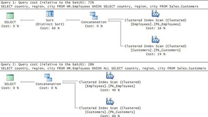
FIGURE 3-25 UNION versus UNION ALL.
The plan for the UNION query uses a Sort (Distinct Sort) operator to remove duplicates. Another option is to use a hash-based algorithm for this purpose. Either way, you can see that there’s more work involved than with the UNION ALL query.
When you unify disjoint inputs, such as data for different years that includes a date column, UNION and UNION ALL become logically equivalent. Unfortunately, many use the UNION operator in such a case because the code involves fewer keystrokes, not realizing the unnecessary extra work taking place. So it’s important to use the UNION ALL operator as your default and reserve the UNION operator only for cases where the result can have duplicates and you need to remove them.
Interestingly, if you use UNION to unify rows from tables and those tables have CHECK constraints defining disjoint intervals, the optimizer can detect this and help you avoid the extra work of removing duplicates. As an example, the following code creates separate tables to store data for different years, with CHECK constraints enforcing the disjoint year intervals:
USE tempdb;
IF OBJECT_ID(N'dbo.T2014', N'U') IS NOT NULL DROP TABLE dbo.T2014;
IF OBJECT_ID(N'dbo.T2015', N'U') IS NOT NULL DROP TABLE dbo.T2015;
GO
CREATE TABLE dbo.T2014
(
keycol INT NOT NULL CONSTRAINT PK_T2014 PRIMARY KEY,
dt DATE NOT NULL CONSTRAINT CHK_T2014_dt CHECK(dt >= '20140101' AND dt < '20150101')
);
CREATE TABLE dbo.T2015
(
keycol INT NOT NULL CONSTRAINT PK_T2015 PRIMARY KEY,
dt DATE NOT NULL CONSTRAINT CHK_T2015_dt CHECK(dt >= '20150101' AND dt < '20160101')
);
Ignoring best practices, you use the following code to unify the rows from the tables with the UNION operator:
SELECT keycol, dt FROM dbo.T2014
UNION
SELECT keycol, dt FROM dbo.T2015;
Fortunately, thanks to the existence of the constraints, the optimizer figures that duplicates cannot exist in the result and therefore optimizes this query the same as it would UNION ALL. The plan for this query is shown in Figure 3-26.
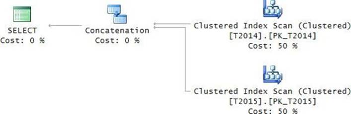
FIGURE 3-26 UNION and CHECK constraints.
It’s still recommended to follow the best practice and stick with UNION ALL as your default for the sake of cases where the optimizer won’t figure out that the inputs are disjoint.
When you’re done testing, run the following code for cleanup:
IF OBJECT_ID(N'dbo.T2014', N'U') IS NOT NULL DROP TABLE dbo.T2014;
IF OBJECT_ID(N'dbo.T2015', N'U') IS NOT NULL DROP TABLE dbo.T2015;
The INTERSECT operator
The INTERSECT operator returns only distinct rows that are common to both inputs. Figure 3-27 illustrates graphically what this operator returns.
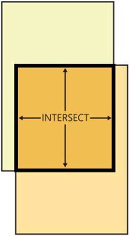
FIGURE 3-27 The INTERSECT operator.
As an example, the following query returns locations that are both employee locations and customer locations:
USE TSQLV3;
SELECT country, region, city FROM HR.Employees
INTERSECT
SELECT country, region, city FROM Sales.Customers;
This query generates the following output:
country region city
--------------- --------------- ---------------
UK NULL London
USA WA Kirkland
USA WA Seattle
Observe in the output that the row with UK, NULL, London was returned because there are both employees and customers in this location. Because the operator uses the distinct predicate implicitly to compare rows, when comparing the NULLs on both sides, it got true and not unknown. If you want to implement the intersection operation with an inner join, you need to add special logic for NULL treatment (with Employees aliased as E and Customers as C):
E.region = C.region OR E.region IS NULL AND C.region IS NULL
Like the UNION operator, INTERSECT returns distinct rows. If a row appears at least once in each of the inputs, it’s returned once in the output. Interestingly, standard SQL supports an operator called INTERSECT ALL, which returns as many occurrences of a row in the result as the minimum number of occurrences between the two inputs. Say that a row R appears X times in the first input and Y times in the second input, the INTERSECT ALL operator returns the row MIN(X, Y) times in the output. It’s as if the operator looks for a separate match for each row. So if you have four occurrences of R in one input and six in the other, you will get R four times in the output.
T-SQL doesn’t support the standard INTERSECT ALL operator, but it’s quite easy to implement your own solution. You achieve this by adding row numbers to both input queries, marking duplicate numbers. You apply the supported INTERSECT operator to the queries with the row numbers. You then define a CTE based on the intersection code, and then in the outer query return the attributes without the row numbers. Here’s the complete solution code:
WITH INTERSECT_ALL
AS
(
SELECT
ROW_NUMBER()
OVER(PARTITION BY country, region, city
ORDER BY (SELECT 0)) AS rn,
country, region, city
FROM HR.Employees
INTERSECT
SELECT
ROW_NUMBER()
OVER(PARTITION BY country, region, city
ORDER BY (SELECT 0)) AS rn,
country, region, city
FROM Sales.Customers
)
SELECT country, region, city
FROM INTERSECT_ALL;
This code generates the following output:
country region city
--------------- --------------- ---------------
UK NULL London
USA WA Kirkland
USA WA Seattle
UK NULL London
UK NULL London
UK NULL London
There are four employees from UK, NULL, London and six customers; doing one-to-one matching, four of them intersect. Therefore, the result has four occurrences of the row.
The EXCEPT operator
The EXCEPT operator returns only distinct rows that appear in the first input but not the second. Figure 3-28 illustrates graphically what this operator returns.
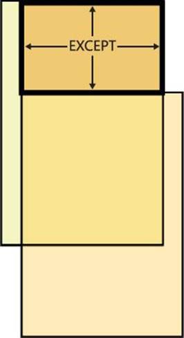
FIGURE 3-28 The EXCEPT operator.
As an example, the following code returns distinct employee locations that are not customer locations:
SELECT country, region, city FROM HR.Employees
EXCEPT
SELECT country, region, city FROM Sales.Customers;
This query generates the following output:
country region city
--------------- --------------- ---------------
USA WA Redmond
USA WA Tacoma
In terms of optimization, like with NOT EXISTS, also with EXCEPT the optimizer can detect that the logical operation is an anti semi join. You can see this if you examine the execution plan for this query.
As it does with INTERSECT ALL, standard SQL supports an operator called EXCEPT ALL, which wasn’t implemented in T-SQL. If a row R appears X times in the first input and Y times in the second input, and X is greater than Y, the operator returns the row X – Y times in the output. The logic behind this is that it’s as if you’re looking for a match for each of the rows and then return only the nonmatches.
To implement your own solution for EXCEPT ALL, you use the same technique you used for INTERSECT ALL. Namely, compute row numbers, marking duplicate numbers in both input queries, and then use the EXCEPT operator. Only the rows from the first input with row numbers that don’t have matches in the second input will be returned. You then define a CTE based on the code with the EXCEPT operator, and in the outer query you return the attributes without the row numbers. Here’s the complete solution code:
WITH EXCEPT_ALL
AS
(
SELECT
ROW_NUMBER()
OVER(PARTITION BY country, region, city
ORDER BY (SELECT 0)) AS rn,
country, region, city
FROM HR.Employees
EXCEPT
SELECT
ROW_NUMBER()
OVER(PARTITION BY country, region, city
ORDER BY (SELECT 0)) AS rn,
country, region, city
FROM Sales.Customers
)
SELECT country, region, city
FROM EXCEPT_ALL;
This code generates the following output:
country region city
--------------- --------------- ---------------
USA WA Redmond
USA WA Tacoma
USA WA Seattle
USA, NULL, Seattle appears twice in Employees and once in Customers; therefore, it is returned once in the output.
As a tip, recall the discussion about finding an efficient solution for the minimum missing value problem earlier in the section “The EXISTS predicate.” Here’s a much simpler and highly efficient solution for the same task using the EXCEPT operator:
SELECT TOP (1) missingval
FROM (SELECT col1 + 1 AS missingval FROM dbo.T1
EXCEPT
SELECT col1 FROM dbo.T1) AS D
ORDER BY missingval;
As with the previously discussed efficient solutions, here also the optimizer uses a Top operator that short-circuits the scans as soon as the first missing value is found.
Conclusion
This chapter covered a lot of ground discussing different tools you use to combine data from multiple tables. It covered subqueries, table expressions, the powerful APPLY operator, joins, and the relational operators UNION, EXCEPT, and INTERSECT. The chapter described both logical considerations for using these tools as well as how to use them optimally.