T-SQL Querying (2015)
Chapter 4. Grouping, pivoting, and windowing
This chapter focuses on performing data-analysis calculations with T-SQL for various purposes, such as reporting. A data-analysis calculation is one you apply to a set of rows and that returns a single value. For example, aggregate calculations fall into this category.
T-SQL supports numerous features and techniques you can use to perform data-analysis calculations, such as window functions, pivoting and unpivoting, computing custom aggregations, and working with multiple grouping sets. This chapter covers such features and techniques.
Window functions
You use window functions to perform data-analysis calculations elegantly and, in many cases, efficiently. In contrast to group functions, which are applied to groups of rows defined by a grouped query, window functions are applied to windows of rows defined by a windowed query. Where a GROUP BY clause determines groups, an OVER clause determines windows. So think of the window as the set of rows, or the context, for the function to apply to.
The design of window functions is quite profound, enabling you to handle data-analysis calculations in many cases more elegantly and more easily than with other tools. Standard SQL acknowledges the immense power in window functions, providing extensive coverage for those. T-SQL implements a subset of the standard, and I hope Microsoft will continue that investment in the future.
The coverage of window functions in this chapter is organized based on their categories: aggregate, ranking, offset, and statistical. There’s also a section with solutions to gaps and islands problems using window functions.
![]() Note
Note
Some of the windowing features described in this section were introduced in Microsoft SQL Server 2012. So if you are using an earlier version of SQL Server, you won’t be able to run the related code samples. Those features include frame specification for aggregate window functions (ORDER BY and ROWS or RANGE window frame units), offset window functions (FIRST_VALUE, LAST_VALUE, LAG, and LEAD), and statistical window functions (PERCENT_RANK, CUME_DIST, PERCENTILE_CONT, and PERCENTILE_DISC).
Aggregate window functions
Aggregate window functions are the same functions you know as grouped functions (SUM, AVG, and others), only you apply them to a window instead of to a group. To demonstrate aggregate window functions, I’ll use a couple of small tables called OrderValues and EmpOrders, and a large table called Transactions. Run the following code to create the tables and fill them with sample data:
SET NOCOUNT ON;
USE tempdb;
-- OrderValues table
IF OBJECT_ID(N'dbo.OrderValues', N'U') IS NOT NULL DROP TABLE dbo.OrderValues;
SELECT * INTO dbo.OrderValues FROM TSQLV3.Sales.OrderValues;
ALTER TABLE dbo.OrderValues ADD CONSTRAINT PK_OrderValues PRIMARY KEY(orderid);
GO
-- EmpOrders table
IF OBJECT_ID(N'dbo.EmpOrders', N'U') IS NOT NULL DROP TABLE dbo.EmpOrders;
SELECT empid, ISNULL(ordermonth, CAST('19000101' AS DATE)) AS ordermonth, qty, val, numorders
INTO dbo.EmpOrders
FROM TSQLV3.Sales.EmpOrders;
ALTER TABLE dbo.EmpOrders ADD CONSTRAINT PK_EmpOrders PRIMARY KEY(empid, ordermonth);
GO
-- Transactions table
IF OBJECT_ID('dbo.Transactions', 'U') IS NOT NULL DROP TABLE dbo.Transactions;
IF OBJECT_ID('dbo.Accounts', 'U') IS NOT NULL DROP TABLE dbo.Accounts;
CREATE TABLE dbo.Accounts
(
actid INT NOT NULL CONSTRAINT PK_Accounts PRIMARY KEY
);
CREATE TABLE dbo.Transactions
(
actid INT NOT NULL,
tranid INT NOT NULL,
val MONEY NOT NULL,
CONSTRAINT PK_Transactions PRIMARY KEY(actid, tranid)
);
DECLARE
@num_partitions AS INT = 100,
@rows_per_partition AS INT = 20000;
INSERT INTO dbo.Accounts WITH (TABLOCK) (actid)
SELECT NP.n
FROM TSQLV3.dbo.GetNums(1, @num_partitions) AS NP;
INSERT INTO dbo.Transactions WITH (TABLOCK) (actid, tranid, val)
SELECT NP.n, RPP.n,
(ABS(CHECKSUM(NEWID())%2)*2-1) * (1 + ABS(CHECKSUM(NEWID())%5))
FROM TSQLV3.dbo.GetNums(1, @num_partitions) AS NP
CROSS JOIN TSQLV3.dbo.GetNums(1, @rows_per_partition) AS RPP;
The OrderValues table has a row per order with total order values and quantities. The EmpOrders table keeps track of monthly totals per employee. The Transactions table has 2,000,000 rows with bank account transactions (100 accounts, with 20,000 transactions in each).
Limitations of data analysis calculations without window functions
Before delving into the details of window functions, you first should realize the limitations of alternative tools that perform data-analysis calculations. Knowing those limitations is a good way to appreciate the ingenious design of window functions.
Consider the following grouped query:
SELECT custid, SUM(val) AS custtotal
FROM dbo.OrderValues
GROUP BY custid;
Compared to analyzing the detail, the grouped query gives you new insights into the data in the form of aggregates. However, the grouped query also hides the detail. For example, the following attempt to return a detail element in a grouped query fails:
SELECT custid, val, SUM(val) AS custtotal
FROM dbo.OrderValues
GROUP BY custid;
You get the following error:
Msg 8120, Level 16, State 1, Line 70
Column 'dbo.OrderValues.val' is invalid in the select list because it is not contained in either
an aggregate function or the GROUP BY clause.
The reference to the val column in the SELECT list is not allowed because it is not part of the grouping set and not contained in a group aggregate function. But what if you do need to return details and aggregates? For example, suppose you want to query the OrderValues table and return, in addition to the order information, the percent of the current order value out of the grand total and also out of the customer total.
You could achieve this with scalar aggregate subqueries, like so:
SELECT orderid, custid, val,
val / (SELECT SUM(val) FROM dbo.OrderValues) AS pctall,
val / (SELECT SUM(val) FROM dbo.OrderValues AS O2
WHERE O2.custid = O1.custid) AS pctcust
FROM dbo.OrderValues AS O1;
Or, if you want formatted output:
SELECT orderid, custid, val,
CAST(100. *
val / (SELECT SUM(val) FROM dbo.OrderValues)
AS NUMERIC(5, 2)) AS pctall,
CAST(100. *
val / (SELECT SUM(val) FROM dbo.OrderValues AS O2
WHERE O2.custid = O1.custid)
AS NUMERIC(5, 2)) AS pctcust
FROM dbo.OrderValues AS O1
ORDER BY custid;
The problem with this approach is that each subquery gets a fresh view of the data as its starting point. Typically, the desired starting point for the set calculation is the underlying query’s result set after most logical query processing phases (table operators, filters, and others) were applied.
For example, suppose you need to filter only orders placed on or after 2015. To achieve this, you add a filter in the underlying query, like so:
SELECT orderid, custid, val,
CAST(100. *
val / (SELECT SUM(val) FROM dbo.OrderValues)
AS NUMERIC(5, 2)) AS pctall,
CAST(100. *
val / (SELECT SUM(val) FROM dbo.OrderValues AS O2
WHERE O2.custid = O1.custid)
AS NUMERIC(5, 2)) AS pctcust
FROM dbo.OrderValues AS O1
WHERE orderdate >= '20150101'
ORDER BY custid;
This filter affects only the underlying query, not the subqueries. The subqueries still query all years. This code generates the following output:
orderid custid val pctall pctcust
-------- ------- -------- ------- --------
10835 1 845.80 0.07 19.79
10952 1 471.20 0.04 11.03
11011 1 933.50 0.07 21.85
10926 2 514.40 0.04 36.67
10856 3 660.00 0.05 9.40
10864 4 282.00 0.02 2.11
10953 4 4441.25 0.35 33.17
10920 4 390.00 0.03 2.91
11016 4 491.50 0.04 3.67
10924 5 1835.70 0.15 7.36
...
There’s a bug in the code. Observe that the percentages per customer don’t sum up to 100 like they should, and the same applies to the percentages out of the grand total. To have the subqueries operate on the underlying query’s result set, you have to either duplicate code elements or use a table expression.
Window functions were designed with the limitations of grouped queries and subqueries in mind, and that’s just the tip of the iceberg in terms of their capabilities!
Unlike grouped queries, windowed queries don’t hide the detail. A window function’s result is returned in addition to the detail.
Unlike the fresh view of the data exposed to a scalar aggregate in a subquery, an OVER clause exposes the underlying query result as the starting point for the window function. More precisely, in terms of logical query processing, window functions operate on the set of rows exposed to the SELECT phase as input—after the handling of FROM, WHERE, GROUP BY, and HAVING. For this reason, window functions are allowed only in the SELECT and ORDER BY clauses of a query. Using an empty specification in the OVER clause defines a window with the entire underlying query result set. So, SUM(val) OVER() gives you the grand total. Adding a window partition clause like PARTITION BY custid restricts the window to only the rows that have the same customer ID as in the current row. So SUM(val) OVER(PARTITION BY custid) gives you the customer total.
The following query then gives you the detail along with the percent of the current order value out of the grand total as well as out of the customer total:
SELECT orderid, custid, val,
val / SUM(val) OVER() AS pctall,
val / SUM(val) OVER(PARTITION BY custid) AS pctcust
FROM dbo.OrderValues;
Here’s a revised version with formatted percentages:
SELECT orderid, custid, val,
CAST(100. * val / SUM(val) OVER() AS NUMERIC(5, 2)) AS pctall,
CAST(100. * val / SUM(val) OVER(PARTITION BY custid) AS NUMERIC(5, 2)) AS pctcust
FROM dbo.OrderValues
ORDER BY custid;
Add a filter to the query:
SELECT orderid, custid, val,
CAST(100. * val / SUM(val) OVER() AS NUMERIC(5, 2)) AS pctall,
CAST(100. * val / SUM(val) OVER(PARTITION BY custid) AS NUMERIC(5, 2)) AS pctcust
FROM dbo.OrderValues
WHERE orderdate >= '20150101'
ORDER BY custid;
Unlike subqueries, window functions get as their starting point the underlying query result after filtering. Observe the query output:
orderid custid val pctall pctcust
-------- ------- -------- ------- --------
10835 1 845.80 0.19 37.58
10952 1 471.20 0.11 20.94
11011 1 933.50 0.21 41.48
10926 2 514.40 0.12 100.00
10856 3 660.00 0.15 100.00
10864 4 282.00 0.06 5.03
10953 4 4441.25 1.01 79.24
10920 4 390.00 0.09 6.96
11016 4 491.50 0.11 8.77
10924 5 1835.70 0.42 27.18
...
Notice that this time the percentages per customer (pctcust) sum up to 100, and the same goes for the percentages out of the grand total when summing those up in all rows.
Window elements
A window function is conceptually evaluated per row, and the elements in the window specification can implicitly or explicitly relate to the underlying row. Aggregate window functions support a number of elements in their specification, as demonstrated by the following query, which computes a running total quantity per employee and month:
SELECT empid, ordermonth, qty,
SUM(qty) OVER(PARTITION BY empid
ORDER BY ordermonth
ROWS BETWEEN UNBOUNDED PRECEDING
AND CURRENT ROW) AS runqty
FROM dbo.EmpOrders;
The window specification can define a window partition and a window frame. Both elements provide ways to restrict a subset of rows from the underlying query’s result set for the function to operate on. The window partition is defined using a window partition clause (PARTITION BY ...). The window frame is defined using a window order clause (ORDER BY ...) and a window frame clause (ROWS | RANGE ...). The following sections describe these window elements in detail.
Window partition
A window partition is a subset of the underlying query’s result set defined by a window partition clause. The window partition is the subset of rows that have the same values in the window partition elements as in the current row. (Remember, the function is evaluated per row.) For example,PARTITION BY empid restricts the rows to only those that have the same empid value as in the current row. Similarly, PARTITION BY custid restricts the rows to only those that have the same custid value as in the current row. Absent a window partition clause, the underlying query result set is considered one big partition. So, for any given row, OVER() exposes to the function the underlying query’s entire result set. Figure 4-1 illustrates what’s considered the qualifying set of rows for the highlighted row with both an empty OVER clause and one containing a window partition clause. The numbers represent customer IDs.
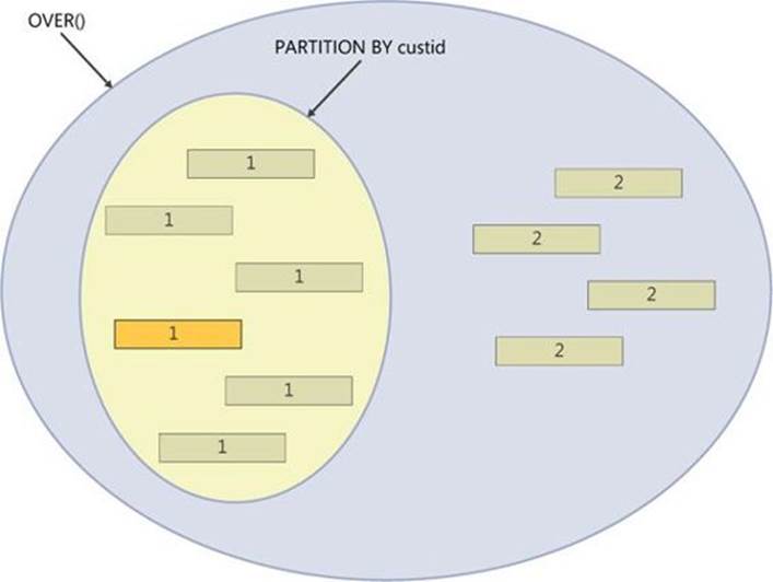
FIGURE 4-1 Window partition.
As an example, the following query computes for each order the percent of the current order value out of the grand total, as well as out of the customer total:
SELECT orderid, custid, val,
CAST(100. * val / SUM(val) OVER() AS NUMERIC(5, 2)) AS pctall,
CAST(100. * val / SUM(val) OVER(PARTITION BY custid) AS NUMERIC(5, 2)) AS pctcust
FROM dbo.OrderValues
ORDER BY custid;
This query generates the following output:
orderid custid val pctall pctcust
-------- ------- ------- ------- --------
10643 1 814.50 0.06 19.06
10692 1 878.00 0.07 20.55
10702 1 330.00 0.03 7.72
10835 1 845.80 0.07 19.79
10952 1 471.20 0.04 11.03
11011 1 933.50 0.07 21.85
10926 2 514.40 0.04 36.67
10759 2 320.00 0.03 22.81
10625 2 479.75 0.04 34.20
10308 2 88.80 0.01 6.33
...
There are clear advantages in terms of simplicity and elegance to using such a windowed query compared to, say, using multiple grouped queries and joining their results. But what about performance? In this respect, I’m afraid the news is not so good. Before I elaborate, I’d like to stress that the inefficiencies I’m about to describe are limited to window aggregate functions without a frame. As I will explain later, window aggregate functions with a frame, window ranking functions, and window offset functions are optimized differently.
To discuss performance aspects, I’ll use the bigger Transactions table, which has 2,000,000 rows. Consider the following query:
SELECT actid, tranid, val,
val / SUM(val) OVER() AS pctall,
val / SUM(val) OVER(PARTITION BY actid) AS pctact
FROM dbo.Transactions;
The execution plan for this query is shown in Figure 4-2.
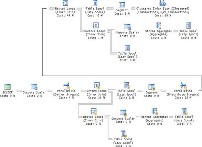
FIGURE 4-2 Optimization with window aggregates.
Recall that the initial set that is exposed to the window function is the underlying query result, after the logical processing phases prior to the SELECT phase have been applied (FROM, WHERE, GROUP BY, and HAVING). Furthermore, the window function’s results are returned in addition to the detail, not instead of it. To ensure both requirements, for each of the window functions, the query plan writes the rows to a spool and then reads from the spool twice—once to compute the aggregate and once to read the detail—and then joins the results. Because the query has two unique window specifications, this work happens twice in the plan.
Clearly, there’s room for improved optimization, especially in cases like ours where there are no table operators, filters, or grouping involved, and there’s an optimal covering index in place (PK_Transactions). Logic can be added to the optimizer to detect cases where there’s no need to spool data, and instead the data is read directly from the index.
With the current optimization resulting in the plan shown in Figure 4-2, on my system, it took the query 13.76 seconds to complete, using 16.485 CPU seconds and 10,053,178 logical reads. That’s a lot for the amount of data involved!
If you rewrite the solution using grouped queries, you will get much better performance. Here’s the version using grouped queries:
WITH GrandAgg AS
(
SELECT SUM(val) AS sumall FROM dbo.Transactions
),
ActAgg AS
(
SELECT actid, SUM(val) AS sumact
FROM dbo.Transactions
GROUP BY actid
)
SELECT T.actid, T.tranid, T.val,
T.val / GA.sumall AS pctall,
T.val / AA.sumact AS pctact
FROM dbo.Transactions AS T
CROSS JOIN GrandAgg AS GA
INNER JOIN ActAgg AS AA
ON AA.actid = T.actid;
Examine the plan shown in Figure 4-3. Observe that there’s no spooling at all, and that efficient order-based aggregates (Stream Aggregate) are computed based on index order.
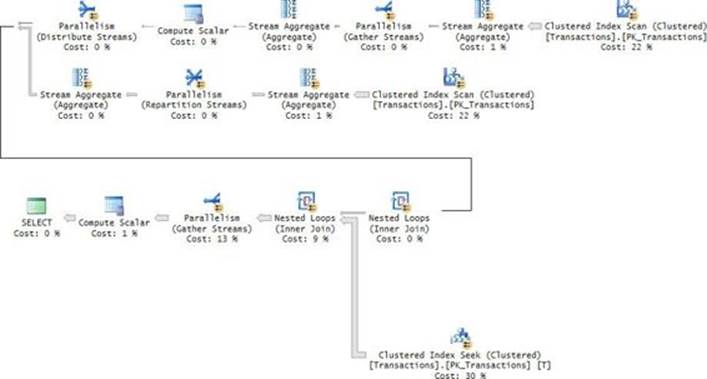
FIGURE 4-3 Optimization with group aggregates.
The performance statistics I got for this solution on my system are as follows:
![]() Run time: 2.01 seconds
Run time: 2.01 seconds
![]() CPU time: 4.97 seconds
CPU time: 4.97 seconds
![]() Logical reads: 19,368
Logical reads: 19,368
That’s quite an improvement.
Because there are great language design benefits in using window functions, we hope to see future investment in better optimization of such functions.
Usually, grouping and windowing are considered different methods to achieve a task, but there are interesting ways to combine them. They are not mutually exclusive. The easiest way to understand this is to think of logical query processing. Remember from Chapter 1, “Logical query processing,” that the GROUP BY clause is evaluated in step 3 and the SELECT clause is evaluated in step 5. Therefore, if the query is a grouped query, the SELECT phase operates on the grouped state of the data and not the detailed state. So if you use a window function in the SELECT or ORDER BY phase, the window function also operates on the grouped state.
As an example, consider the following grouped query:
SELECT custid, SUM(val) AS custtotal
FROM dbo.OrderValues
GROUP BY custid;
The query groups the rows by custid, and it returns the total values per customer (custtotal).
Before looking at the next query, try to answer the following question: Can you add the val column directly to the SELECT list in the preceding query? The answer is, “Of course not.” Because the query is a grouped query, a reference to a column name in the SELECT list is allowed only if the column is part of the GROUP BY list or contained in a group aggregate function.
With this in mind, suppose you need to add to the query a calculation returning the percent of the current customer total out of the grand total. The customer total is expressed with the grouped function SUM(val). Normally, to express the grand total in a detailed query you use a windowed function, SUM(val) OVER(). Now try dividing one by the other, like so:
SELECT custid, SUM(val) AS custtotal,
SUM(val) / SUM(val) OVER() AS pct
FROM dbo.OrderValues
GROUP BY custid;
You get the same error as when trying to add the val column directly to the SELECT list:
Msg 8120, Level 16, State 1, Line 229
Column 'dbo.OrderValues.val' is invalid in the select list because it is not contained in either
an aggregate function or the GROUP BY clause.
Unlike grouped functions, which operate on the detail rows per group, windowed functions operate on the grouped data. Windowed functions can see what the SELECT phase can see. The error message is a bit misleading in that it says “...because it is not contained in either an aggregate function...” and you’re probably thinking that it is. This error message was added to SQL Server well before window functions were introduced. What it means to say is “...because it is not contained in either a group aggregate function....”
If the window function cannot refer to the val column directly, what can it refer to? An attempt to refer to the alias custtotal also fails because of the all-at-once concept in SQL. The answer is that the windowed SUM should be applied to the grouped SUM, like so:
SELECT custid, SUM(val) AS custtotal,
SUM(val) / SUM(SUM(val)) OVER() AS pct
FROM dbo.OrderValues
GROUP BY custid;
This idea takes a bit of getting used to, but when thinking in terms of logical query processing, it makes perfect sense.
Window frame
Just as a partition is a filtered portion of the underlying query’s result set, a frame is a filtered portion of the partition. A frame requires ordering specifications using a window order clause. Based on that order, you define two delimiters that frame the rows. Then the window function is applied to that frame of rows. You can use one of two window frame units: ROWS or RANGE.
I’ll start with ROWS. Using this unit, you can define three types of delimiters:
![]() UNBOUNDED PRECEDING | FOLLOWING: First or last row in the partition, respectively.
UNBOUNDED PRECEDING | FOLLOWING: First or last row in the partition, respectively.
![]() CURRENT ROW: Current row.
CURRENT ROW: Current row.
![]() N ROWS PRECEDING | FOLLOWING: An offset in terms of the specified number of rows (N) before or after the current row, respectively.
N ROWS PRECEDING | FOLLOWING: An offset in terms of the specified number of rows (N) before or after the current row, respectively.
The first delimiter has to be on or before the second delimiter.
Figure 4-4 illustrates the window frame concept. The numbers 1 and 2 represent employee IDs; the values 201307, 201308, and so on represent order months. A sample row is highlighted in bold as the current row.
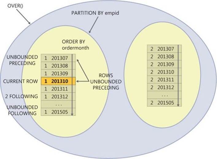
FIGURE 4-4 Window frame.
As an example, suppose you want to query the EmpOrders table and compute for each employee and order month the running total quantity. In other words, you want to see the cumulative performance of the employee over time. You define the window partition clause based on the empidcolumn, the window order clause based on the ordermonth column, and the window frame clause as ROWS BETWEEN UNBOUNDED PRECEDING AND CURRENT ROW, like so:
SELECT empid, ordermonth, qty,
SUM(qty) OVER(PARTITION BY empid
ORDER BY ordermonth
ROWS BETWEEN UNBOUNDED PRECEDING
AND CURRENT ROW) AS runqty
FROM dbo.EmpOrders;
Because this frame specification is so common, the standard defines the equivalent shorter form ROWS UNBOUNDED PRECEDING. Here’s the shorter form used in our query:
SELECT empid, ordermonth, qty,
SUM(qty) OVER(PARTITION BY empid
ORDER BY ordermonth
ROWS UNBOUNDED PRECEDING) AS runqty
FROM dbo.EmpOrders;
This query generates the following output:
empid ordermonth qty runqty
------ ---------- ----- -------
1 2013-07-01 121 121
1 2013-08-01 247 368
1 2013-09-01 255 623
1 2013-10-01 143 766
1 2013-11-01 318 1084
1 2013-12-01 536 1620
...
1 2015-05-01 299 7812
2 2013-07-01 50 50
2 2013-08-01 94 144
2 2013-09-01 137 281
2 2013-10-01 248 529
2 2013-11-01 237 766
2 2013-12-01 319 1085
...
2 2015-04-01 1126 5915
...
Using a window function to compute a running total is both elegant and, as you will soon see, very efficient. An alternative technique is to use a query with a join and grouping, like so:
SELECT O1.empid, O1.ordermonth, O1.qty,
SUM(O2.qty) AS runqty
FROM dbo.EmpOrders AS O1
INNER JOIN dbo.EmpOrders AS O2
ON O2.empid = O1.empid
AND O2.ordermonth <= O1.ordermonth
GROUP BY O1.empid, O1.ordermonth, O1.qty;
This technique is both more complex and gets optimized extremely inefficiently.
To evaluate the optimization of the different techniques, I’ll use the bigger Transactions table. Suppose you need to compute the balance after each transaction for each account. Using a windowed SUM function, you apply the calculation to the val column, partitioned by the actid column, ordered by the tranid column, with the frame ROWS UNBOUNDED PRECEDING.
The optimal index for window functions is what I like to think of as a POC index. This acronym stands for Partitioning (actid, in our case), Ordering (tranid), and Covering (val). The P and O parts should make the index key list, and the C part should be included in the index leaf row. The clustered index PK_Orders on the Transactions table is based on this pattern, so we already have the optimal index in place.
The following query computes the aforementioned bank account balances using a window function:
SELECT actid, tranid, val,
SUM(val) OVER(PARTITION BY actid
ORDER BY tranid
ROWS UNBOUNDED PRECEDING) AS balance
FROM dbo.Transactions;
The plan for this query is shown in Figure 4-5.
![]()
FIGURE 4-5 Plan with fast-track optimization of window function for running totals.
The plan starts by scanning the POC index in order. That’s a good start. The next pair of Segment and Sequence Project operators are responsible for computing row numbers. The row numbers are used to indicate which rows fit in each underlying row’s window frame. The Segment operator flags the next operator when a new partition starts. The Sequence Project operator assigns the row numbers—1 if the row is the first in the partition, and the previous value plus 1 if it is not. The next Segment operator, again, is responsible for flagging the operator to its left when a new partition starts.
Then the next pair of Window Spool and Stream Aggregate operators represent the frame of rows that need to be aggregated and the aggregate applied to the frame, respectively. If it were not for specialized optimization called fast-track that the optimizer employs here, for a partition with N rows, the spool would have to store 1 + 2 + ... + N = (N + N2)/2 rows. As an example, for an account with just 20,000 transactions, the number would be 200,010,000. Fortunately, when the first delimiter of the frame is the first row in the partition (UNBOUNDED PRECEDING), the optimizer detects the case as a “fast-track” case and uses specialized optimization. For each row, it takes the previous row’s accumulation, adds the current row’s value, and writes that to the spool.
With this sort of optimization, you would expect the number of rows going out of the spool to be the same as the number of rows going into it (2,000,000 in our case); however, the plan shows that the number of rows going out of the spool is twice the number going in. The reason for this has to do with the fact that the Stream Aggregate operator was designed well before window functions were introduced. Originally, it was used only to compute group functions in grouped queries, which return the aggregates but hide the detail. So the trick Microsoft used to use the operator to compute a window aggregate is that besides the row with the accumulated aggregate, they also add the detail row to the spool so as not to lose it. So, with fast-track optimization, if N rows go into the Window Spool operator, you should see 2N rows going out.
It took four seconds for the query to complete on my system with results discarded.
Here’s the alternative solution using a join and grouping:
SELECT T1.actid, T1.tranid, T1.val, SUM(T2.val) AS balance
FROM dbo.Transactions AS T1
INNER JOIN dbo.Transactions AS T2
ON T2.actid = T1.actid
AND T2.tranid <= T1.tranid
GROUP BY T1.actid, T1.tranid, T1.val;
Running the query and waiting for it to complete is a good exercise in patience. To understand why, examine the query plan shown in Figure 4-6.
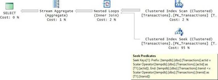
FIGURE 4-6 Plan for running totals with a join and a grouped query.
Here the optimizer doesn’t employ any specialized optimization. You see the POC index scanned once for the T1 instance of the table, and then for each row, it performs a seek in the index representing the instance T2 to the beginning of the current account section, and then a range scan of all rows where T2.actid <= T1.actid. Besides the cost of the full scan of the index and the cost of the seeks, the range scan processes in total (N + N2)/2 rows per account, where N is the number of transactions per account. (In our sample data, N is equal to 20,000.) It took over an hour and a half for the query to finish on my system.
While the plan for the query with the join and grouping has quadratic scaling (N2), the plan for the window function has linear scaling. Furthermore, when the optimizer knows that per underlying row there are no more than 10,000 rows in the window frame, it uses a special optimized in-memory spool (as opposed to a more expensive on-disk spool). Remember that when the unit is ROWS and the optimizer uses fast-track optimization, it writes only two rows to the spool per underlying row—one with the aggregate and one with the detail. In such a case, the conditions for using the in-memory spool are satisfied.
Still, with certain frame specifications like ROWS UNBOUNDED PRECEDING, which are the more commonly used ones, there’s potential for improvements in the optimizer. Theoretically, spooling could be avoided in those cases. Instead, the optimizer could use streaming operators, like the Sequence Project operator it uses to calculate the ROW_NUMBER function. As an example, when replacing the windowed SUM in the query computing balances with the ROW_NUMBER function just to check the performance, the query completes in one second. That’s compared to four seconds for the original query. This is the performance improvement potential for calculations like running totals if Microsoft decides to invest further in this area in the future.
As mentioned, you can use the ROWS option to specify delimiters as an offset in terms of a number of rows before (PRECEDING) or after (FOLLOWING) the current row. As an example, the following query computes for each employee and month the moving average quantity of the last three recorded months.
SELECT empid, ordermonth,
AVG(qty) OVER(PARTITION BY empid
ORDER BY ordermonth
ROWS BETWEEN 2 PRECEDING AND CURRENT ROW) AS avgqty
FROM dbo.EmpOrders;
This query generates the following output:
empid ordermonth avgqty
------ ---------- -------
1 2013-07-01 121
1 2013-08-01 184
1 2013-09-01 207
1 2013-10-01 215
1 2013-11-01 238
1 2013-12-01 332
1 2014-01-01 386
1 2014-02-01 336
1 2014-03-01 249
1 2014-04-01 154
...
As another example, the following query computes the moving average value of the last 100 transactions:
SELECT actid, tranid, val,
AVG(val) OVER(PARTITION BY actid
ORDER BY tranid
ROWS BETWEEN 99 PRECEDING AND CURRENT ROW) AS avg100
FROM dbo.Transactions;
What’s interesting about the optimization of frames that don’t start at the beginning of the partition is that you would expect the optimizer to create a plan that writes all frame rows to the window spool and aggregates them. In the last example, this would mean 100 × 2,000,000 = 2,000,000,000 rows. However, the optimizer has a trick that it can use under certain conditions to avoid such work. If the frame has more than four rows and the aggregate is a cumulative one like SUM, COUNT, or AVG, the optimizer creates a plan with two fast-track running aggregate computations: one starting at the beginning of the partition and ending with the last row in the desired frame (call it CumulativeBottom) and another starting at the beginning of the partition and ending with the row before the start of the desired frame (call it CumulativeTop). Then it derives the final aggregate as a calculation between the two. You can see this strategy employed in the plan for the last query shown in Figure 4-7.
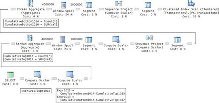
FIGURE 4-7 Plan for moving average.
It took this query 12 seconds to complete on my system. This is not so bad considering the alternative.
If the computation is not cumulative—namely, it cannot be derived from bottom and top calculations—the optimizer will not be able to use any tricks and all applicable rows have to be written to the spool and aggregated. Examples of such aggregates are MIN and MAX. To demonstrate this, the following query uses the MAX aggregate to compute the maximum value among the last 100 transactions:
SELECT actid, tranid, val,
MAX(val) OVER(PARTITION BY actid
ORDER BY tranid
ROWS BETWEEN 99 PRECEDING AND CURRENT ROW) AS max100
FROM dbo.Transactions;
The plan for this query is shown in Figure 4-8.
![]()
FIGURE 4-8 Plan for moving maximum.
Observe the number of rows flowing into and from the Window Spool operator. This query took 64 seconds to complete.
Note that even though the plan chosen is a parallel plan, there’s a trick developed by Adam Machanic you can use that can improve the treatment of parallelism. When the calculation is partitioned (like in our case, where it is partitioned by actid), you can issue a query against the table holding the partitions (Accounts, in our case) and then, with the CROSS APPLY operator, apply a query similar to the original but filtered by the current partition value.
To apply this method to our example, use the following query:
SELECT A.actid, D.tranid, D.val, D.max100
FROM dbo.Accounts AS A
CROSS APPLY (SELECT tranid, val,
MAX(val) OVER(ORDER BY tranid
ROWS BETWEEN 99 PRECEDING AND CURRENT ROW) AS max100
FROM dbo.Transactions AS T
WHERE T.actid = A.actid) AS D;
The plan for this query is shown in Figure 4-9.
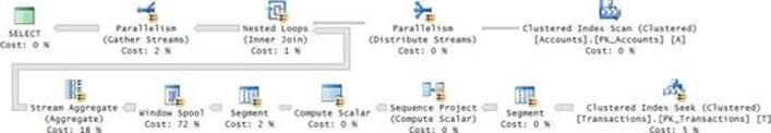
FIGURE 4-9 Optimization with the APPLY operator.
It took this query 30 seconds to complete on my system—half the time of the original query.
Aggregate window functions support another frame unit, called RANGE. Unfortunately though, SQL Server has a limited implementation of this option. In standard SQL, the RANGE option allows you to express the delimiters as an offset from the current row’s ordering value. That’s in contrast to ROWS, which defines the offset in terms of a number of rows. So with RANGE, the definition of the frame is more dynamic.
As an example, suppose you need to compute for each employee and month the moving average quantity of the last three months—not the last three recorded months. The problem is that you don’t have any assurance that every employee had activity in every month. If an employee did not have activity in a certain month, there won’t be a row in the EmpOrders table for that employee in that month. For example, employee 9 had activity in July 2013 and then no activity in August and September, activity in October, no activity in November, and then activity in December. If you use the frame ROWS BETWEEN 2 PRECEDING AND CURRENT ROW to compute the moving average of the last three recorded months, for employee 9 in December 2013 you will capture a period of half a year. The RANGE option is supposed to help you if you need a period of the last three months, never mind how many rows are included. According to standard SQL, you are supposed to use the following query (don’t run it in SQL Server because it’s not supported):
SELECT empid, ordermonth, qty,
SUM(qty) OVER(PARTITION BY empid
ORDER BY ordermonth
RANGE BETWEEN INTERVAL '2' MONTH PRECEDING
AND CURRENT ROW) AS sum3month
FROM dbo.EmpOrders;
As a result, you are supposed to get the following output for employee 9:
empid ordermonth qty sum3month
----------- ---------- ----------- -----------
...
9 2013-07-01 294 294
9 2013-10-01 256 256
9 2013-12-01 25 281
9 2014-01-01 74 99
9 2014-03-01 137 211
9 2014-04-01 52 189
9 2014-05-01 8 197
9 2014-06-01 161 221
9 2014-07-01 4 173
9 2014-08-01 98 263
...
Unfortunately, SQL Server is missing two things to allow such a query. One, SQL Server is missing the INTERVAL feature. Two, SQL Server supports only UNBOUNDED and CURRENT ROW as delimiters for the RANGE unit.
To achieve the task in SQL Server, you have a few options. One is to pad the data with missing employee and month entries, and then use the ROWS option, like so:
DECLARE
@frommonth AS DATE = '20130701',
@tomonth AS DATE = '20150501';
WITH M AS
(
SELECT DATEADD(month, N.n, @frommonth) AS ordermonth
FROM TSQLV3.dbo.GetNums(0, DATEDIFF(month, @frommonth, @tomonth)) AS N
),
R AS
(
SELECT E.empid, M.ordermonth, EO.qty,
SUM(EO.qty) OVER(PARTITION BY E.empid
ORDER BY M.ordermonth
ROWS BETWEEN 2 PRECEDING AND CURRENT ROW) AS sum3month
FROM TSQLV3.HR.Employees AS E CROSS JOIN M
LEFT OUTER JOIN dbo.EmpOrders AS EO
ON E.empid = EO.empid
AND M.ordermonth = EO.ordermonth
)
SELECT empid, ordermonth, qty, sum3month
FROM R
WHERE qty IS NOT NULL;
The other option is to use a query with a join and grouping like the one I showed for the running total example:
SELECT O1.empid, O1.ordermonth, O1.qty,
SUM(O2.qty) AS sum3month
FROM dbo.EmpOrders AS O1
INNER JOIN dbo.EmpOrders AS O2
ON O2.empid = O1.empid
AND O2.ordermonth
BETWEEN DATEADD(month, -2, O1.ordermonth)
AND O1.ordermonth
GROUP BY O1.empid, O1.ordermonth, O1.qty
ORDER BY O1.empid, O1.ordermonth;
The question is, why even bother supporting RANGE with only UNBOUNDED and CURRENT ROW as delimiters? As it turns out, there is a subtle logical difference between ROWS and RANGE when they use the same frame specification. But that difference manifests itself only when the order is not unique. The ROWS option doesn’t include peers (ties in the ordering value), whereas RANGE does. Consider the following query as an example:
SELECT orderid, orderdate, val,
SUM(val) OVER(ORDER BY orderdate ROWS UNBOUNDED PRECEDING) AS sumrows,
SUM(val) OVER(ORDER BY orderdate RANGE UNBOUNDED PRECEDING) AS sumrange
FROM dbo.OrderValues;
This query generates the following output:
orderid orderdate val sumrows sumrange
-------- ---------- -------- ----------- -----------
10248 2013-07-04 440.00 440.00 440.00
10249 2013-07-05 1863.40 2303.40 2303.40
10250 2013-07-08 1552.60 3856.00 4510.06
10251 2013-07-08 654.06 4510.06 4510.06
10252 2013-07-09 3597.90 8107.96 8107.96
...
11070 2015-05-05 1629.98 1257012.06 1263014.56
11071 2015-05-05 484.50 1257496.56 1263014.56
11072 2015-05-05 5218.00 1262714.56 1263014.56
11073 2015-05-05 300.00 1263014.56 1263014.56
11074 2015-05-06 232.09 1263246.65 1265793.22
11075 2015-05-06 498.10 1263744.75 1265793.22
11076 2015-05-06 792.75 1264537.50 1265793.22
11077 2015-05-06 1255.72 1265793.22 1265793.22
The orderdate column isn’t unique. Observe the difference between the results of the functions in orders 10250 and 10251. Notice that in the case of ROWS peers in the orderdate values were not included, making the calculation nondeterministic. Access order to the rows determines which values are included in the calculation. With RANGE, peers were included, so both rows get the same results.
While the logical difference between the two options is subtle, the performance difference is not subtle at all. For the Window Spool operator, the optimizer can use either a special optimized in-memory spool or an on-disk spool like the one used for temporary tables with all the I/O and latching overhead. The risk with the in-memory spool is memory consumption. If the optimizer knows that per underlying row there can’t be more than 10,000 rows in the frame, it uses the in-memory spool. If it either knows that there could be more or is not certain, it will use the on-disk spool. With ROWS, when the fast-track case is detected you have exactly two rows stored in the spool per underlying row, so you always get the in-memory spool. You have a couple of ways to check what kind of spool was used. One is using an extended event calledwindow_spool_ondisk_warning, which is fired when an on-disk spool is used. The other is through STATISTICS IO. The in-memory spool results in zeros in the I/O counters against the worktable, whereas the on-disk spool shows nonzero values.
As an example, run the following query after turning on STATISTICS IO:
SELECT actid, tranid, val,
SUM(val) OVER(PARTITION BY actid
ORDER BY tranid
ROWS UNBOUNDED PRECEDING) AS balance
FROM dbo.Transactions;
It took this query four seconds to complete on my system. Its plan is similar to the one shown earlier in Figure 4-5. Notice that the I/O statistics reported for the worktable are zeros, telling you that the in-memory spool was used:
Table 'Worktable'. Scan count 0, logical reads 0, physical reads 0, read-ahead reads 0,
lob logical reads 0, lob physical reads 0, lob read-ahead reads 0.
Table 'Transactions'. Scan count 1, logical reads 6208, physical reads 168,
read-ahead reads 6200, lob logical reads 0, lob physical reads 0, lob read-ahead reads 0.
Remember that RANGE includes peers, so when using this option, the optimizer cannot know ahead how many rows will need to be included. So whenever you use RANGE, the optimizer always chooses the on-disk spool. Here’s an example using the RANGE option:
SELECT actid, tranid, val,
SUM(val) OVER(PARTITION BY actid
ORDER BY tranid
RANGE UNBOUNDED PRECEDING) AS balance
FROM dbo.Transactions;
Observe that the I/O statistics against the worktable are quite significant this time, telling you that the on-disk spool was used:
Table 'Worktable'. Scan count 2000100, logical reads 12044701, physical reads 0,
read-ahead reads 0, lob logical reads 0, lob physical reads 0, lob read-ahead reads 0.
Table 'Transactions'. Scan count 1, logical reads 6208, physical reads 0, read-ahead reads 0,
lob logical reads 0, lob physical reads 0, lob read-ahead reads 0.
It took this query 37 seconds to complete on my system. That’s an order of magnitude slower than with the ROWS option.
![]() Important
Important
There are two important things you should make a note of. One is that if you specify a window order clause but do not indicate an explicit frame, the default frame is the much slower RANGE UNBOUNDED PRECEDING. The second point is that when the order is unique, ROWS and RANGE that have the same frame specification return the same results, but still the former will be much faster. Unfortunately, the optimizer doesn’t internally convert the RANGE option to ROWS when the ordering is unique to allow better optimization. So unless you have a nonunique order and need to include peers, make sure you indicate ROWS explicitly; otherwise, you will just pay for the unnecessary work.
A classic data-analysis calculation called year-to-date (YTD) is a variation of a running total calculation. It’s just that you need to reset the calculation at the beginning of each year. To achieve this, you specify the expression representing the year, like YEAR(orderdate), in the window partition clause in addition to any other elements you need there.
For example, suppose you need to query the OrderValues table and return for each order the current order info, plus a YTD calculation of the order values per customer based on order date ordering, including peers. This means that your window partition clause will be based on the elements custid, YEAR(orderdate). The window order clause will be based on orderdate. The window frame unit will be RANGE because you are requested not to break ties but rather include them. So even though the RANGE option is the more expensive one, that’s exactly the special case where you are supposed to use it. Here’s the complete query:
SELECT custid, orderid, orderdate, val,
SUM(val) OVER(PARTITION BY custid, YEAR(orderdate)
ORDER BY orderdate
RANGE UNBOUNDED PRECEDING) AS YTD_val
FROM dbo.OrderValues;
This query generates the following output:
custid orderid orderdate val YTD_val
------- -------- ---------- -------- --------
1 10643 2014-08-25 814.50 814.50
1 10692 2014-10-03 878.00 1692.50
1 10702 2014-10-13 330.00 2022.50
1 10835 2015-01-15 845.80 845.80
1 10952 2015-03-16 471.20 1317.00
1 11011 2015-04-09 933.50 2250.50
...
10 10389 2013-12-20 1832.80 1832.80
10 10410 2014-01-10 802.00 1768.80
10 10411 2014-01-10 966.80 1768.80
10 10431 2014-01-30 1892.25 3661.05
10 10492 2014-04-01 851.20 4512.25
...
Observe that customer 10 placed two orders on January 10, 2014, and that the calculation produces the same YTD values in both rows, as it should.
If you need to return only one row per distinct customer and date, you want to first group the rows by the two, and then apply the windowed SUM function to the grouped SUM function. Now that the combination of partitioning and ordering elements is unique, you should use the ROWS unit. Here’s the complete query:
SELECT custid, orderdate,
SUM(SUM(val)) OVER(PARTITION BY custid, YEAR(orderdate)
ORDER BY orderdate
ROWS UNBOUNDED PRECEDING) AS YTD_val
FROM dbo.OrderValues
GROUP BY custid, orderdate;
This query generates the following output:
custid orderdate YTD_val
------- ---------- --------
1 2014-08-25 814.50
1 2014-10-03 1692.50
1 2014-10-13 2022.50
1 2015-01-15 845.80
1 2015-03-16 1317.00
1 2015-04-09 2250.50
...
10 2013-12-20 1832.80
10 2014-01-10 1768.80
10 2014-01-30 3661.05
10 2014-04-01 4512.25
10 2014-11-14 7630.25
...
Observe that now there’s only one row for each unique customer and date, like in the case of customer 10, on January 10, 2014.
Ranking window functions
Ranking calculations are implemented in T-SQL as window functions. When you rank a value, you don’t rank it alone, but rather with respect to some set of values, based on certain order. The windowing concept lends itself to such calculations. The set is defined by the OVER clause. Absent a window partition clause, you rank the current row’s value against all rows in the underlying query’s result set. With a window partition clause, you rank the row against the rows in the same window partition. A mandatory window order clause defines the order for the ranking.
To demonstrate ranking window functions, I’ll use the following Orders table.
SET NOCOUNT ON;
USE tempdb;
IF OBJECT_ID(N'dbo.Orders', N'U') IS NOT NULL DROP TABLE dbo.Orders;
CREATE TABLE dbo.Orders
(
orderid INT NOT NULL,
orderdate DATE NOT NULL,
empid INT NOT NULL,
custid VARCHAR(5) NOT NULL,
qty INT NOT NULL,
CONSTRAINT PK_Orders PRIMARY KEY (orderid)
);
GO
INSERT INTO dbo.Orders(orderid, orderdate, empid, custid, qty)
VALUES(30001, '20130802', 3, 'B', 10),
(10001, '20131224', 1, 'C', 10),
(10005, '20131224', 1, 'A', 30),
(40001, '20140109', 4, 'A', 40),
(10006, '20140118', 1, 'C', 10),
(20001, '20140212', 2, 'B', 20),
(40005, '20140212', 4, 'A', 10),
(20002, '20140216', 2, 'C', 20),
(30003, '20140418', 3, 'B', 15),
(30004, '20140418', 3, 'B', 20),
(30007, '20140907', 3, 'C', 30);
T-SQL supports four ranking functions, called ROW_NUMBER, RANK, DENSE_RANK, and NTILE. Here’s a query demonstrating all four against the Orders table, without a window partition clause, ordered by the qty column:
SELECT orderid, qty,
ROW_NUMBER() OVER(ORDER BY qty) AS rownum,
RANK() OVER(ORDER BY qty) AS rnk,
DENSE_RANK() OVER(ORDER BY qty) AS densernk,
NTILE(4) OVER(ORDER BY qty) AS ntile4
FROM dbo.Orders;
This query generates the following output:
orderid qty rownum rnk densernk ntile4
-------- ---- ------- ---- --------- -------
10001 10 1 1 1 1
10006 10 2 1 1 1
30001 10 3 1 1 1
40005 10 4 1 1 2
30003 15 5 5 2 2
30004 20 6 6 3 2
20001 20 7 6 3 3
20002 20 8 6 3 3
10005 30 9 9 4 3
30007 30 10 9 4 4
40001 40 11 11 5 4
The ROW_NUMBER function is the most commonly used of the four. It computes unique incrementing integers in the target partition (the entire query result in this example), based on the specified order. When the ordering is not unique within the partition, like in our example, the calculation is nondeterministic. Meaning, if you run the query again, you’re not guaranteed to get repeatable results. For example, observe the three rows with the quantity 20. They got the row numbers 6, 7, and 8. What determines which of the three gets which row number is a matter of data layout, optimization, and actual access order. Those things are not guaranteed to be repeatable.
There are cases where you need to guarantee determinism (repeatable results). For example, row numbers can be used for paging purposes, as I will demonstrate in Chapter 5, “TOP and OFFSET-FETCH.” For each page, you submit a query filtering only a certain range of row numbers. You do not want the same row to end up in two different pages even though the underlying data didn’t change just because in one query it got row number 25 and in the other 26. To force a deterministic calculation of row numbers, add a tiebreaker to the window order clause. In our example, extending it to qty, orderid makes the ordering unique, and therefore the calculation deterministic.
RANK and DENSE_RANK differ from ROW_NUMBER in that they produce the same rank value for rows with the same ordering value (quantity, in our case). The difference between RANK and DENSE_RANK is that the former computes one more than the count of rows with lower ordering values than the current, and the latter computes one more than the count of distinct ordering values that are lower than the current. For example, the rows that got row numbers 6, 7, and 8 all got rank values 6 (1 + 5 rows with quantities lower than 20) and dense rank values 3 (1 + 2 distinct quantities that are lower than 20). As a result, rank values can have gaps between them, as is the case between the ranks 1 and 5, whereas dense rank values cannot.
Finally, the NTILE function assigns tile numbers to the rows in the partition based on the specified number of tiles and ordering. In our case, the requested number of tiles is 4 and the ordering is based on the qty column. So, based on quantity ordering, the first fourth of the rows in the result is assigned with tile number 1, the next with 2, and so on. If the count of rows doesn’t divide evenly by the specified number of tiles, assuming R is the remainder, the first R tiles will get an extra row. In our case, we have 11 rows, resulting in a tile size of 2 and a remainder of 3. So the first three tiles will have three rows instead of two. The NTILE calculation is the least commonly used out of the four ranking calculations. Its main use cases are in statistical analysis of data.
Recall that the optional window partition clause is available to all window functions. Here’s an example of a computation of row numbers, partitioned by custid, and ordered by orderid:
SELECT custid, orderid, qty,
ROW_NUMBER() OVER(PARTITION BY custid ORDER BY orderid) AS rownum
FROM dbo.Orders
ORDER BY custid, orderid;
This query generates the following output, where you can see the row numbers are independent for each customer:
custid orderid qty rownum
------ ----------- ----------- --------------------
A 10005 30 1
A 40001 40 2
A 40005 10 3
B 20001 20 1
B 30001 10 2
B 30003 15 3
B 30004 20 4
C 10001 10 1
C 10006 10 2
C 20002 20 3
C 30007 30 4
The query defines presentation order by custid, orderid. Remember that absent a presentation ORDER BY clause, presentation order is not guaranteed.
From an optimization perspective, like with window aggregate functions, the ideal index for a query with a ranking function like ROW_NUMBER is a POC index. Figure 4-10 has the plan for the query when a POC index does not exist.
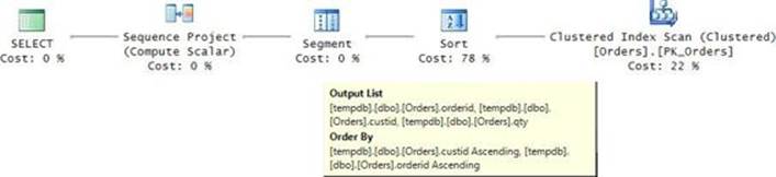
FIGURE 4-10 Optimization of ROW_NUMBER without a POC index.
Because a POC index isn’t present in our case, the optimizer chooses a clustered index scan with an Ordered: False property. It then applies a Sort operator to sort the data by custid, orderid. This order supports both the calculation of the ROW_NUMBER function and the presentation order, which happen to be aligned. The Segment operator flags the Sequence Project operator when a new segment (partition) starts. In turn, the latter returns 1 when the row is the first in the partition, and adds 1 to the previous value when it isn’t.
If you want to avoid the sort, you need to create a POC index, like so:
CREATE UNIQUE INDEX idx_cid_oid_i_qty ON dbo.Orders(custid, orderid) INCLUDE(qty);
Rerun the query, and you get the plan shown in Figure 4-11.
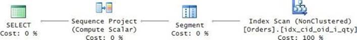
FIGURE 4-11 Optimization of ROW_NUMBER with a POC index.
This time you get an ordered scan of the POC index, and the sort disappears from the plan.
Compared to the previously described optimization of aggregate window functions, ROW_NUMBER, RANK, and DENSE_RANK are optimized using superfast streaming operators; there’s no spooling. It would certainly be great to see in the future similar optimization of aggregate functions that use common specialized frames like ROWS UNBOUNDED PRECEDING.
As for NTILE, the optimizer needs to know the count of rows in the query result in order to compute the tile size. For this, it uses optimization similar to adding the window aggregate COUNT(*) OVER(), with the spooling technique demonstrated earlier in Figure 4-2.
There’s a curious thing about the ROW_NUMBER function and window ordering. A window order clause is mandatory, and it cannot be a constant; though there’s no requirement for the window ordering to be unique. These requirements impose a challenge when you want to compute row numbers just for uniqueness purposes and you don’t care about order. You also don’t want to pay any unnecessary costs that are related to arranging the data in the required order. If you attempt to omit the window order clause, you get an error. If you try to specify a constant likeORDER BY NULL, you get an error. Surprisingly, SQL Server is happy when you provide a subquery returning a constant, as in ORDER BY (SELECT NULL). Here’s an example for a query using this trick:
SELECT orderid, orderdate, custid, empid, qty,
ROW_NUMBER() OVER(ORDER BY (SELECT NULL)) AS rownum
FROM dbo.Orders;
The optimizer realizes that because all rows will have the same ordering value, it doesn’t really need the data in any order. So it assigns the row numbers simply based on access order (data layout, optimization).
Offset window functions
You use offset window functions to request an element from a row that is at the beginning or end of the window frame or is in a certain offset from the current row. I’ll first describe a pair of offset window functions called FIRST_VALUE and LAST_VALUE, and then I’ll describe the pair LAG and LEAD.
FIRST_VALUE and LAST_VALUE
You can use the FIRST_VALUE and LAST_VALUE functions to return an element from the first or last row in the window frame, respectively. The frame specification is the same as what I described in the “Window frame” section in the “Aggregate window functions” topic. This includes the discussion about the critical performance difference between ROWS and RANGE.
You will usually use the FIRST_VALUE and LAST_VALUE functions when you need to return something from the first or last row in the partition. In such a case, you will want to use FIRST_VALUE with the frame ROWS BETWEEN UNBOUNDED PRECEDING AND CURRENT ROW, and LAST_VALUE with the frame ROWS BETWEEN CURRENT ROW AND UNBOUNDED FOLLOWING.
As an example, the following query against the Orders table returns with each order the quantity of the same customer’s first order (firstqty) and last order (lastqty):
SELECT custid, orderid, orderdate, qty,
FIRST_VALUE(qty) OVER(PARTITION BY custid
ORDER BY orderdate, orderid
ROWS BETWEEN UNBOUNDED PRECEDING
AND CURRENT ROW) AS firstqty,
LAST_VALUE(qty) OVER(PARTITION BY custid
ORDER BY orderdate, orderid
ROWS BETWEEN CURRENT ROW
AND UNBOUNDED FOLLOWING) AS lastqty
FROM dbo.Orders
ORDER BY custid, orderdate, orderid;
This query generates the following output:
custid orderid orderdate qty firstqty lastqty
------ ----------- ---------- ----------- ----------- -----------
A 10005 2013-12-24 30 30 10
A 40001 2014-01-09 40 30 10
A 40005 2014-02-12 10 30 10
B 30001 2013-08-02 10 10 20
B 20001 2014-02-12 20 10 20
B 30003 2014-04-18 15 10 20
B 30004 2014-04-18 20 10 20
C 10001 2013-12-24 10 10 30
C 10006 2014-01-18 10 10 30
C 20002 2014-02-16 20 10 30
C 30007 2014-09-07 30 10 30
Typically, you will use these functions combined with other elements in the calculation. For example, compute the difference between the current order quantity and the quantity of the same customer’s first order, as in qty – FIRST_VALUE(qty) OVER(...).
As with all window functions, the window partition clause is optional. As you could probably guess, the window order clause is mandatory. An explicit window frame specification is optional, but recall that once you have a window order clause, there is a frame; and the default frame isRANGE UNBOUNDED PRECEDING. So you want to make sure you specify the frame explicitly; otherwise, you will have problems with both functions. With the FIRST_VALUE function, the default frame will give you the element from the first row in the partition. However, remember that the default RANGE option is much more expensive than ROWS. As for LAST_VALUE, the last row in the default frame is the current row, and not the last row in the partition.
As for optimization, the FIRST_VALUE and LAST_VALUE functions are optimized like aggregate window functions with the same frame specification.
LAG and LEAD
You can use the LAG and LEAD functions to return an element from the previous or next row, respectively. As you might have guessed, a window order clause is mandatory with these functions. Typical uses for these functions include trend analysis (the difference between the current and previous months’ values), recency (the difference between the current and previous orders’ supply dates), and so on.
As an example, the following query returns along with order information the quantities of the same customer’s previous and next orders:
SELECT custid, orderid, orderdate, qty,
LAG(qty) OVER(PARTITION BY custid
ORDER BY orderdate, orderid) AS prevqty,
LEAD(qty) OVER(PARTITION BY custid
ORDER BY orderdate, orderid) AS nextqty
FROM dbo.Orders
ORDER BY custid, orderdate, orderid;
This query generates the following output:
custid orderid orderdate qty prevqty nextqty
------ ----------- ---------- ----------- ----------- -----------
A 10005 2013-12-24 30 NULL 40
A 40001 2014-01-09 40 30 10
A 40005 2014-02-12 10 40 NULL
B 30001 2013-08-02 10 NULL 20
B 20001 2014-02-12 20 10 15
B 30003 2014-04-18 15 20 20
B 30004 2014-04-18 20 15 NULL
C 10001 2013-12-24 10 NULL 10
C 10006 2014-01-18 10 10 20
C 20002 2014-02-16 20 10 30
C 30007 2014-09-07 30 20 NULL
As you can see, the LAG function returns a NULL for the first row in the partition and the LEAD function returns a NULL for the last.
These functions support a second parameter indicating the offset in case you want it to be other than NULL, and a third parameter indicating the default instead of a NULL in case a row doesn’t exist in the requested offset. For example, the expression LAG(qty, 3, 0) returns the quantity from three rows before the current row and 0 if a row doesn’t exist in that offset.
As for optimization, the LAG and LEAD functions are internally converted to the LAST_VALUE function with a frame made of one row. In the case of LAG, the frame used is ROWS BETWEEN 1 PRECEDING AND 1 PRECEDING; in the case of LEAD, the frame is ROWS BETWEEN 1 FOLLOWING AND 1 FOLLOWING.
Statistical window functions
T-SQL supports two pairs of statistical window functions that provide information about distribution of data. One pair of functions provides rank distribution information and another provides inverse distribution information.
Rank distribution functions
Rank distribution functions give you the relative rank of a row expressed as a percent (in the range 0 through 1) in the target partition based on the specified order. T-SQL supports two such functions, called PERCENT_RANK and CUME_DIST. Each of the two computes the rank a bit differently.
Following are the elements involved in the formulas for the two computations:
![]() rk = Rank of the row based on the same specification as the distribution function.
rk = Rank of the row based on the same specification as the distribution function.
![]() nr = Count of rows in the partition.
nr = Count of rows in the partition.
![]() np = Number of rows that precede or are peers of the current row.
np = Number of rows that precede or are peers of the current row.
The formula used to compute PERCENT_RANK is (rk – 1) / (nr – 1).
The formula used to compute CUME_DIST is np / nr.
As an example, the following query uses these functions to compute rank distribution information of student test scores:
USE TSQLV3;
SELECT testid, studentid, score,
CAST( 100.00 *
PERCENT_RANK() OVER(PARTITION BY testid ORDER BY score)
AS NUMERIC(5, 2) ) AS percentrank,
CAST( 100.00 *
CUME_DIST() OVER(PARTITION BY testid ORDER BY score)
AS NUMERIC(5, 2) ) AS cumedist
FROM Stats.Scores;
This query generates the following output:
testid studentid score percentrank cumedist
---------- ---------- ----- ------------ ---------
Test ABC Student E 50 0.00 11.11
Test ABC Student C 55 12.50 33.33
Test ABC Student D 55 12.50 33.33
Test ABC Student H 65 37.50 44.44
Test ABC Student I 75 50.00 55.56
Test ABC Student B 80 62.50 77.78
Test ABC Student F 80 62.50 77.78
Test ABC Student A 95 87.50 100.00
Test ABC Student G 95 87.50 100.00
Test XYZ Student E 50 0.00 10.00
Test XYZ Student C 55 11.11 30.00
Test XYZ Student D 55 11.11 30.00
Test XYZ Student H 65 33.33 40.00
Test XYZ Student I 75 44.44 50.00
Test XYZ Student B 80 55.56 70.00
Test XYZ Student F 80 55.56 70.00
Test XYZ Student A 95 77.78 100.00
Test XYZ Student G 95 77.78 100.00
Test XYZ Student J 95 77.78 100.00
Inverse distribution functions
Inverse distribution functions compute percentiles. A percentile N is the value below which N percent of the observations fall. For example, the 50th percentile (aka median) test score is the score below which 50 percent of the scores fall.
There are two distribution models that can be used to compute percentiles: discrete and continuous. When the requested percentile exists as an exact value in the population, both models return that value. For example, when computing the median with an odd number of elements, both models result in the middle element. The two models differ when the requested percentile doesn’t exist as an actual value in the population. For example, when computing the median with an even number of elements, there is no middle point. In such a case, the discrete model returns the element closest to the missing one. In the median’s case, you get the value just before the missing one. The continuous model interpolates the missing value from the two surrounding it, assuming continuous distribution. In the median’s case, it’s the average of the two middle values.
T-SQL provides two window functions, called PERCENTILE_DISC and PERCENTILE_CONT, that implement the discrete and continuous models, respectively. You specify the percentile you’re after as an input value in the range 0 to 1. Using a clause called WITHIN GROUP, you specify the order. As is usual with window functions, you can apply the calculation against the entire query result set or against a restricted partition using a window partition clause.
As an example, the following query computes the median student test scores within the same test using both models:
SELECT testid, studentid, score,
PERCENTILE_DISC(0.5) WITHIN GROUP(ORDER BY score)
OVER(PARTITION BY testid) AS mediandisc,
PERCENTILE_CONT(0.5) WITHIN GROUP(ORDER BY score)
OVER(PARTITION BY testid) AS mediancont
FROM Stats.Scores;
Because a window function is not supposed to hide the detail, you get the results along with the detail rows. The same results get repeated for all rows in the same partition. Here’s the output of this query:
testid studentid score mediandisc mediancont
---------- ---------- ----- ---------- ----------------------
Test ABC Student E 50 75 75
Test ABC Student C 55 75 75
Test ABC Student D 55 75 75
Test ABC Student H 65 75 75
Test ABC Student I 75 75 75
Test ABC Student B 80 75 75
Test ABC Student F 80 75 75
Test ABC Student A 95 75 75
Test ABC Student G 95 75 75
Test XYZ Student E 50 75 77.5
Test XYZ Student C 55 75 77.5
Test XYZ Student D 55 75 77.5
Test XYZ Student H 65 75 77.5
Test XYZ Student I 75 75 77.5
Test XYZ Student B 80 75 77.5
Test XYZ Student F 80 75 77.5
Test XYZ Student A 95 75 77.5
Test XYZ Student G 95 75 77.5
Test XYZ Student J 95 75 77.5
Observe that for Test ABC the two functions return the same results because there’s an odd number of rows. For Test XYZ, the results are different because there’s an even number of elements. Remember that in the case of median, when there’s an even number of elements the two models use different calculations.
Standard SQL supports inverse distribution functions as grouped ordered set functions. That’s convenient when you need to return the percentile calculation once per group (test, in our case) and not repeated with all detail rows. Unfortunately, ordered set functions are not supported yet in SQL Server. But just to give you a sense, here’s how you would compute the median in both models per test (don’t try running this in SQL Server):
SELECT testid,
PERCENTILE_DISC(0.5) WITHIN GROUP(ORDER BY score) AS mediandisc,
PERCENTILE_CONT(0.5) WITHIN GROUP(ORDER BY score) AS mediancont
FROM Stats.Scores
GROUP BY testid;
![]() Note
Note
You can find a SQL Server feature enhancement request about ordered set functions here: https://connect.microsoft.com/SQLServer/feedback/details/728969. We hope we will see this feature implemented in the future. The concept is applicable not just to inverse-distribution functions but to any set function that has ordering relevance.
The alternative in SQL Server is to use the window functions and eliminate duplicates with a DISTINCT clause, like so:
SELECT DISTINCT testid,
PERCENTILE_DISC(0.5) WITHIN GROUP(ORDER BY score)
OVER(PARTITION BY testid) AS mediandisc,
PERCENTILE_CONT(0.5) WITHIN GROUP(ORDER BY score)
OVER(PARTITION BY testid) AS mediancont
FROM Stats.Scores;
This query generates the following output:
testid mediandisc mediancont
---------- ---------- ----------------------
Test ABC 75 75
Test XYZ 75 77.5
From an optimization perspective, these functions are optimized very inefficiently. The query plan has a number of rounds where the rows are spooled, and then the spool is read once to compute an aggregate and once for the detail. See Chapter 5 for a discussion about more efficient alternatives.
Gaps and islands
Gaps and islands are classic problems in T-SQL that involve a sequence of values. The type of the values is usually date and time, but sometimes integer and others. The gaps task involves identifying the ranges of missing values, and the islands task involves identifying the ranges of existing values. Examples for gaps and islands tasks are identifying periods of inactivity and periods of activity, respectively. Many gaps and islands tasks can be solved efficiently using window functions.
I’ll first demonstrate solutions using a sequence of integers simply because it’s much easier to explain the logic with integers. In reality, most gaps and islands tasks involve date and time sequences. Once you figure out a technique to solve the task using a sequence of integers, you need to perform fairly minor adjustments to apply it to a date-and-time sequence.
For sample data, I’ll use the following table T1:
SET NOCOUNT ON;
USE tempdb;
IF OBJECT_ID('dbo.T1', 'U') IS NOT NULL DROP TABLE dbo.T1;
CREATE TABLE dbo.T1(col1 INT NOT NULL CONSTRAINT PK_T1 PRIMARY KEY);
GO
INSERT INTO dbo.T1(col1) VALUES(1),(2),(3),(7),(8),(9),(11),(15),(16),(17),(28);
Gaps
The gaps task is about identifying the ranges of missing values in the sequence as intervals. I’ll demonstrate a technique to handle the task against the table T1.
One of the simplest and most efficient techniques involves two steps. The first is to return for each current col1 value (call it cur) the immediate next value using the LEAD function (call it nxt). This is achieved with the following query:
SELECT col1 AS cur, LEAD(col1) OVER(ORDER BY col1) AS nxt
FROM dbo.T1;
This query generates the following output:
cur nxt
----------- -----------
1 2
2 3
3 7
7 8
8 9
9 11
11 15
15 16
16 17
17 28
28 NULL
We have an index on col1, so the plan for this query does a single ordered scan of the index to support the LEAD calculation.
Examine the pairs of cur-nxt values, and observe that the pairs where the difference is greater than one represent gaps. The second step involves defining a CTE based on the last query, and then filtering the pairs representing gaps, adding one to cur and subtracting one from nxt to return the actual gap information. Here’s the complete solution query:
WITH C AS
(
SELECT col1 AS cur, LEAD(col1) OVER(ORDER BY col1) AS nxt
FROM dbo.T1
)
SELECT cur + 1 AS range_from, nxt - 1 AS range_to
FROM C
WHERE nxt - cur > 1;
This query generates the following output:
range_from range_to
----------- -----------
4 6
10 10
12 14
18 27
Notice also that the pair with the NULL in nxt was naturally filtered out because the difference was NULL, NULL > 1 is unknown, and unknown gets filtered out.
Islands
The islands task is the inverse of the gaps task. Identifying islands means returning the ranges of consecutive values. I’ll first demonstrate a solution using the generic sequence of integers in T1.col1, and then I’ll use a more realistic example using a sequence of dates.
One of the most beautiful and efficient techniques to identify islands involves computing row numbers based on the order of the sequence column, and using those to compute an island identifier. To see how this can be achieved, first compute row numbers based on col1 order, like so:
SELECT col1, ROW_NUMBER() OVER(ORDER BY col1) AS rownum
FROM dbo.T1;
This query generates the following output:
col1 rownum
----------- --------------------
1 1
2 2
3 3
7 4
8 5
9 6
11 7
15 8
16 9
17 10
28 11
Look carefully at the two sequences and see if you can identify an interesting relationship between them that can help you identify islands. For this, focus your attention on one of the islands. If you do enough staring at the output, you will figure it out at some point—within an island, both sequences keep incrementing by a fixed interval of 1 integer; therefore, the difference between the two is the same within the island. Also, when switching from one island to the next rownum increases by 1, whereas col1 increases by more than 1; therefore, the difference keeps growing from one island to the next and hence is unique per island. This means you can use the difference as the island, or group, identifier. Run the following query to compute the group identifier (grp) based on this logic:
SELECT col1, col1 - ROW_NUMBER() OVER(ORDER BY col1) AS grp
FROM dbo.T1;
This query generates the following output:
col1 grp
----------- --------------------
1 0
2 0
3 0
7 3
8 3
9 3
11 4
15 7
16 7
17 7
28 17
Because there’s an index defined on col1, the computation of the row numbers doesn’t require explicit sorting, as can be seen in the plan for this query in Figure 4-12.

FIGURE 4-12 Plan for query computing group identifier.
Most of the cost of this plan is in the ordered scan of the index PK_T1. The rest of the work involving the calculation of the row numbers and the computation of the difference between the sequences is negligible.
Finally, you need to define a CTE based on the last query, and then in the outer query group the rows by grp, return the minimum col1 value as the start of the island, and return the maximum as the end. Here’s the complete solution query:
WITH C AS
(
SELECT col1, col1 - ROW_NUMBER() OVER(ORDER BY col1) AS grp
FROM dbo.T1
)
SELECT MIN(col1) AS range_from, MAX(col1) AS range_to
FROM C
GROUP BY grp;
This query generates the following output:
range_from range_to
----------- -----------
1 3
7 9
11 11
15 17
28 28
The col1 sequence in T1 has unique values, but you should be aware that if duplicate values were possible, the solution would not work correctly anymore. That’s because the ROW_NUMBER function generates unique values in the target partition, even for rows with the same ordering values. For the logic to be correct, you need a ranking function that assigns the same ranking values for all rows with the same ordering values, with no gaps between distinct ranking values. Fortunately, such a ranking function exists—that’s the DENSE_RANK function. Here’s the revised solution using DENSE_RANK:
WITH C AS
(
SELECT col1, col1 - DENSE_RANK() OVER(ORDER BY col1) AS grp
FROM dbo.T1
)
SELECT MIN(col1) AS range_from, MAX(col1) AS range_to
FROM C
GROUP BY grp;
Because the DENSE_RANK function works correctly both when the sequence is unique and when it isn’t, it makes sense to always use DENSE_RANK and not ROW_NUMBER. It’s just easier to explain the logic first with a unique sequence using the ROW_NUMBER function, and then examine a nonunique sequence, and then explain why DENSE_RANK is preferred.
As mentioned, in most cases in reality you will need to identify islands involving date and time sequences. As an example, suppose you need to query the Sales.Orders table in the TSQLV3 database, and identify for each shipper the islands of shipped date values. The shipped date values are stored in the shippeddate column. Clearly you can have duplicate values in this column. Also, not all orders recorded in the table are shipped orders; those that were not yet shipped have a NULL shipped date. For the purpose of identifying islands, you should simply ignore those NULLs. To support your solution, you need an index on the partitioning column shipperid, sequence column shippeddate, and tiebreaker column orderid as the keys. Because NULLs are possible and should be ignored, you add a filter that excludes NULLs from the index definition. Run the following code to create the recommended index:
USE TSQLV3;
CREATE UNIQUE INDEX idx_sid_sd_oid
ON Sales.Orders(shipperid, shippeddate, orderid)
WHERE shippeddate IS NOT NULL;
When computing the group identifier for the islands in col1 in T1, both the col1 values and the dense rank values were integers with the same interval 1. With the shippeddate sequence, things are trickier because the shipped date values and the dense rank values are of different types; one is temporal and the other is integer. Still, the interval between consecutive values in each is fixed, only in one case it’s the temporal interval 1 day and in the other it’s the integer interval 1. So, to apply the logic in this case, you subtract from the temporal shipped date value the dense rank value times the temporal interval (1 day). This way, the group identifier will be a temporal value, but like before it will be the same for all members of the same island.
Here’s the complete solution query implementing this logic:
WITH C AS
(
SELECT shipperid, shippeddate,
DATEADD(
day,
-1 * DENSE_RANK() OVER(PARTITION BY shipperid ORDER BY shippeddate),
shippeddate) AS grp
FROM Sales.Orders
WHERE shippeddate IS NOT NULL
)
SELECT shipperid,
MIN(shippeddate) AS fromdate,
MAX(shippeddate) AS todate,
COUNT(*) as numorders
FROM C
GROUP BY shipperid, grp;
A good way to understand the logic behind computing the group identifier is to first run the inner query, which defines the CTE C, and examine the result. You will get the following output:
shipperid shippeddate grp
----------- ----------- ----------
1 2013-07-10 2013-07-09
1 2013-07-15 2013-07-13
1 2013-07-23 2013-07-20
1 2013-07-29 2013-07-25
1 2013-08-02 2013-07-28
1 2013-08-06 2013-07-31
1 2013-08-09 2013-08-02
1 2013-08-09 2013-08-02
...
1 2014-01-10 2013-12-07
1 2014-01-13 2013-12-09
1 2014-01-14 2013-12-09
1 2014-01-14 2013-12-09
1 2014-01-22 2013-12-16
...
You will notice that the dates that belong to the same island get the same group identifier.
The plan for the inner query defining the CTE C can be seen in Figure 4-13.

FIGURE 4-13 Plan for inner query computing group identifier with dates.
This plan is very efficient. It performs an ordered scan of the index you prepared for this solution to support the computation of the dense rank values. The cost of the rest of the work in the plan is negligible.
The complete solution generates the ranges of shipped date values as the following output shows:
shipperid fromdate todate numorders
----------- ---------- ---------- -----------
1 2013-07-10 2013-07-10 1
2 2013-07-11 2013-07-12 2
1 2013-07-15 2013-07-15 1
2 2013-07-16 2013-07-17 2
3 2013-07-15 2013-07-16 2
...
There are different variations of islands challenges. A common and interesting one is when you need to identify islands while ignoring gaps of up to a certain size. For example, in our challenge to identify islands of shipped dates per shipper, suppose you need to ignore gaps of up to 7 days.
A very elegant solution to this variation involves the use of two window functions: LAG and SUM. You use LAG to return for each current order the shipped date of the previous order that was shipped by the same shipper. Using a CASE expression, you compute a flag called startflagthat is set to 0 if the difference between the previous and the current dates is less than or equal to 7 and 1 otherwise. Here’s the code implementing this step:
SELECT shipperid, shippeddate, orderid,
CASE WHEN DATEDIFF(day,
LAG(shippeddate) OVER(PARTITION BY shipperid ORDER BY shippeddate, orderid),
shippeddate) <= 7 THEN 0 ELSE 1 END AS startflag
FROM Sales.Orders
WHERE shippeddate IS NOT NULL;
This query generates the following output:
shipperid shippeddate orderid startflag
----------- ----------- ----------- -----------
1 2013-07-10 10249 1
1 2013-07-15 10251 0
1 2013-07-23 10258 1
1 2013-07-29 10260 0
1 2013-08-02 10270 0
1 2013-08-06 10267 0
1 2013-08-09 10269 0
1 2013-08-09 10275 0
1 2013-08-12 10265 0
1 2013-08-16 10274 0
1 2013-08-21 10281 0
1 2013-08-21 10282 0
1 2013-08-27 10284 0
1 2013-09-03 10288 0
1 2013-09-03 10290 0
1 2013-09-11 10296 1
1 2013-09-12 10280 0
...
As you can see, the startflag flag marks the start of each island with a 1 and a nonstart of an island with a 0. Next, using the SUM window aggregate function, you compute the group identifier as the running total of the startflag flag over time, like so:
WITH C1 AS
(
SELECT shipperid, shippeddate, orderid,
CASE WHEN DATEDIFF(day,
LAG(shippeddate) OVER(PARTITION BY shipperid ORDER BY shippeddate, orderid),
shippeddate) <= 7 THEN 0 ELSE 1 END AS startflag
FROM Sales.Orders
WHERE shippeddate IS NOT NULL
)
SELECT *,
SUM(startflag) OVER(PARTITION BY shipperid
ORDER BY shippeddate, orderid
ROWS UNBOUNDED PRECEDING) AS grp
FROM C1;
This query generates the following output:
shipperid shippeddate orderid startflag grp
----------- ----------- ----------- ----------- -----------
1 2013-07-10 10249 1 1
1 2013-07-15 10251 0 1
1 2013-07-23 10258 1 2
1 2013-07-29 10260 0 2
1 2013-08-02 10270 0 2
1 2013-08-06 10267 0 2
1 2013-08-09 10269 0 2
1 2013-08-09 10275 0 2
1 2013-08-12 10265 0 2
1 2013-08-16 10274 0 2
1 2013-08-21 10281 0 2
1 2013-08-21 10282 0 2
1 2013-08-27 10284 0 2
1 2013-09-03 10288 0 2
1 2013-09-03 10290 0 2
1 2013-09-11 10296 1 3
1 2013-09-12 10280 0 3
...
Observe that the group identifier, as required, is the same for all members of the same island and is unique per island. The final step is to group the rows by shipperid and grp, and return the minimum and maximum shipped dates per island, like so:
WITH C1 AS
(
SELECT shipperid, shippeddate, orderid,
CASE WHEN DATEDIFF(day,
LAG(shippeddate) OVER(PARTITION BY shipperid ORDER BY shippeddate, orderid),
shippeddate) <= 7 THEN 0 ELSE 1 END AS startflag
FROM Sales.Orders
WHERE shippeddate IS NOT NULL
),
C2 AS
(
SELECT *,
SUM(startflag) OVER(PARTITION BY shipperid
ORDER BY shippeddate, orderid
ROWS UNBOUNDED PRECEDING) AS grp
FROM C1
)
SELECT shipperid,
MIN(shippeddate) AS fromdate,
MAX(shippeddate) AS todate,
COUNT(*) as numorders
FROM C2
GROUP BY shipperid, grp;
This query generates the following output:
shipperid fromdate todate numorders
----------- ---------- ---------- -----------
2 2014-12-31 2015-05-06 118
3 2013-09-11 2013-09-11 1
2 2013-08-26 2013-11-15 33
1 2014-04-04 2014-05-07 11
3 2013-07-15 2013-08-02 8
3 2013-11-18 2014-01-28 31
1 2013-12-13 2014-01-14 12
3 2014-05-12 2014-05-27 5
1 2014-08-06 2014-12-15 57
2 2014-06-18 2014-07-04 8
3 2013-08-12 2013-08-14 3
...
Examine the query plan for this solution, which is shown in Figure 4-14.
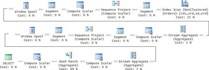
FIGURE 4-14 Plan for query identifying islands ignoring gaps of up to seven days.
Amazingly, not even one sort operation was required throughout the plan. Index order was relied on for the calculation of both the LAG and SUM window functions.
When you’re done, run the following code to drop the index you created for this example:
DROP INDEX idx_sid_sd_oid ON Sales.Orders;
Pivoting
Pivoting is an operation that rotates data from a state of rows to a state of columns. There are different reasons to pivot data. A common reason is related to reporting: you have a certain amount of data to present but a limited space in the web page or printed report. Pivoting helps you fit more data in less space. Also, visually it’s often convenient to analyze data presented as the intersection of dimensions represented by rows and columns. Other reasons to use pivoting are to handle custom aggregates (as I will discuss later in the chapter), solve relational division problems, and more.
There are two kinds of pivot operations: one-to-one and many-to-one. I’ll describe both in the following sections.
One-to-one pivot
In a one-to-one pivot operation, you return in the result the exact same data you had in the source, only using a different shape. Multiple values from the same column in different source rows are returned as different column values of the same result row. This is best explained through a practical example.
As an example for a scenario where you need to apply a one-to-one pivot operation, I’ll use a modeling scheme known as open schema and also as dynamic schema. You have a table called OpenSchema where you keep track of object attribute values using a model known as EAV (for entity, attribute, and value). In this model, you store each object attribute value in a separate row. Each object can have a different set of applicable attributes. Each attribute can be of a different type, so SQL_VARIANT is used as the type for the value column.
Run the following code to create the OpenSchema table and populate it with some sample data:
USE tempdb;
IF OBJECT_ID(N'dbo.OpenSchema', N'U') IS NOT NULL DROP TABLE dbo.OpenSchema;
CREATE TABLE dbo.OpenSchema
(
objectid INT NOT NULL,
attribute NVARCHAR(30) NOT NULL,
value SQL_VARIANT NOT NULL,
CONSTRAINT PK_OpenSchema PRIMARY KEY (objectid, attribute)
);
GO
INSERT INTO dbo.OpenSchema(objectid, attribute, value) VALUES
(1, N'attr1', CAST(CAST('ABC' AS VARCHAR(10)) AS SQL_VARIANT)),
(1, N'attr2', CAST(CAST(10 AS INT) AS SQL_VARIANT)),
(1, N'attr3', CAST(CAST('20130101' AS DATE) AS SQL_VARIANT)),
(2, N'attr2', CAST(CAST(12 AS INT) AS SQL_VARIANT)),
(2, N'attr3', CAST(CAST('20150101' AS DATE) AS SQL_VARIANT)),
(2, N'attr4', CAST(CAST('Y' AS CHAR(1)) AS SQL_VARIANT)),
(2, N'attr5', CAST(CAST(13.7 AS NUMERIC(9,3))AS SQL_VARIANT)),
(3, N'attr1', CAST(CAST('XYZ' AS VARCHAR(10)) AS SQL_VARIANT)),
(3, N'attr2', CAST(CAST(20 AS INT) AS SQL_VARIANT)),
(3, N'attr3', CAST(CAST('20140101' AS DATE) AS SQL_VARIANT));
Run the following query to show the contents of the table:
SELECT objectid, attribute, value FROM dbo.OpenSchema;
This query generates the following output:
objectid attribute value
--------- ---------- ------------------------
1 attr1 ABC
1 attr2 10
1 attr3 2013-01-01 00:00:00.000
2 attr2 12
2 attr3 2015-01-01 00:00:00.000
2 attr4 Y
2 attr5 13.700
3 attr1 XYZ
3 attr2 20
3 attr3 2014-01-01 00:00:00.000
As you can imagine, implementing dynamic schema using the EAV model has advantages and disadvantages compared to alternative models. But that’s not your concern—for reasons that have already been debated, this model was chosen. The problem is that attempting to query the data in its current form can be complex. The values of different attributes for the same object are stored in different rows, so even simple requests can result in complex relational division queries. To make reporting simpler, once a night the data needs to be pivoted and the pivoted form should be persisted in a table. Then reports can be issued off of that table, requiring simpler and more efficient queries.
Your task is to write a query that pivots the data into the following form:
objectid attr1 attr2 attr3 attr4 attr5
----------- ------ ------ ------------------------ ------ -------
1 ABC 10 2013-01-01 00:00:00.000 NULL NULL
2 NULL 12 2015-01-01 00:00:00.000 Y 13.700
3 XYZ 20 2014-01-01 00:00:00.000 NULL NULL
The result of your query should have a row per distinct object ID, a column per distinct attribute, and the applicable value in the intersection of each object ID and attribute.
A pivot operation involves three steps, described here using the open schema example:
1. Grouping by objectid Each set of rows that are associated with the same object are going to be represented by a single result row. You achieve this step by grouping the data. In our example, the grouping column is objectid. In T-SQL, you simply use GROUP BY objectid.
2. Spreading attribute IN (attr1, attr2, attr3, attr4, attr5) The values in the value column should be spread to different result columns based on the attribute that the current row is associated with. The spreading column in our case is the attribute column. You need to identify the distinct elements in the spreading column; those become column names in the result. In our case, the distinct elements are attr1, attr2, attr3, attr4, and attr5. For each such spreading element, you need to write an expression that implements conditional logic to return the value only when it’s applicable. For example, for the element attr1, the logic should be as follows: if the current row is associated with attr1, return the value from the value column; otherwise, return a NULL as a placeholder. To implement this logic in T-SQL, you use the expression CASE WHEN attribute = ‘attr1’ THEN value END. When you don’t indicate an ELSE clause, ELSE NULL is assumed by default. You use such an expression for each distinct spreading element.
3. Aggregating MAX(val) Remember that the query is implemented as a grouped query and each object is going to be represented by a single result row. With one-to-one pivoting per group, each CASE expression will return at most one applicable value; all the rest will be NULLs. The purpose of the third step is to return that applicable value if it exists and to return NULL otherwise. Because the query is a grouped query, the only tool you are allowed to use for this purpose is an aggregate function applied to the result of the CASE expression. With at most one applicable value per group, you could use the function MAX (or MIN). The function ignores NULLs and works with most data types. So the aggregate function in our case is MAX, and it is applied to the results of the CASE expression (the value column when it’s applicable). To summarize, our aggregation element is MAX(val).
The three steps combined give you the following solution query:
SELECT objectid,
MAX(CASE WHEN attribute = 'attr1' THEN value END) AS attr1,
MAX(CASE WHEN attribute = 'attr2' THEN value END) AS attr2,
MAX(CASE WHEN attribute = 'attr3' THEN value END) AS attr3,
MAX(CASE WHEN attribute = 'attr4' THEN value END) AS attr4,
MAX(CASE WHEN attribute = 'attr5' THEN value END) AS attr5
FROM dbo.OpenSchema
GROUP BY objectid;
The execution plan for this query is shown in Figure 4-15.
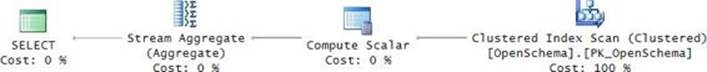
FIGURE 4-15 Plan for a standard pivot query.
The plan looks like a plan for a normal grouped query with the extra Compute Scalar operator handling the CASE expressions. The index PK_OpenSchema is defined based on the key-list (objectid, attribute), so it has the rows in the desired order, and because it’s a clustered index it covers the query. The plan scans the index in order and then provides the rows in that order to the Stream Aggregate operator. As you can see, it’s a very efficient plan.
A question that often comes up is how do you deal with a case where you don’t know ahead of time what the distinct spreading values are? The answer is that you have to query the distinct values from the data, construct a string with the pivot query based on those values, and then use dynamic SQL to execute it. I will demonstrate how this can be done later in the chapter when discussing specialized solutions for custom aggregations.
The preceding technique to pivot data uses only standard SQL constructs, so it’s a very portable technique. Also, as you will see in the section about many-to-one pivoting, you can easily extend it to support multiple aggregates when needed without adding much cost.
T-SQL supports an alternative technique using a proprietary table operator called PIVOT. Like any table operator, you use it in the FROM clause of your query. You use the following syntax:
SELECT <col_list>
FROM <source> PIVOT(<agg_func>(<agg_col>) FOR <spreading_col> IN (<spreading_elements>)) AS P;
Identifying the elements involved in our pivot task, the solution query looks like this:
SELECT objectid, attr1, attr2, attr3, attr4, attr5
FROM dbo.OpenSchema
PIVOT(MAX(value) FOR attribute IN(attr1, attr2, attr3, attr4, attr5)) AS P;
Observe that the spreading elements are specified in this syntax already as identifiers of column names and not the literal character strings they used to be in the source. If the identifier happens to be irregular (starts with a digit, has spaces, is a reserved keyword, and so on), you need to delimit it with double quotes or square brackets, as in “2015”.
The plan for this query is shown in Figure 4-16.
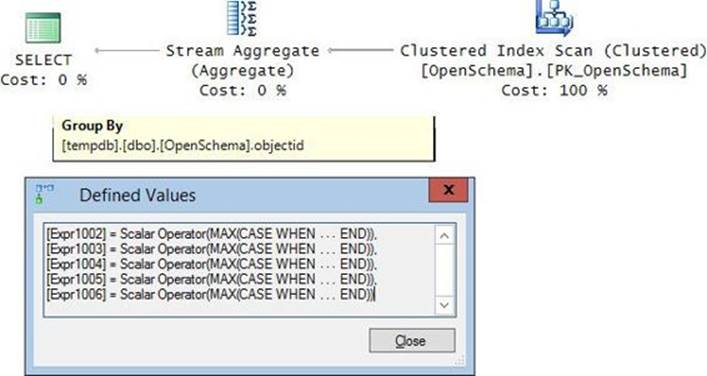
FIGURE 4-16 Plan for a pivot query with the PIVOT operator.
If you look at the properties of the Stream Aggregate operator, you will find a small surprise: SQL Server generated CASE expressions similar to the ones you used in the previous solution. So you realize that from a performance perspective, the two solutions are treated pretty much the same.
A curious thing about the syntax of the PIVOT operator is that while you do indicate the spreading and aggregation parts, you do not indicate the grouping columns. This part is implied; the grouping columns are all columns from the queried table that were not mentioned as the spreading and aggregation columns. In our case, the only column left in the OpenSchema table is objectid. But you realize the danger in this syntax; if you add columns to the table in the future, the next time you run the query those columns implicitly also become part of the grouping. For this reason, it is recommended that instead of querying the table directly as the source for the PIVOT operator, you define a table expression like a derived table or CTE, where you project only the columns that need to play a role in the pivot operation. Here’s an example for implementing this approach using a derived table:
SELECT objectid, attr1, attr2, attr3, attr4, attr5
FROM (SELECT objectid, attribute, value FROM dbo.OpenSchema) AS D
PIVOT(MAX(value) FOR attribute IN(attr1, attr2, attr3, attr4, attr5)) AS P;
This way, your code is safe and you don’t need to be concerned about future additions of columns to the table.
This syntax has the advantage that it is less verbose than the previous solution. However, it has a few disadvantages. It is proprietary, so it is less portable. You are limited to only one aggregate function. It might not be apparent why you would want multiple functions when discussing one-to-one pivoting, but with many-to-one pivoting it could be needed. This syntax doesn’t allow expressions that manipulate the spreading or aggregation columns. Any needed manipulation has to be done in a table expression that you will use as the input for the PIVOT operator.
In case you were wondering, T-SQL doesn’t support providing a subquery as input to the IN clause. Like I explained with the previous solution, if the spreading values are unknown ahead of time, you need to construct the query string yourself and use dynamic SQL to execute it. I will demonstrate an example later in the chapter.
Many-to-one pivot
A many-to-one pivot is a kind of pivot where you can have multiple source rows represented by a single target row-column intersection. Although the aggregate function used in the one-to-one case is artificial, in the many-to-one case it’s meaningful. That’s pretty much the difference. Otherwise, the techniques used in both cases are the same.
As an example, suppose you need to query the Sales.OrderValues view in the TSQLV3 database. You want to pivot data so that you return a row per customer, a column per order year, and in the intersection of each customer and year, you want to return the sum of applicable values. The grouping column in this case is custid. The spreading column is orderyear (the result of the YEAR function applied to the orderdate column), with the distinct spreading elements currently being 2013, 2014, and 2015. The aggregation function is SUM applied to the column val. To allow using the alias orderyear in the computations, you can define it in a table expression.
Here’s the solution query using the standard method with the grouping and CASE expressions:
USE TSQLV3;
SELECT custid,
SUM(CASE WHEN orderyear = 2013 THEN val END) AS [2013],
SUM(CASE WHEN orderyear = 2014 THEN val END) AS [2014],
SUM(CASE WHEN orderyear = 2015 THEN val END) AS [2015]
FROM (SELECT custid, YEAR(orderdate) AS orderyear, val
FROM Sales.OrderValues) AS D
GROUP BY custid;
This query generates the following output:
custid 2013 2014 2015
------- -------- --------- ---------
1 NULL 2022.50 2250.50
2 88.80 799.75 514.40
3 403.20 5960.78 660.00
4 1379.00 6406.90 5604.75
5 4324.40 13849.02 6754.16
6 NULL 1079.80 2160.00
7 9986.20 7817.88 730.00
8 982.00 3026.85 224.00
9 4074.28 11208.36 6680.61
10 1832.80 7630.25 11338.56
...
Here’s the solution query using the PIVOT operator:
SELECT custid, [2013],[2014],[2015]
FROM (SELECT custid, YEAR(orderdate) AS orderyear, val
FROM Sales.OrderValues) AS D
PIVOT(SUM(val) FOR orderyear IN([2013],[2014],[2015])) AS P;
As mentioned, the advantage of the PIVOT operator is in the brevity of the code, and one of its disadvantages is that it’s limited to only one aggregate. So what if you need to support multiple aggregates using the standard solution, and you end up with so many expressions that the length of the code becomes an issue for you? There is a method that can help you shorten the query string.
You create a helper table called Matrix with a row and a column per distinct spreading value. You fill the table with 1s only when the row and column represent the same spreading value. Here’s the code to create and populate the Matrix table to support our pivot task, followed by a query that presents its contents:
IF OBJECT_ID(N'dbo.Matrix', N'U') IS NOT NULL DROP TABLE dbo.Matrix;
CREATE TABLE dbo.Matrix
(
orderyear INT NOT NULL PRIMARY KEY,
y2013 INT NULL,
y2014 INT NULL,
y2015 INT NULL
);
GO
INSERT INTO dbo.Matrix(orderyear, y2013) VALUES(2013, 1);
INSERT INTO dbo.Matrix(orderyear, y2014) VALUES(2014, 1);
INSERT INTO dbo.Matrix(orderyear, y2015) VALUES(2015, 1);
SELECT orderyear, y2013, y2014, y2015 FROM dbo.Matrix;
The query generates the following output:
orderyear y2013 y2014 y2015
----------- ----------- ----------- -----------
2013 1 NULL NULL
2014 NULL 1 NULL
2015 NULL NULL 1
Then to shorten the standard solution’s length, you do the following:
![]() Join the source table (D in our case) with the Matrix table, matching rows based on an equality between the orderyear values on both sides.
Join the source table (D in our case) with the Matrix table, matching rows based on an equality between the orderyear values on both sides.
![]() Instead of the CASE expression form of SUM(CASE WHEN orderyear = 2015 THEN val END), use SUM(val*y2015). The two are equivalent because in both cases, when the year is 2015 the value in the val column is returned (y2015 is 1), and when the year is different a NULL is returned.
Instead of the CASE expression form of SUM(CASE WHEN orderyear = 2015 THEN val END), use SUM(val*y2015). The two are equivalent because in both cases, when the year is 2015 the value in the val column is returned (y2015 is 1), and when the year is different a NULL is returned.
Here’s the complete solution query:
SELECT custid,
SUM(val*y2013) AS [2013],
SUM(val*y2014) AS [2014],
SUM(val*y2015) AS [2015]
FROM (SELECT custid, YEAR(orderdate) AS orderyear, val
FROM Sales.OrderValues) AS D
INNER JOIN dbo.Matrix AS M ON D.orderyear = M.orderyear
GROUP BY custid;
If you want to compute a count instead of a sum, without the Matrix table you either replace the SUM function with COUNT or use the following trick:
SELECT custid,
SUM(CASE WHEN orderyear = 2013 THEN 1 END) AS [2013],
SUM(CASE WHEN orderyear = 2014 THEN 1 END) AS [2014],
SUM(CASE WHEN orderyear = 2015 THEN 1 END) AS [2015]
FROM (SELECT custid, YEAR(orderdate) AS orderyear
FROM Sales.Orders) AS D
GROUP BY custid;
You return a 1 for each applicable order, and therefore the sum of applicable 1s gives you the count. This query generates the following output:
custid 2013 2014 2015
------- ----- ----- -----
1 NULL 3 3
2 1 2 1
3 1 5 1
4 2 7 4
5 3 10 5
6 NULL 4 3
7 3 7 1
8 1 1 1
9 3 8 6
10 1 5 8
...
Using the Matrix table, you just apply the SUM function directly to the Matrix column, like so:
SELECT custid,
SUM(y2013) AS [2013],
SUM(y2014) AS [2014],
SUM(y2015) AS [2015]
FROM (SELECT custid, YEAR(orderdate) AS orderyear
FROM Sales.Orders) AS D
INNER JOIN dbo.Matrix AS M ON D.orderyear = M.orderyear
GROUP BY custid;
Because the Matrix column has a 1 only when the order was placed in that year, the SUM function computes a count in practice.
Remember one of the benefits in using the standard method was the fact that it can support multiple aggregate functions without adding significant cost. Here’s an example computing the sum, average, and count:
SELECT custid,
SUM(val*y2013) AS sum2013,
SUM(val*y2014) AS sum2014,
SUM(val*y2015) AS sum2015,
AVG(val*y2013) AS avg2013,
AVG(val*y2014) AS avg2014,
AVG(val*y2015) AS avg2015,
SUM(y2013) AS cnt2013,
SUM(y2014) AS cnt2014,
SUM(y2015) AS cnt2015
FROM (SELECT custid, YEAR(orderdate) AS orderyear, val
FROM Sales.OrderValues) AS D
INNER JOIN dbo.Matrix AS M ON D.orderyear = M.orderyear
GROUP BY custid;
Recall the motivation for using the technique with the Matrix table was to shorten the query string. The benefit might not be apparent when you have a small number of expressions, but imagine if you had dozens or hundreds; then the benefit is realized.
Unpivoting
Unpivoting is an operation that rotates data from a state of columns to rows. The starting point for an unpivot task is source data stored in pivoted form. As an example, use the following code to create the table PvtOrders, fill it with sample data, and then query it to present its contents:
IF OBJECT_ID(N'dbo.PvtOrders', N'U') IS NOT NULL DROP TABLE dbo.PvtOrders;
SELECT custid, [2013], [2014], [2015]
INTO dbo.PvtOrders
FROM (SELECT custid, YEAR(orderdate) AS orderyear, val
FROM Sales.OrderValues) AS D
PIVOT(SUM(val) FOR orderyear IN([2013],[2014],[2015])) AS P;
SELECT custid, [2013], [2014], [2015] FROM dbo.PvtOrders;
The query generates the following output:
custid 2013 2014 2015
------- -------- --------- ---------
1 NULL 2022.50 2250.50
2 88.80 799.75 514.40
3 403.20 5960.78 660.00
4 1379.00 6406.90 5604.75
5 4324.40 13849.02 6754.16
6 NULL 1079.80 2160.00
7 9986.20 7817.88 730.00
8 982.00 3026.85 224.00
9 4074.28 11208.36 6680.61
10 1832.80 7630.25 11338.56
...
It’s common for data to be stored like this in spreadsheets. Imagine you just imported the data from a spreadsheet to the database. It’s not very convenient to query the data in its current shape, so you want to unpivot it to a form that has a row per customer and year. In the following sections, I will describe a number of methods to achieve this unpivot task.
Unpivoting with CROSS JOIN and VALUES
You can split an unpivot task into three steps:
1. Generate copies.
2. Extract the element.
3. Remove NULLs.
I will describe these steps applied to our example.
The first step is about generating copies from the source rows. You need as many copies as the number of columns that you need to unpivot. In our case, the columns you need to unpivot represent order years, so you need a copy per order year. You can use the VALUES clause to define a derived table called Y holding order years, like so:
(VALUES(2013),(2014),(2015)) AS Y(orderyear)
Here’s a query against the derived table presenting its contents:
SELECT orderyear FROM (VALUES(2013),(2014),(2015)) AS Y(orderyear);
This query generates the following output:
orderyear
-----------
2013
2014
2015
To generate copies, you perform a cross join between the source table PvtOrders and the table Y holding the order years, like so:
SELECT custid, [2013], [2014], [2015], orderyear
FROM dbo.PvtOrders
CROSS JOIN (VALUES(2013),(2014),(2015)) AS Y(orderyear);
This query generates the following output:
custid 2013 2014 2015 orderyear
------- ------- -------- -------- ----------
1 NULL 2022.50 2250.50 2013
1 NULL 2022.50 2250.50 2014
1 NULL 2022.50 2250.50 2015
2 88.80 799.75 514.40 2013
2 88.80 799.75 514.40 2014
2 88.80 799.75 514.40 2015
3 403.20 5960.78 660.00 2013
3 403.20 5960.78 660.00 2014
3 403.20 5960.78 660.00 2015
...
The second step is about extracting the value from the right column in each copy to generate the result val column. What determines which column’s value to return is the value in the orderyear column. When it’s 2013, you need to return the value from the column [2013]; when it’s 2014, you need to return the value from the column [2014], and so on. To implement this step, you can use a simple CASE expression, like so:
SELECT custid, orderyear,
CASE orderyear
WHEN 2013 THEN [2013]
WHEN 2014 THEN [2014]
WHEN 2015 THEN [2015]
END AS val
FROM dbo.PvtOrders
CROSS JOIN (VALUES(2013),(2014),(2015)) AS Y(orderyear);
This query generates the following output:
custid orderyear val
----------- ----------- --------
1 2013 NULL
1 2014 2022.50
1 2015 2250.50
2 2013 88.80
2 2014 799.75
2 2015 514.40
3 2013 403.20
3 2014 5960.78
3 2015 660.00
...
Finally, the third step is supposed to remove the rows that are inapplicable (representing no activity). Those are the ones with a NULL in the val column. You cannot refer to the val column alias in the WHERE clause because it’s defined in the SELECT list. As a workaround, you can define the alias in a VALUES clause using the CROSS APPLY operator, and then refer to it in the query’s WHERE clause, like so:
SELECT custid, orderyear, val
FROM dbo.PvtOrders
CROSS JOIN (VALUES(2013),(2014),(2015)) AS Y(orderyear)
CROSS APPLY (VALUES(CASE orderyear
WHEN 2013 THEN [2013]
WHEN 2014 THEN [2014]
WHEN 2015 THEN [2015]
END)) AS A(val)
WHERE val IS NOT NULL;
This query generates the following output where the rows with a NULL in the val column are removed:
custid orderyear val
----------- ----------- ---------------------------------------
1 2014 2022.50
1 2015 2250.50
2 2013 88.80
2 2014 799.75
2 2015 514.40
3 2013 403.20
3 2014 5960.78
3 2015 660.00
...
Unpivoting with CROSS APPLY and VALUES
There’s a more elegant way to achieve unpivoting compared to the previous method. You combine the steps that generate the copies and extract the element into one step by using CROSS APPLY and VALUES. The CROSS APPLY operator gives the right table expression visibility to the elements of the left row. The right table expression can use the VALUES clause to produce multiple rows out of each left row. Each row is formed from a constant for the result orderyear column, and the corresponding column value for the result val column.
Here’s the solution query:
SELECT custid, orderyear, val
FROM dbo.PvtOrders
CROSS APPLY (VALUES(2013, [2013]),(2014, [2014]),(2015, [2015])) AS A(orderyear, val)
WHERE val IS NOT NULL;
What’s interesting about this technique is that it can be used in more complex unpivoting tasks. To demonstrate such a task, I’ll use a table called Sales that you create and populate by running the following code:
USE tempdb;
IF OBJECT_ID(N'dbo.Sales', N'U') IS NOT NULL DROP TABLE dbo.Sales;
GO
CREATE TABLE dbo.Sales
(
custid VARCHAR(10) NOT NULL,
qty2013 INT NULL,
qty2014 INT NULL,
qty2015 INT NULL,
val2013 MONEY NULL,
val2014 MONEY NULL,
val2015 MONEY NULL,
CONSTRAINT PK_Sales PRIMARY KEY(custid)
);
INSERT INTO dbo.Sales
(custid, qty2013, qty2014, qty2015, val2013, val2014, val2015)
VALUES
('A', 606,113,781,4632.00,6877.00,4815.00),
('B', 243,861,637,2125.00,8413.00,4476.00),
('C', 932,117,202,9068.00,342.00,9083.00),
('D', 915,833,138,1131.00,9923.00,4164.00),
('E', 822,246,870,1907.00,3860.00,7399.00);
Here you need to unpivot not just one, but two sets of columns; one with quantities in different order years, and another with values. To achieve this, you use a solution similar to the last one, only each row in the VALUES clause is formed from three elements: the constant for the order year, the column holding the quantity for that year, and the column holding the value for that year. Here’s the complete solution query:
SELECT custid, salesyear, qty, val
FROM dbo.Sales
CROSS APPLY
(VALUES(2013, qty2013, val2013),
(2014, qty2014, val2014),
(2015, qty2015, val2015)) AS A(salesyear, qty, val)
WHERE qty IS NOT NULL OR val IS NOT NULL;
This query generates the following output:
custid salesyear qty val
---------- ----------- ----------- ---------------------
A 2013 606 4632.00
A 2014 113 6877.00
A 2015 781 4815.00
B 2013 243 2125.00
B 2014 861 8413.00
B 2015 637 4476.00
C 2013 932 9068.00
C 2014 117 342.00
C 2015 202 9083.00
D 2013 915 1131.00
D 2014 833 9923.00
D 2015 138 4164.00
E 2013 822 1907.00
E 2014 246 3860.00
E 2015 870 7399.00
Using the UNPIVOT operator
Just like with PIVOT, T-SQL supports a table operator called UNPIVOT. It operates on the table provided to it as its left input, and it generates a result table as its output. The design of the UNPIVOT operator is elegant, requiring you to provide the minimal needed information in its specification. Never mind how many columns you need to unpivot, you will always generate two result columns out of them—one to hold the source column values and another to hold the source column names. So the three things you need to provide to the UNPIVOT operator are (specified in order and applied to the PvtOrders table as the input):
1. Values column You need to provide the name you want to assign to the column that will hold the source column values. In our case, we want to name this column val. The type of this result column is the same as the type of the source columns you’re unpivoting. (They all must have the same type.)
2. Names column You need to provide the name you want to assign to the column that will hold the source column names. In our case, we want to name this column orderyear. The type of this column is NVARCHAR(128).
3. Source columns You need to provide the names of the source columns that you want to unpivot. In our case, those are [2013],[2014],[2015].
With the preceding three elements in mind, the syntax for UNPIVOT is as follows:
SELECT <col_list>
FROM <source> UNPIVOT(<values_col> FOR <names_col> IN (<source_cols>)) AS U;
Applied to our example with the PvtOrders table as input, you get the following query:
USE TSQLV3;
SELECT custid, orderyear, val
FROM dbo.PvtOrders
UNPIVOT(val FOR orderyear IN([2013],[2014],[2015])) AS U;
This query generates the following output:
custid orderyear val
------- ---------- --------
1 2014 2022.50
1 2015 2250.50
2 2013 88.80
2 2014 799.75
2 2015 514.40
3 2013 403.20
3 2014 5960.78
3 2015 660.00
...
The method using the UNPIVOT operator is short and elegant, but it is limited to unpivoting only one set of columns.
From a performance perspective, the method with CROSS JOIN and VALUES is the slowest. The one with CROSS APPLY and VALUES and the one with UNPIVOT get similar plans, although it seems like in more cases the method with CROSS APPLY and VALUES tends to get a parallel plan by default when there’s enough data involved.
Custom aggregations
Custom aggregations are aggregate calculations you need to perform but are not provided as built-in aggregate functions. As examples, think of calculations like aggregate string concatenation, aggregate product, and so on.
To demonstrate solutions for custom aggregations, I’ll use a table called Groups, which you create and populate by running the following code:
USE tempdb;
IF OBJECT_ID(N'dbo.Groups', N'U') IS NOT NULL DROP TABLE dbo.Groups;
CREATE TABLE dbo.Groups
(
groupid VARCHAR(10) NOT NULL,
memberid INT NOT NULL,
string VARCHAR(10) NOT NULL,
val INT NOT NULL,
PRIMARY KEY (groupid, memberid)
);
GO
INSERT INTO dbo.Groups(groupid, memberid, string, val) VALUES
('a', 3, 'stra1', 6),
('a', 9, 'stra2', 7),
('b', 2, 'strb1', 3),
('b', 4, 'strb2', 7),
('b', 5, 'strb3', 3),
('b', 9, 'strb4', 11),
('c', 3, 'strc1', 8),
('c', 7, 'strc2', 10),
('c', 9, 'strc3', 12);
Run the following code to show the contents of the table:
SELECT groupid, memberid, string, val FROM dbo.Groups;
This query generates the following output:
groupid memberid string val
---------- ----------- ---------- -----------
a 3 stra1 6
a 9 stra2 7
b 2 strb1 3
b 4 strb2 7
b 5 strb3 3
b 9 strb4 11
c 3 strc1 8
c 7 strc2 10
c 9 strc3 12
Suppose you want to concatenate per group the values in the column string based on the order of the values in the column memberid. The desired output looks like this:
groupid string
---------- -------------------------------------------
a stra1,stra2
b strb1,strb2,strb3,strb4
c strc1,strc2,strc3
There are four main types of solutions you can use:
![]() Using a cursor
Using a cursor
![]() Using a CLR user-defined aggregate (UDA)
Using a CLR user-defined aggregate (UDA)
![]() Using pivoting
Using pivoting
![]() Using a specialized solution
Using a specialized solution
The type using a CLR user-defined aggregate is described in Chapter 9, “Programmable objects.” I’ll describe the other three types here.
Using a cursor
Recall the discussion in Chapter 2, “Query tuning,” comparing iterative and relational solutions. I demonstrated a cursor-based solution for computing a maximum aggregate. In a similar way, you could compute a string concatenation aggregate. You feed the rows to the cursor sorted by the group columns and ordering columns (groupid and memberid in our example). You keep fetching the cursor records in a loop concatenating the current value to what you have concatenated so far in a variable. If the group changes, you write the result for the last group in a table variable and reset the variable holding the concatenated values. Here’s the complete solution code:
DECLARE @Result AS TABLE(groupid VARCHAR(10), string VARCHAR(8000));
DECLARE
@groupid AS VARCHAR(10), @prvgroupid AS VARCHAR(10),
@string AS VARCHAR(10), @aggstring AS VARCHAR(8000);
DECLARE C CURSOR FAST_FORWARD FOR
SELECT groupid, string FROM dbo.Groups ORDER BY groupid, memberid;
OPEN C;
FETCH NEXT FROM C INTO @groupid, @string;
WHILE @@FETCH_STATUS = 0
BEGIN
IF @groupid <> @prvgroupid
BEGIN
INSERT INTO @Result VALUES(@prvgroupid, @aggstring);
SET @aggstring = NULL;
END;
SELECT
@aggstring = COALESCE(@aggstring + ',', '') + @string,
@prvgroupid = @groupid;
FETCH NEXT FROM C INTO @groupid, @string;
END
IF @prvgroupid IS NOT NULL
INSERT INTO @Result VALUES(@prvgroupid, @aggstring);
CLOSE C;
DEALLOCATE C;
SELECT groupid, string FROM @Result;
As discussed in Chapter 2, the downsides of a cursor-based solution are that it relies on a nonrelational approach and that iterative constructs in T-SQL are very slow.
The upsides of this solution are that you have control over order and the solution itself doesn’t impose any special restrictions on the group size, other than the ones imposed by the data type you use.
Using pivoting
Another approach to handling custom aggregations is using pivoting. This approach is good when the number of elements is small and capped at a certain maximum.
The one tricky thing about using pivoting is that the source table doesn’t have all the required elements. Remember that for pivoting you need to identify three things: the grouping column, spreading column, and aggregate function and column. In our example, the grouping column isgroupid and the aggregate function and column are MAX applied to string, but the spreading column is missing. You need the spreading column values to be common across groups. The solution is to compute row numbers that are partitioned by groupid and ordered by memberid. Assuming there’s a maximum number of elements per group (say, four in our example), you can refer to that many row numbers as the spreading values. Here’s the solution query using pivoting:
SELECT groupid,
[1]
+ COALESCE(',' + [2], '')
+ COALESCE(',' + [3], '')
+ COALESCE(',' + [4], '') AS string
FROM (SELECT groupid, string,
ROW_NUMBER() OVER(PARTITION BY groupid ORDER BY memberid) AS rn
FROM dbo.Groups AS A) AS D
PIVOT(MAX(string) FOR rn IN([1],[2],[3],[4])) AS P;
A group will have at least one element, but it’s not guaranteed that there will be more; the rest of the elements could be NULLs in the result of the pivot query. The COALESCE function is used to replace ‘,’ + <element> with an empty string in case that element number doesn’t exist. A more elegant way to achieve the same thing is using the CONCAT function, like so:
SELECT groupid,
CONCAT([1], ','+[2], ','+[3], ','+[4]) AS string
FROM (SELECT groupid, string,
ROW_NUMBER() OVER(PARTITION BY groupid ORDER BY memberid) AS rn
FROM dbo.Groups AS A) AS D
PIVOT(MAX(string) FOR rn IN([1],[2],[3],[4])) AS P;
The function concatenates its inputs, replacing NULL inputs with empty strings by default.
The advantage of using pivoting to handle custom aggregations is improved performance. Remember that pivot queries are optimized as grouped queries, so you should expect performance like that of a grouped query. The main disadvantage of this approach is that it’s most effective when you use it with small groups. With large groups, the query string becomes too long.
Specialized solutions
Solutions for custom aggregations that are based on cursors, pivoting, and CLR UDAs are fairly generic. What I mean by this is that the solution for a string concatenation aggregate looks similar to a product aggregate. But suppose your main priority is efficiency. When aiming at better performance, you usually find yourself using more specialized tools and, as a result, sacrifice the genericness. That’s typically the case in life, not just in T-SQL. While specialized tools can give you better performance for a specific task, they are less reusable for other tasks. In the context of custom aggregations, the techniques you use in your fastest solution for a string concatenation aggregate might not be reusable for a product aggregate. So you gain the performance advantage but lose the genericness.
I’ll provide specialized solutions for aggregate string concatenation, product, and mode.
String concatenation with FOR XML
One of the fastest methods that exists in T-SQL to apply aggregate string concatenation is based on XML capabilities. I’ll first demonstrate the technique for a single group in the Groups table and then apply it to the different groups. Suppose you want to concatenate the strings returned by the following query:
SELECT string
FROM dbo.Groups
WHERE groupid = 'b'
ORDER BY memberid;
This query generates the following output:
String
----------
strb1
strb2
strb3
strb4
Using the FOR XML option, you can request to return the result as a single XML instance. Using the PATH mode with an empty string as input and asking to return the nodes as text nodes, you get basic string concatenation without the extra XML tags:
SELECT string AS [text()]
FROM dbo.Groups
WHERE groupid = 'b'
ORDER BY membered
FOR XML PATH('');
This query generates the following output:
strb1strb2strb3strb4
Normally, the FOR XML option returns entitized strings. This means that some special characters like <, >, and others are converted to alternatives like <, >, and similar, respectively. If such special characters are possible in your data and you want to return the strings with the original characters, there is a workaround. You add the TYPE directive and then extract the value from the XML instance as a character string using the .value method, like so:
SELECT
(SELECT string AS [text()]
FROM dbo.Groups
WHERE groupid = 'b'
ORDER BY membered
FOR XML PATH(''), TYPE).value('.[1]', 'VARCHAR(MAX)');
To add a separator like a comma between the strings, alter the expression in the SELECT list to ‘,’ + string. You will end up with an extra separator at the beginning of the concatenated string. To remove it, you can use the STUFF function, like so:
SELECT
STUFF((SELECT ',' + string AS [text()]
FROM dbo.Groups
WHERE groupid = 'b'
ORDER BY membered
FOR XML PATH(''), TYPE).value('.[1]', 'VARCHAR(MAX)'), 1, 1, '');
The STUFF function operates on the string provided as the first input. It removes from the character position specified as the second input as many characters as specified by the third input. It then inserts the string specified by the fourth input into the position specified by the second input (empty string, in our case). With the inputs provided in the preceding query, the STUFF function simply deletes the first character—the extra separator.
This query does the job for a single group. If you want to apply this logic to all groups, you can implement it as a correlated subquery against the Groups table, like so:
SELECT groupid,
STUFF((SELECT ',' + string AS [text()]
FROM dbo.Groups AS G2
WHERE G2.groupid = G1.groupid
ORDER BY memberid
FOR XML PATH(''), TYPE).value('.[1]', 'VARCHAR(MAX)'), 1, 1, '') AS string
FROM dbo.Groups AS G1
GROUP BY groupid;
Now that you have an efficient specialized technique to concatenate strings, you can employ it to perform dynamic pivoting. Consider the following PIVOT query as an example:
USE TSQLV3;
SELECT custid, [2013],[2014],[2015]
FROM (SELECT custid, YEAR(orderdate) AS orderyear, val
FROM Sales.OrderValues) AS D
PIVOT(SUM(val) FOR orderyear IN([2013],[2014],[2015])) AS P;
You want a solution that doesn’t require you to hard-code the order years so that you won’t need to change the code at the beginning of every year. Using the specialized technique, you construct the separated list of years, like so:
SELECT
STUFF(
(SELECT N',' + QUOTENAME(orderyear) AS [text()]
FROM (SELECT DISTINCT YEAR(orderdate) AS orderyear
FROM Sales.Orders) AS Years
ORDER BY orderyear
FOR XML PATH(''), TYPE).value('.[1]', 'VARCHAR(MAX)'), 1, 1, '');
The QUOTENAME function is used to convert the input to a Unicode character string and add square brackets to make it an identifier.
Currently, this query generates the output: [2013],[2014],[2015], but when orders from other years are added to the table, the query will include them the next time you run it.
To complete your solution for dynamic pivoting, construct the entire pivot query from the static and dynamic parts, and then execute the query using sp_executesql, like so:
DECLARE
@cols AS NVARCHAR(1000),
@sql AS NVARCHAR(4000);
SET @cols =
STUFF(
(SELECT N',' + QUOTENAME(orderyear) AS [text()]
FROM (SELECT DISTINCT YEAR(orderdate) AS orderyear
FROM Sales.Orders) AS Years
ORDER BY orderyear
FOR XML PATH(''), TYPE).value('.[1]', 'VARCHAR(MAX)'), 1, 1, '')
SET @sql = N'SELECT custid, ' + @cols + N'
FROM (SELECT custid, YEAR(orderdate) AS orderyear, val
FROM Sales.OrderValues) AS D
PIVOT(SUM(val) FOR orderyear IN(' + @cols + N')) AS P;';
EXEC sys.sp_executesql @stmt = @sql;
String concatenation with assignment SELECT
There’s another specialized technique that is commonly used to perform aggregate string concatenation. It is based on a syntax where you assign a value to a variable as part of a SELECT query. The problem is that people use this syntax with certain assumptions about how it’s supposed to work, but there’s no official documentation that provides such guarantees.
Consider the following code:
SELECT @local_variable = expression FROM SomeTable;
Here’s a quote from the official SQL Server documentation indicating what this assignment SELECT does:
SELECT @local_variable is typically used to return a single value into the variable. However, when expression is the name of a column, it can return multiple values. If the SELECT statement returns more than one value, the variable is assigned the last value that is returned.
The term last is confusing because there’s no order in a set. And if you add an ORDER BY clause to the query, who’s to say that ordering will be processed before the assignment? In fact, according to logical query processing, the SELECT clause is supposed to be evaluated before the ORDER BY clause. In short, the documentation simply doesn’t provide an explanation as to what it means by last.
In practice, if an ORDER BY clause exists in the query, there are no assurances that ordering will be addressed in the query plan before the assignment takes place. I’ve seen some plans where ordering was addressed before assignment and some after; it’s a pure matter of optimization.
An attempt to perform ordered aggregate string concatenation is a good example how this undefined behavior can get you into trouble. To demonstrate this, I’ll use a table called T1, which you create and populate by running the following code:
USE tempdb;
IF OBJECT_ID(N'dbo.T1', N'U') IS NOT NULL DROP TABLE dbo.T1;
CREATE TABLE dbo.T1
(
col1 INT NOT NULL IDENTITY,
col2 VARCHAR(100) NOT NULL,
filler BINARY(2000) NULL DEFAULT(0x),
CONSTRAINT PK_T1 PRIMARY KEY(col1)
);
INSERT INTO dbo.T1(col2)
SELECT 'String ' + CAST(n AS VARCHAR(10))
FROM TSQLV3.dbo.GetNums(1, 100) AS Nums;
Here’s an example for a common use of the assignment SELECT syntax with the intention of concatenating the values in col2 based on col1 ordering:
DECLARE @s AS VARCHAR(MAX);
SET @s = '';
SELECT @s = @s + col2 + ';'
FROM dbo.T1
ORDER BY col1;
PRINT @s;
When I ran this code for the first time, I got the plan shown in Figure 4-17.
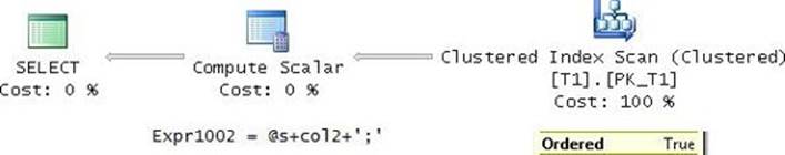
FIGURE 4-17 Plan for test 1 with assignment SELECT.
Observe that this plan scans the clustered index PK_T1, which is defined with col1 as the key, in order. Then the plan handles the assignments using the Compute Scalar operator. The execution of this plan resulted in the following output, which seems to be aligned with the expectation some have that the values will be concatenated based on the specified order:
String 1;String 2;String 3;String 4;String 5;String 6;String 7;String 8;String 9;String
10;String 11;String 12;String 13;String 14;String 15;String 16;String 17;String 18;String
19;String 20;String 21;String 22;String 23;String 24;String 25;String 26;String 27;String
28;String 29;String 30;String 31;String 32;String 33;String 34;String 35;String 36;String
37;String 38;String 39;String 40;String 41;String 42;String 43;String 44;String 45;String
46;String 47;String 48;String 49;String 50;String 51;String 52;String 53;String 54;String
55;String 56;String 57;String 58;String 59;String 60;String 61;String 62;String 63;String
64;String 65;String 66;String 67;String 68;String 69;String 70;String 71;String 72;String
73;String 74;String 75;String 76;String 77;String 78;String 79;String 80;String 81;String
82;String 83;String 84;String 85;String 86;String 87;String 88;String 89;String 90;String
91;String 92;String 93;String 94;String 95;String 96;String 97;String 98;String 99;String 100;
But as mentioned, there’s no documentation that provides you with such a guarantee. It just so happens that the optimizer’s choice resulted in such ordered strings.
Next, I added the following nonclustered index to the table and then ran the same assignment SELECT code:
CREATE NONCLUSTERED INDEX idx_nc_col2_i_col1 ON dbo.T1(col2, col1);
GO
DECLARE @s AS VARCHAR(MAX);
SET @s = '';
SELECT @s = @s + col2 + ';'
FROM dbo.T1
ORDER BY col1;
PRINT @s;
The plan I got for this execution of the query is shown in Figure 4-18.
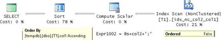
FIGURE 4-18 Plan for test 2 with assignment SELECT.
Observe that this time the optimizer chose to use the new index. It’s narrower than the clustered index because it contains only the interesting columns. But it doesn’t sort the rows like the query needs. So the plan performs an unordered scan of the index, and it adds a Sort operator as the last thing it does. The ironic thing is that the plan sorts the rows after the assignments already took place! Not only that, you don’t get the concatenated values in the order you need; rather, you get an intermediate state of the concatenation. When I ran this code, I got the following output:
String 100;
It’s sad to see how much production code exists out there that relies on this method, with the authors of it not realizing it’s not guaranteed to work the way they expect it to. And then something causes the optimizer to change how it optimizes the code, like a new index, a new service pack, and so on, and they get into trouble. You can save yourself a lot of grief if you stick to supported and well-defined techniques like the one based on the FOR XML PATH option.
Aggregate product
Computing an aggregate product is another classic type of custom aggregate calculation. It is commonly used in financial applications—for example, to compute compound interest rates.
With our Groups table, suppose you need to compute the product of the values in the val column per group. There’s an efficient solution for this task that is based on mathematics—specifically, logarithmic calculations. There are two sets of equations that are interesting for the solution:
logb(y) = x ⇔ y = bx
logb(xy) = logb(x) + logb(y) ⇔ xy = blogb(x) + logb(y)
The LOG function in T-SQL computes the logarithm of the first input using the second input as the base. If you don’t indicate the base, the function computes the natural logarithm of the first input (using e as the base, where e is an irrational constant approximately equal to 2.718281828).
The EXP function in T-SQL returns the exponent of the input value. That is, it returns e raised to the power of the input. So, EXP(10) is e10. This means that in the following pair of equations, one implies the other:
LOG(y) = x ⇔ EXP(x) = y
And therefore in the following pair of equations, one implies the other:
LOG(xy) = LOG(x) + LOG(y) ⇔ EXP(LOG(x) + LOG(y)) = xy
Expressed in T-SQL, here’s the query that computes the desired product:
SELECT groupid, ROUND(EXP(SUM(LOG(val))), 0) AS product
FROM dbo.Groups
GROUP BY groupid;
The rounding is required to correct errors caused by the imprecise nature of the floating-point calculations used by the LOG and EXP T-SQL functions. This query generates the following desired output:
groupid product
---------- ----------------------
a 42
b 693
c 960
If you want to also support zeros and negative values, things get trickier because the LOG function doesn’t support those. To see a demonstration of this, repopulate the Groups table by running the following code:
TRUNCATE TABLE dbo.Groups;
INSERT INTO dbo.Groups(groupid, memberid, string, val) VALUES
('a', 3, 'stra1', -6),
('a', 9, 'stra2', 7),
('b', 2, 'strb1', -3),
('b', 4, 'strb2', -7),
('b', 5, 'strb3', 3),
('b', 9, 'strb4', 11),
('c', 3, 'strc1', 8),
('c', 7, 'strc2', 0),
('c', 9, 'strc3', 12);
Try running the query against the new data:
SELECT groupid, ROUND(EXP(SUM(LOG(val))), 0) AS product
FROM dbo.Groups
GROUP BY groupid;
The query fails with the following error:
Msg 3623, Level 16, State 1, Line 1049
An invalid floating point operation occurred.
To deal with zeros and negatives correctly, you need a few things. Using the ISNULL function, you replace val with a NULL if it’s zero to avoid an error. You apply the original product calculation against the absolute values. Using the MIN aggregate and a CASE expression, you compute a flag (call it zero) that is 1 if you have at least one zero and 0 if you have none. Using the COUNT aggregate and a CASE expression, you compute a flag (call it negative) that is –1 if you have an odd number of negative values and 1 otherwise. Here’s the code applying these calculations:
SELECT groupid,
-- Replace 0 with NULL using NULLIF, apply product to absolute values
ROUND(EXP(SUM(LOG(ABS(NULLIF(val, 0))))), 0) AS product,
-- 0 if a 0 exists, 1 if not
MIN(CASE WHEN val = 0 THEN 0 ELSE 1 END) AS zero,
-- -1 if odd, 1 if even
CASE WHEN COUNT(CASE WHEN val < 0 THEN 1 END) % 2 > 0 THEN -1 ELSE 1 END AS negative
FROM dbo.Groups
GROUP BY groupid;
This code generates the following output:
groupid product zero negative
-------- -------- ----- ---------
a 42 1 -1
b 693 1 1
c 96 0 1
Then to get the correct product, you multiply the product of the absolute values by the zero flag and by the negative flag, like so:
SELECT groupid,
ROUND(EXP(SUM(LOG(ABS(NULLIF(val, 0))))), 0)
* MIN(CASE WHEN val = 0 THEN 0 ELSE 1 END)
* CASE WHEN COUNT(CASE WHEN val < 0 THEN 1 END) % 2 > 0 THEN -1 ELSE 1 END AS product
FROM dbo.Groups
GROUP BY groupid;
This query generates the following output:
groupid product
---------- ----------------------
a -42
b 693
c 0
If you like mathematical challenges, try computing the zero and negative flags mathematically without the use of CASE expressions. This can be done like so:
SELECT groupid,
ROUND(EXP(SUM(LOG(ABS(NULLIF(val, 0))))), 0) AS product,
MIN(SIGN(ABS(val))) AS zero,
SUM((1-SIGN(val))/2)%2*-2+1 AS negative
FROM dbo.Groups
GROUP BY groupid;
Putting it all together, you get the following query to compute the final product:
SELECT groupid,
ROUND(EXP(SUM(LOG(ABS(NULLIF(val, 0))))), 0)
* MIN(SIGN(ABS(val)))
* (SUM((1-SIGN(val))/2)%2*-2+1) AS product
FROM dbo.Groups
GROUP BY groupid;
Aggregate mode
Another example of a custom aggregate calculation is computing the mode of the distribution. Mode is the most frequently occurring value in a set. As an example, suppose you need to query the Sales.Orders table in the TSQLV3 database and find for each customer the employee who handled the most orders. That’s the employee ID that appears the most times in the customer’s orders. In case of ties in the count, you’re supposed to return the greater employee ID.
One approach to solving the task involves the following steps:
![]() Write a grouped query computing the count of orders per customer and employee.
Write a grouped query computing the count of orders per customer and employee.
![]() In the same grouped query, also compute a row number that is partitioned by the customer ID and ordered by the count descending and employee ID descending.
In the same grouped query, also compute a row number that is partitioned by the customer ID and ordered by the count descending and employee ID descending.
![]() Define a CTE based on the grouped query, and then in the outer query, filter only the rows with the row number 1.
Define a CTE based on the grouped query, and then in the outer query, filter only the rows with the row number 1.
Here’s the complete solution code:
USE TSQLV3;
WITH C AS
(
SELECT custid, empid, COUNT(*) AS cnt,
ROW_NUMBER() OVER(PARTITION BY custid
ORDER BY COUNT(*) DESC, empid DESC) AS rn
FROM Sales.Orders
GROUP BY custid, empid
)
SELECT custid, empid, cnt
FROM C
WHERE rn = 1;
This query generates the following output:
custid empid cnt
----------- ----------- -----------
1 4 2
2 3 2
3 3 3
4 4 4
5 3 6
...
If instead of breaking the ties you want to return all ties, you need to apply two changes to your solution. You need to use the RANK or DENSE_RANK functions (either one will work) and remove the employee ID from the window order clause. Here’s the revised code:
WITH C AS
(
SELECT custid, empid, COUNT(*) AS cnt,
RANK() OVER(PARTITION BY custid
ORDER BY COUNT(*) DESC) AS rn
FROM Sales.Orders
GROUP BY custid, empid
)
SELECT custid, empid, cnt
FROM C
WHERE rn = 1;
This code generates the following output:
custid empid cnt
----------- ----------- -----------
1 1 2
1 4 2
2 3 2
3 3 3
4 4 4
5 3 6
...
Observe that for customer 1 there are two employees who handled the maximum number of orders.
Going back to the original task that involves a tiebreaker, consider the optimization of the solution. Because the ROW_NUMBER function’s ordering is based in part on the result of the COUNT computation, there will be a sort operation of the entire input set in the query plan even if you create an index on (custid, empid). With a large amount of input, the sort will be expensive. There is a way to avoid the sort with an indexed view (as a challenge, see if you can figure out how), but what if you cannot afford one?
There’s an alternative solution that relies on a carry-along-sort concept based on grouping and string concatenation that can efficiently rely on an index on (custid, empid). The solution involves the following steps:
1. Write a grouped query that computes the count of orders per customer and employee.
2. In the same grouped query, compute a binary string made of the count converted to BINARY(4) concatenated with the employee ID, also converted to BINARY(4). Call the concatenated value binval.
3. Define a table expression based on the grouped query and name it D.
4. Write an outer query against D that groups the rows by customer ID. In that query, the result of the computation MAX(binval) contains the maximum count concatenated with the ID of the mode employee (with the maximum employee ID as the tiebreaker). Apply substring logic to extract the two parts and convert them back to the original types.
Here’s the complete solution code:
SELECT custid,
CAST(SUBSTRING(MAX(binval), 5, 4) AS INT) AS empid,
CAST(SUBSTRING(MAX(binval), 1, 4) AS INT) AS cnt
FROM (SELECT custid,
CAST(COUNT(*) AS BINARY(4)) + CAST(empid AS BINARY(4)) AS binval
FROM Sales.Orders
GROUP BY custid, empid) AS D
GROUP BY custid;
What’s nice about this solution is that both layers of grouping and aggregation can rely on the order of the aforementioned index. To compare the performance of the two solutions, I created a table called OrdersBig with 10,000,000 rows and an index called idx_custid_empid on (custid, empid). Figure 4-19 shows the plans that I got for both solutions against that table. The top plan is for the solution using the ROW_NUMBER function, and the bottom plan is for the solution based on the carry-along-sort concept.
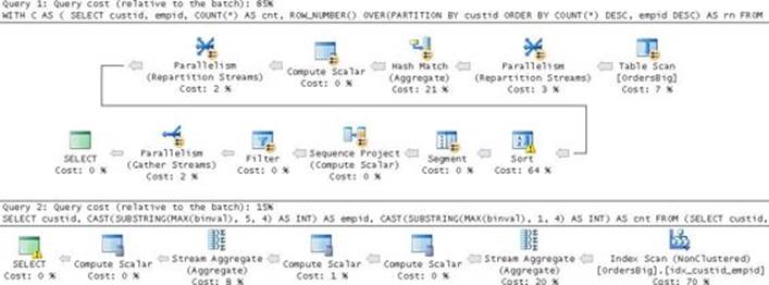
FIGURE 4-19 Plans for solutions to mode.
Notice the expensive Sort operator in the first plan before the calculation of the row numbers, and the absence of one in the second plan. The first solution took 15 seconds to complete in my test machine and the second completed in only 5 seconds.
Before concluding the section about custom aggregations, I want to mention that standard SQL defines a type of function called ordered set function, which at the date of this writing is not yet available in SQL Server. An ordered set function is a set function with ordering relevance that you can use in a grouped query. The standard defines a clause called WITHIN GROUP where you indicate the function’s ordering specification. There are multiple examples for functions that could be implemented as ordered set functions: aggregate string concatenation, percentiles, CLR aggregates, and so on. You can find a feature-enhancement request concerning ordered set functions here: https://connect.microsoft.com/SQLServer/feedback/details/728969.
Grouping sets
T-SQL supports a number of features that are related to the topic of grouping sets and that are useful for data-analysis purposes. Those features are the clauses GROUPING SETS, CUBE, and ROLLUP, as well as the functions GROUPING_ID and GROUPING.
To demonstrate these features, I’ll use a table called Orders in my examples. Run the following code to create the Orders table and populate it with sample data:
SET NOCOUNT ON;
USE tempdb;
IF OBJECT_ID(N'dbo.Orders', N'U') IS NOT NULL DROP TABLE dbo.Orders;
CREATE TABLE dbo.Orders
(
orderid INT NOT NULL,
orderdate DATETIME NOT NULL,
empid INT NOT NULL,
custid VARCHAR(5) NOT NULL,
qty INT NOT NULL,
CONSTRAINT PK_Orders PRIMARY KEY(orderid)
);
GO
INSERT INTO dbo.Orders
(orderid, orderdate, empid, custid, qty)
VALUES
(30001, '20120802', 3, 'A', 10),
(10001, '20121224', 1, 'A', 12),
(10005, '20121224', 1, 'B', 20),
(40001, '20130109', 4, 'A', 40),
(10006, '20130118', 1, 'C', 14),
(20001, '20130212', 2, 'B', 12),
(40005, '20140212', 4, 'A', 10),
(20002, '20140216', 2, 'C', 20),
(30003, '20140418', 3, 'B', 15),
(30004, '20120418', 3, 'C', 22),
(30007, '20120907', 3, 'D', 30);
Before describing features and functions, I’ll start by saying that the term grouping set simply describes the set of expressions you group by in a grouped query. For example, if you have a query that groups by custid, empid, YEAR(orderdate), your query defines the grouping set (custid, empid, YEAR(orderdate)). Nothing special so far.
Historically, T-SQL supported defining only one grouping set per query. With the features I’m about to describe, you can define multiple grouping sets in one query. The question is, why would you want to do that? There are a couple of reasons. One reason is that there are reports where you need to present more than one level of aggregation—for example, hierarchical time reports where you need to show daily, monthly, yearly, and grand totals. Another reason is to persist aggregates for different grouping sets in a table for fast retrieval. This is a classic need in data warehouses. There are other technologies that help you speed up analytical queries, like columnstore, but this technology requires the Enterprise edition of SQL Server.
The following sections describe the aforementioned features.
GROUPING SETS subclause
You use the GROUPING SETS clause to define multiple grouping sets in one query. You specify this clause as part of the GROUP BY clause. The GROUPING SETS clause has its own pair of parentheses, and each inner pair of parentheses represents a different grouping set. You separate grouping sets with commas. Without an inner pair of parentheses, each expression is considered a separate grouping set. An empty inner pair of parentheses defines only one group from the entire input set; in other words, you use them to compute grand aggregates.
As an example for using the GROUPING SETS clause, the following query defines four grouping sets:
SELECT custid, empid, YEAR(orderdate) AS orderyear, SUM(qty) AS qty
FROM dbo.Orders
GROUP BY GROUPING SETS
(
( custid, empid, YEAR(orderdate) ),
( custid, YEAR(orderdate) ),
( empid, YEAR(orderdate) ),
()
);
But then there’s the question of how the result sets for the different grouping sets can be combined if they have different structures. The solution is to use NULLs as placeholders in columns that are not part of the grouping set that the result row is associated with. Here’s the output of the preceding query:
custid empid orderyear qty
------ ----------- ----------- -----------
A 1 2012 12
B 1 2012 20
NULL 1 2012 32
C 1 2013 14
NULL 1 2013 14
B 2 2013 12
NULL 2 2013 12
C 2 2014 20
NULL 2 2014 20
A 3 2012 10
C 3 2012 22
D 3 2012 30
NULL 3 2012 62
B 3 2014 15
NULL 3 2014 15
A 4 2013 40
NULL 4 2013 40
A 4 2014 10
NULL 4 2014 10
NULL NULL NULL 205
A NULL 2012 22
B NULL 2012 20
C NULL 2012 22
D NULL 2012 30
A NULL 2013 40
B NULL 2013 12
C NULL 2013 14
A NULL 2014 10
B NULL 2014 15
C NULL 2014 20
The rows that have values in custid, empid, and orderyear are related to the grouping set ( custid, empid, YEAR(orderdate) ). Similarly, the rows that have values in empid and orderyear and NULLs in custid are related to the grouping set ( empid, YEAR(orderdate) ), and so on.
If you want to get the same result without the GROUPING SETS clause, you need to write four grouped queries and unify their results, like so:
SELECT custid, empid, YEAR(orderdate) AS orderyear, SUM(qty) AS qty
FROM dbo.Orders
GROUP BY custid, empid, YEAR(orderdate)
UNION ALL
SELECT custid, NULL AS empid, YEAR(orderdate) AS orderyear, SUM(qty) AS qty
FROM dbo.Orders
GROUP BY custid, YEAR(orderdate)
UNION ALL
SELECT NULL AS custid, empid, YEAR(orderdate) AS orderyear, SUM(qty) AS qty
FROM dbo.Orders
GROUP BY empid, YEAR(orderdate)
UNION ALL
SELECT NULL AS custid, NULL AS empid, NULL AS orderyear, SUM(qty) AS qty
FROM dbo.Orders;
The GROUPING SETS clause gives you a couple of advantages over multiple queries. Obviously, the code is much shorter. In addition, it gets optimized better. With four queries, the data will be scanned four times. With the GROUPING SETS clause, the optimizer analyzes the grouping sets and tries to minimize the number of scans by rolling up aggregates. To see this optimization technique in action, examine the query plan shown in Figure 4-20 for the query with the GROUPING SETS clause.
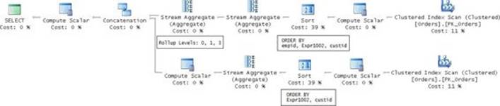
FIGURE 4-20 Plan for a query with GROUPING SETS.
Observe that the data is scanned only twice. The top branch of the plan, from right to left, starts by scanning the clustered index. It then computes a scalar called Expr1002 representing the result of the computation YEAR(orderdate). Because I did not prepare any indexes to support the grouping and aggregation, the optimizer adds a Sort operator that orders the rows by empid, YEAR(orderdate), custid. You can avoid this sort by creating a supporting index, as I’ll demonstrate shortly. Based on this order, in a rollup fashion, all grouping sets representing leading combinations can be computed. The rolled-up levels are numbered using a zero-based offset from lower to higher:
![]() Level 0: empid, YEAR(orderdate), custid
Level 0: empid, YEAR(orderdate), custid
![]() Level 1: empid, YEAR(orderdate)
Level 1: empid, YEAR(orderdate)
![]() Level 2: empid
Level 2: empid
![]() Level 3: ()
Level 3: ()
The first aggregate operator to the left of the Sort operator represents the base grouping set (level 0). The second aggregate operator is responsible for the rolling up of the aggregates. If you examine the query, you will notice that the GROUPING SETS clause defines three of the aforementioned grouping sets: the ones with levels 0, 1, and 3, but not 2. So when looking at the properties of the second aggregate operator, the property Rollup Levels will report only the needed levels.
The query defines an additional grouping set ( custid, YEAR(orderdate) ) that cannot be computed based on the order in the first branch of the plan. So a second branch in the plan (the bottom one) scans the data again, sorts it by YEAR(orderdate), custid, and then computes the aggregates for the remaining grouping set. There’s no need for a second aggregate operator because only one grouping set remains; so there’s no rolling up to do.
As mentioned, you can avoid explicit sorting in the plan by preparing supporting indexes. In our case, one of the elements is a result of a computation, so you can add a computed column based on that computation and then make it part of your indexes. You want the indexes to be covering, so don’t forget to include the aggregated column (qty in our case). Here’s the code to add the computed column and the supporting indexes:
ALTER TABLE dbo.Orders ADD orderyear AS YEAR(orderdate);
GO
CREATE INDEX idx_eid_oy_cid_i_qty ON dbo.Orders(empid, orderyear, custid) INCLUDE(qty);
CREATE INDEX idx_oy_cid_i_qty ON dbo.Orders(orderyear, custid) INCLUDE(qty);
Run the query again, and you will get the plan shown in Figure 4-21.
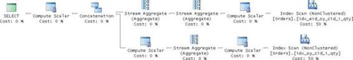
FIGURE 4-21 Plan for a query with GROUPING SETS after adding index.
The supporting indexes are scanned in order, and therefore no sort operation is required this time.
CUBE and ROLLUP clauses
The CUBE and ROLLUP clauses are simply shortcuts for the GROUPING SETS clause. When you need to define a large number of grouping sets (you’re allowed to define up to 4,096), it’s nice if you can avoid actually listing all of them.
Starting with the CUBE clause, suppose you have a set of expressions and you want to define all possible grouping sets from them. In mathematics, this is what’s known as the power set of a set. It’s the set of all subsets that are formed from the original set’s elements. For a set with cardinality N, the power set has cardinality 2N. For example, for a set with 10 elements you get a power set of 1,024 subsets, including the original set and the empty set. That’s pretty much what CUBE is about. You provide it with a set of expressions as inputs, and you get the equivalent of a GROUPING SETS clause with all grouping sets that can be formed from the input expressions. As a simple example, here’s a query with a CUBE clause with two input expressions:
SELECT custid, empid, SUM(qty) AS qty
FROM dbo.Orders
GROUP BY CUBE(custid, empid);
This query is equivalent to the following query, which uses a GROUPING SETS clause with all possible grouping sets:
SELECT custid, empid, SUM(qty) AS qty
FROM dbo.Orders
GROUP BY GROUPING SETS
(
( custid, empid ),
( custid ),
( empid ),
()
);
With two input elements to the CUBE clause, the power set contains four grouping sets.
As for the ROLLUP clause, it’s also a shortcut, but one that assumes that the inputs form a hierarchy like time, location, and so on. You get only grouping sets that are formed by leading combinations of expressions. Consider the following query as an example:
SELECT
YEAR(orderdate) AS orderyear,
MONTH(orderdate) AS ordermonth,
DAY(orderdate) AS orderday,
SUM(qty) AS qty
FROM dbo.Orders
GROUP BY
ROLLUP(YEAR(orderdate), MONTH(orderdate), DAY(orderdate));
For N elements, there are N + 1 leading combinations (including the empty set). The preceding query has a ROLLUP clause with three inputs, and therefore it is equivalent to the following query with a GROUPING SETS clause defining four grouping sets:
SELECT
YEAR(orderdate) AS orderyear,
MONTH(orderdate) AS ordermonth,
DAY(orderdate) AS orderday,
SUM(qty) AS qty
FROM dbo.Orders
GROUP BY
GROUPING SETS
(
( YEAR(orderdate), MONTH(orderdate), DAY(orderdate) ),
( YEAR(orderdate), MONTH(orderdate) ),
( YEAR(orderdate) ),
()
);
What’s interesting about the ROLLUP clause is how nicely the optimization of the feature is aligned with its logical design. Recall the rollup concept in the optimization of grouping sets? One ROLLUP clause can be optimized with a single scan based on one order (requiring either an actual sort or an ordered scan of a supporting index). Figure 4-22 has the plan for the preceding ROLLUP query.
![]()
FIGURE 4-22 Plan for a query with ROLLUP.
![]() Tip
Tip
A little known fact about the CUBE and ROLLUP clauses is that their inputs are not limited to only scalar elements; rather, they can be sets. For example, CUBE( (a, b), (x, y) ) assumes two input sets: (a, b) and (x, y), generating four grouping sets: (a, b, c, d), (a, b), (x, y), ().
Grouping sets algebra
One of the interesting aspects in the design of queries with grouping sets is that you can apply algebra-like operations between the clauses that define them (GROUPING SETS, CUBE, and ROLLUP). You have both multiplication and addition operations.
You achieve multiplication simply by putting a comma between the clauses. For example, consider the following query:
SELECT
custid,
empid,
YEAR(orderdate) AS orderyear,
MONTH(orderdate) AS ordermonth,
SUM(qty) AS qty
FROM dbo.Orders
GROUP BY
GROUPING SETS
(
( custid, empid ),
( custid ),
( empid )
),
ROLLUP(YEAR(orderdate), MONTH(orderdate), DAY(orderdate));
The GROUPING SETS clause defines three grouping sets, and the ROLLUP clause defines four. The multiplication operation results in 12 grouping sets. A typical use case is multiplying a number of ROLLUP clauses, each representing a different dimension hierarchy (time, location, and so on).
To apply addition, you place a ROLLUP or CUBE clause as an additional element within a GROUPING SETS clause, like so:
SELECT
custid,
empid,
YEAR(orderdate) AS orderyear,
MONTH(orderdate) AS ordermonth,
SUM(qty) AS qty
FROM dbo.Orders
GROUP BY
GROUPING SETS
(
( custid, empid ),
( custid ),
( empid ),
ROLLUP(YEAR(orderdate), MONTH(orderdate), DAY(orderdate))
);
Here you add the four grouping sets that are defined by the ROLLUP clause to the three explicit ones that are defined within the GROUPING SETS clause, getting seven grouping sets in total. So remember, when the comma appears between clauses it behaves like multiplication; when it appears within a GROUPING SETS clause, it behaves like addition.
Materializing grouping sets
As mentioned at the beginning of the section, one of the use cases of the features that allow you to define multiple grouping sets in one query is to persist aggregates that are expensive to compute to speed up retrievals. This is usually done nightly, allowing fast retrievals during the day.
Once persisted, users will typically ask for aggregates that are related to one grouping set at a time. The question is, how do you filter only the rows that are associated with one grouping set? You need a mechanism that identifies a grouping set uniquely. One option is to form a filter with IS NULL and IS NOT NULL predicates against all grouping columns. But there are two problems with this approach. One, it’s awkward. Two, if a grouping column allows NULLs in the table, the result will include false positives.
There’s an elegant solution in the form of a function called GROUPING_ID. You provide the function with all grouping columns as inputs. The function returns an integer bitmap where each bit represents the respective input, with the rightmost bit representing the rightmost input. The bit is set if the respective column is not part of the grouping set (namely, it’s an aggregate) and is not set when it is.
As an example, consider the following query:
SELECT
GROUPING_ID( custid, empid, YEAR(orderdate), MONTH(orderdate), DAY(orderdate) ) AS grp_id,
custid, empid,
YEAR(orderdate) AS orderyear,
MONTH(orderdate) AS ordermonth,
DAY(orderdate) AS orderday,
SUM(qty) AS qty
FROM dbo.Orders
GROUP BY
CUBE(custid, empid),
ROLLUP(YEAR(orderdate), MONTH(orderdate), DAY(orderdate));
This query generates the following output, with an extra header with the respective bit values added manually on top for clarity:
bit value 16 8 4 2 1
---------- ------ ------ ---------- ----------- --------- ----
grp_id custid empid orderyear ordermonth orderday qty
---------- ------ ------ ---------- ----------- --------- -----
...
25 NULL NULL 2014 4 NULL 15
27 NULL NULL 2014 NULL NULL 45
31 NULL NULL NULL NULL NULL 205
8 A NULL 2012 8 2 10
...
Take, for example, the row where the function returned the value 25. This row is associated with the grouping set ( YEAR(orderdate), MONTH(orderdate) ). The respective bits are the ones with the values 4 and 2, and those are the bits that are not set. The bits for the remaining elements—custid, empid and DAY(orderdate)—are set. Those are the bits with the bit values 16, 8, and 1, respectively. Sum the values of those bits and you get 25.
You’re the one who determines which bit represents which grouping element by providing the elements as inputs to the function in a specific order. Therefore, when the user will request a certain grouping set, you will be able to calculate the integer bitmap value that uniquely identifies that grouping set.
In the query you use to persist the aggregates, you include the computation of the integer bitmap (call the result column grp_id) to uniquely identify the grouping set that each result row is associated with. Also, you create a clustered index on the table with the grp_id column as the leading key to support efficient retrieval of aggregates that are related to a single requested grouping set.
Here’s code to persist the aggregates for the last query in a table called MyGroupingSets and to create the aforementioned supporting index:
USE tempdb;
IF OBJECT_ID(N'dbo.MyGroupingSets', N'U') IS NOT NULL DROP TABLE dbo.MyGroupingSets;
GO
SELECT
GROUPING_ID(
custid, empid,
YEAR(orderdate), MONTH(orderdate), DAY(orderdate) ) AS grp_id,
custid, empid,
YEAR(orderdate) AS orderyear,
MONTH(orderdate) AS ordermonth,
DAY(orderdate) AS orderday,
SUM(qty) AS qty
INTO dbo.MyGroupingSets
FROM dbo.Orders
GROUP BY
CUBE(custid, empid),
ROLLUP(YEAR(orderdate), MONTH(orderdate), DAY(orderdate));
CREATE UNIQUE CLUSTERED INDEX idx_cl_groupingsets
ON dbo.MyGroupingSets(grp_id, custid, empid, orderyear, ordermonth, orderday);
Suppose that a user requests the aggregates that are associated with the grouping set ( custid, YEAR(orderdate), MONTH(orderdate) ). The bit values of the other grouping elements (empid and DAY(orderdate)) are 8 and 1, respectively. So you query the table filtering grp_id 9, like so:
SELECT *
FROM dbo.MyGroupingSets
WHERE grp_id = 9;
Because the clustered index on the table has the grp_id column as the leading key, you get an efficient plan that performs a seek within that index, as shown in Figure 4-23.
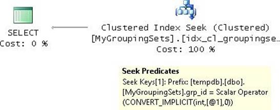
FIGURE 4-23 Plan for a query returning a single grouping.
If your source is very large and the full processing of the aggregates takes a long time, you will probably want to avoid doing the full processing every night. You will want to run the full processing once, and then every night run an incremental update process. That’s, of course, assuming that the aggregated measures are additive.
As an example, suppose that today was April 19, 2014. The persisted aggregates hold data until the 18th, inclusive. Here’s code representing new orders added on the 19th:
INSERT INTO dbo.Orders
(orderid, orderdate, empid, custid, qty)
VALUES
(50001, '20140419', 1, 'A', 10),
(50002, '20140419', 1, 'B', 30),
(50003, '20140419', 2, 'A', 20),
(50004, '20140419', 2, 'B', 5),
(50005, '20140419', 3, 'A', 15);
In the nightly process, you want to merge the aggregates for the last day with the existing ones. You want to update the target row by incrementing the value if the key already exists. You want to insert a new row if the key doesn’t exist. To achieve this, you define a CTE called LastDay that computes the aggregates for the last day. You provide the LastDay CTE as the source to the MERGE statement. The MERGE statement will use the EXISTS predicate with an INTERSECT set operator to check if the source key list is matched by a target key list. This will not require you to add special logic for correct NULL treatment. When the EXISTS predicate returns true, the MERGE statement will update the target row by incrementing the value. When the predicate returns false, the MERGE statement will insert a new row. Here’s the implementation of such a MERGE statement:
WITH LastDay AS
(
SELECT
GROUPING_ID(
custid, empid,
YEAR(orderdate), MONTH(orderdate), DAY(orderdate) ) AS grp_id,
custid, empid,
YEAR(orderdate) AS orderyear,
MONTH(orderdate) AS ordermonth,
DAY(orderdate) AS orderday,
SUM(qty) AS qty
FROM dbo.Orders
WHERE orderdate = '20140419'
GROUP BY
CUBE(custid, empid),
ROLLUP(YEAR(orderdate), MONTH(orderdate), DAY(orderdate))
)
MERGE INTO dbo.MyGroupingSets AS TGT
USING LastDay AS SRC
ON EXISTS(
SELECT SRC.grp_id, SRC.orderyear, SRC.ordermonth, SRC.orderday, SRC.custid, SRC.empid
INTERSECT
SELECT TGT.grp_id, TGT.orderyear, TGT.ordermonth, TGT.orderday, TGT.custid, TGT.empid)
WHEN MATCHED THEN
UPDATE SET
TGT.qty += SRC.qty
WHEN NOT MATCHED THEN
INSERT (grp_id, custid, empid, orderyear, ordermonth, orderday)
VALUES (SRC.grp_id, SRC.custid, SRC.empid, SRC.orderyear, SRC.ordermonth, SRC.orderday);
Chapter 6, “Data modification,” has more information about the MERGE statement.
Sorting
Remember that if you don’t specify a presentation ORDER BY clause in a query, you don’t have any assurances regarding presentation order. Without an ORDER BY clause, even if the rows seem to come back in a certain order, it doesn’t mean that you have any guarantees.
For example, suppose you have a query with a ROLLUP clause computing daily, monthly, yearly, and grand aggregates. The optimizer normally optimizes the ROLLUP clause with two Stream Aggregate operators based on the order of the elements in the clause. So there’s likelihood that even without an ORDER BY clause you will get the rows presented based on the order of the time hierarchy. But that’s not something you want to rely on as guaranteed behavior. Optimization can change. The only way to truly guarantee output order is with an explicit ORDER BY clause.
If you didn’t have multiple levels of aggregation, but rather only daily ones, you would simply order the rows by the time vector YEAR(orderdate), MONTH(orderdate), DAY(orderdate). But because you have daily, monthly, yearly, and grand totals, ordering based on the time hierarchy is trickier. A tool that can help you with this is a function called GROUPING. It’s similar to the GROUPING_ID function, but it supports only one input. Like GROUPING_ID, the GROUPING function returns a 0 when the element is a detail element (part of the grouping set) and 1 when it’s an aggregate (not part of the grouping set). So, to place the rows with a detail year before the row with the grand total, you place GROUPING(YEAR(orderdate)) before YEAR(orderdate) in the ORDER BY clause. The same goes for the month and day elements.
The following query demonstrates how to apply this logic to get the detail sorted before the aggregate in each level (days in the month, then month total; months in the year, then yearly total; years, then grand total):
SELECT
YEAR(orderdate) AS orderyear,
MONTH(orderdate) AS ordermonth,
DAY(orderdate) AS orderday,
SUM(qty) AS totalqty
FROM dbo.Orders
GROUP BY
ROLLUP(YEAR(orderdate), MONTH(orderdate), DAY(orderdate))
ORDER BY
GROUPING(YEAR(orderdate)) , YEAR(orderdate),
GROUPING(MONTH(orderdate)), MONTH(orderdate),
GROUPING(DAY(orderdate)) , DAY(orderdate);
This query generates the following output:
orderyear ordermonth orderday totalqty
----------- ----------- ----------- -----------
2012 4 18 22
2012 4 NULL 22
2012 8 2 10
2012 8 NULL 10
2012 9 7 30
2012 9 NULL 30
2012 12 24 32
2012 12 NULL 32
2012 NULL NULL 94
2013 1 9 40
2013 1 18 14
2013 1 NULL 54
2013 2 12 12
2013 2 NULL 12
2013 NULL NULL 66
2014 2 12 10
2014 2 16 20
2014 2 NULL 30
2014 4 18 15
2014 4 19 80
2014 4 NULL 95
2014 NULL NULL 125
NULL NULL NULL 285
Now the presentation order is guaranteed, and it does not just happen to be this order because of optimization reasons.
Conclusion
This chapter covered quite a lot of ground concerning data analysis. It started with coverage of the profound window functions, describing the different types, as well as practical uses like handling gaps and islands problems. The chapter continued by covering techniques to handle pivoting and unpivoting tasks, showing both solutions that rely on standard methods and ones based on the proprietary PIVOT and UNPIVOT operators. The chapter then covered different ways to handle custom aggregate calculations like string concatenation and product. Finally, the chapter covered a number of features you can use to compute aggregates for multiple grouping sets in the same query.