T-SQL Querying (2015)
Chapter 5. TOP and OFFSET-FETCH
Classic filters in SQL like ON, WHERE, and HAVING are based on predicates. TOP and OFFSET-FETCH are filters that are based on a different concept: you indicate order and how many rows to filter based on that order. Many filtering tasks are defined based on order and a required number of rows. It’s certainly good to have language support in T-SQL that allows you to phrase the request in a manner that is similar to the way you think about the task.
This chapter starts with the logical design aspects of the filters. It then uses a paging scenario to demonstrate their optimization. The chapter also covers the use of TOP with modification statements. Finally, the chapter demonstrates the use of TOP and OFFSET-FETCH in solving practical problems like top N per group and median.
The TOP and OFFSET-FETCH filters
You use the TOP and OFFSET-FETCH filters to implement filtering requirements in your queries in an intuitive manner. The TOP filter is a proprietary feature in T-SQL, whereas the OFFSET-FETCH filter is a standard feature. T-SQL started supporting OFFSET-FETCH with Microsoft SQL Server 2012. As of SQL Server 2014, the implementation of OFFSET-FETCH in T-SQL is still missing a couple of standard elements—interestingly, ones that are available with TOP. With the current implementation, each of the filters has capabilities that are not supported by the other.
I’ll start by describing the logical design aspects of TOP and then cover those of OFFSET-FETCH.
The TOP filter
The TOP filter is a commonly used construct in T-SQL. Its popularity probably can be attributed to the fact that its design is so well aligned with the way many filtering requirements are expressed—for example, “Return the three most recent orders.” In this request, the order for the filter is based on orderdate, descending, and the number of rows you want to filter based on this order is 3.
You specify the TOP option in the SELECT list with an input value typed as BIGINT indicating how many rows you want to filter. You provide the ordering specification in the classic ORDER BY clause. For example, you use the following query to get the three most recent orders.
USE TSQLV3;
SELECT TOP (3) orderid, orderdate, custid, empid
FROM Sales.Orders
ORDER BY orderdate DESC;
I got the following output from this query:
orderid orderdate custid empid
----------- ---------- ----------- -----------
11077 2015-05-06 65 1
11076 2015-05-06 9 4
11075 2015-05-06 68 8
Instead of specifying the number of rows you want to filter, you can use TOP to specify the percent (of the total number of rows in the query result). You do so by providing a value in the range 0 through 100 (typed as FLOAT) and add the PERCENT keyword. For example, in the following query you request to filter one percent of the rows:
SELECT TOP (1) PERCENT orderid, orderdate, custid, empid
FROM Sales.Orders
ORDER BY orderdate DESC;
SQL Server rounds up the number of rows computed based on the input percent. For example, the result of 1 percent applied to 830 rows in the Orders table is 8.3. Rounding up this number, you get 9. Here’s the output I got for this query:
orderid orderdate custid empid
----------- ---------- ----------- -----------
11074 2015-05-06 73 7
11075 2015-05-06 68 8
11076 2015-05-06 9 4
11077 2015-05-06 65 1
11070 2015-05-05 44 2
11071 2015-05-05 46 1
11072 2015-05-05 20 4
11073 2015-05-05 58 2
11067 2015-05-04 17 1
Note that to translate the input percent to a number of rows, SQL Server has to first figure out the count of rows in the query result, and this usually requires extra work.
Interestingly, ordering specification is optional for the TOP filter. For example, consider the following query:
SELECT TOP (3) orderid, orderdate, custid, empid
FROM Sales.Orders;
I got the following output from this query:
orderid orderdate custid empid
----------- ---------- ----------- -----------
10248 2013-07-04 85 5
10249 2013-07-05 79 6
10250 2013-07-08 34 4
The selection of which three rows to return is nondeterministic. This means that if you run the query again, without the underlying data changing, theoretically you could get a different set of three rows. In practice, the row selection will depend on physical conditions like optimization choices, storage engine choices, data layout, and other factors. If you actually run the query multiple times, as long as those physical conditions don’t change, there’s some likelihood you will keep getting the same results. But it is critical to understand the “physical data independence” principle from the relational model, and remember that at the logical level you do not have a guarantee for repeatable results. Without ordering specification, you should consider the order as being arbitrary, resulting in a nondeterministic row selection.
Even when you do provide ordering specification, it doesn’t mean that the query is deterministic. For example, an earlier TOP query used orderdate, DESC as the ordering specification. The orderdate column is not unique; therefore, the selection between rows with the same order date is nondeterministic. So what do you do in cases where you must guarantee determinism? There are two options: using WITH TIES or unique ordering.
The WITH TIES option causes ties to be included in the result. Here’s how you apply it to our example:
SELECT TOP (3) WITH TIES orderid, orderdate, custid, empid
FROM Sales.Orders
ORDER BY orderdate DESC;
Here’s the result I got from this query:
orderid orderdate custid empid
----------- ---------- ----------- -----------
11077 2015-05-06 65 1
11076 2015-05-06 9 4
11075 2015-05-06 68 8
11074 2015-05-06 73 7
SQL Server filters the three rows with the most recent order dates, plus it includes all other rows that have the same order date as in the last row. As a result, you can get more rows than the number you specified. In this query, you specified you wanted to filter three rows but ended up getting four. What’s interesting to note here is that the row selection is now deterministic, but the presentation order between rows with the same order date is nondeterministic.
A quick puzzle
What is the following query looking for? (Try to figure this out yourself before looking at the answer.)
SELECT TOP (1) WITH TIES orderid, orderdate, custid, empid
FROM Sales.Orders
ORDER BY ROW_NUMBER() OVER(PARTITION BY custid ORDER BY orderdate DESC, orderid DESC);
Answer: This query returns the most recent order for each customer.
The second method to guarantee a deterministic result is to make the ordering specification unique by adding a tiebreaker. For example, you could add orderid, DESC as the tiebreaker in our example. This means that, in the case of ties in the order date values, a row with a higher order ID value is preferred to a row with a lower one. Here’s our query with the tiebreaker applied:
SELECT TOP (3) orderid, orderdate, custid, empid
FROM Sales.Orders
ORDER BY orderdate DESC, orderid DESC;
This query generates the following output:
orderid orderdate custid empid
----------- ---------- ----------- -----------
11077 2015-05-06 65 1
11076 2015-05-06 9 4
11075 2015-05-06 68 8
Use of unique ordering makes both the row selection and presentation ordering deterministic. The result set as well as the presentation ordering of the rows are guaranteed to be repeatable so long as the underlying data doesn’t change.
If you have a case where you need to filter a certain number of rows but truly don’t care about order, it could be a good idea to specify ORDER BY (SELECT NULL), like so:
SELECT TOP (3) orderid, orderdate, custid, empid
FROM Sales.Orders
ORDER BY (SELECT NULL);
This way, you let everyone know your choice of arbitrary order is intentional, which helps to avoid confusion and doubt.
As a reminder of what I explained in Chapter 1, “Logical query processing,” about the TOP and OFFSET-FETCH filters, presentation order is guaranteed only if the outer query has an ORDER BY clause. For example, in the following query presentation, ordering is not guaranteed:
SELECT orderid, orderdate, custid, empid
FROM ( SELECT TOP (3) orderid, orderdate, custid, empid
FROM Sales.Orders
ORDER BY orderdate DESC, orderid DESC ) AS D;
To provide a presentation-ordering guarantee, you must specify an ORDER BY clause in the outer query, like so:
SELECT orderid, orderdate, custid, empid
FROM ( SELECT TOP (3) orderid, orderdate, custid, empid
FROM Sales.Orders
ORDER BY orderdate DESC, orderid DESC ) AS D
ORDER BY orderdate DESC, orderid DESC;
The OFFSET-FETCH filter
The OFFSET-FETCH filter is a standard feature designed similar to TOP but with an extra element. You can specify how many rows you want to skip before specifying how many rows you want to filter.
As you could have guessed, this feature can be handy in implementing paging solutions—that is, returning a result to the user one chunk at a time upon request when the full result set is too long to fit in one screen or web page.
The OFFSET-FETCH filter requires an ORDER BY clause to exist, and it is specified right after it. You start by indicating how many rows to skip in an OFFSET clause, followed by how many rows to filter in a FETCH clause. For example, based on the indicated order, the following query skips the first 50 rows and filters the next 25 rows:
SELECT orderid, orderdate, custid, empid
FROM Sales.Orders
ORDER BY orderdate DESC, orderid DESC
OFFSET 50 ROWS FETCH NEXT 25 ROWS ONLY;
In other words, the query filters rows 51 through 75. In paging terms, assuming a page size of 25 rows, this query returns the third page.
To allow natural declarative language, you can use the keyword FIRST instead of NEXT if you like, though the meaning is the same. Using FIRST could be more intuitive if you’re not skipping any rows. Even if you don’t want to skip any rows, T-SQL still makes it mandatory to specify the OFFSET clause (with 0 ROWS) to avoid parsing ambiguity. Similarly, instead of using the plural form of the keyword ROWS, you can use the singular form ROW in both the OFFSET and the FETCH clauses. This is more natural if you need to skip or filter only one row.
If you’re curious what the purpose of the keyword ONLY is, it means not to include ties. Standard SQL defines the alternative WITH TIES; however, T-SQL doesn’t support it yet. Similarly, standard SQL defines the PERCENT option, but T-SQL doesn’t support it yet either. These two missing options are available with the TOP filter.
As mentioned, the OFFSET-FETCH filter requires an ORDER BY clause. If you want to use arbitrary order, like TOP without an ORDER BY clause, you can use the trick with ORDER BY (SELECT NULL), like so:
SELECT orderid, orderdate, custid, empid
FROM Sales.Orders
ORDER BY (SELECT NULL)
OFFSET 0 ROWS FETCH NEXT 3 ROWS ONLY;
The FETCH clause is optional. If you want to skip a certain number of rows but not limit how many rows to return, simply don’t indicate a FETCH clause. For example, the following query skips 50 rows but doesn’t limit the number of returned rows:
SELECT orderid, orderdate, custid, empid
FROM Sales.Orders
ORDER BY orderdate DESC, orderid DESC
OFFSET 50 ROWS;
Concerning presentation ordering, the behavior is the same as with the TOP filter; namely, with OFFSET-FETCH also, presentation ordering is guaranteed only if the outermost query has an ORDER BY clause.
Optimization of filters demonstrated through paging
So far, I described the logical design aspects of the TOP and OFFSET-FETCH filters. In this section, I’m going to cover optimization aspects. I’ll do so by looking at different paging solutions. I’ll describe two paging solutions using the TOP filter, a solution using the OFFSET-FETCH filter, and a solution using the ROW_NUMBER function.
In all cases, regardless of which filtering option you use for your paging solution, an index on the ordering elements is crucial for good performance. Often you will get good performance even when the index is not a covering one. Curiously, sometimes you will get better performance when the index isn’t covering. I’ll provide the details in the specific implementations.
I’ll use the Orders table from the PerformanceV3 database in my examples. Suppose you need to implement a paging solution returning one page of orders at a time, based on orderid as the sort key. The table has a nonclustered index called PK_Orders defined with orderid as the key. This index is not a covering one with respect to the paging queries I will demonstrate.
Optimization of TOP
There are a couple of strategies you can use to implement paging solutions with TOP. One is an anchor-based strategy, and the other is TOP over TOP (nested TOP queries).
The anchor-based strategy allows the user to visit adjacent pages progressively. You define a stored procedure that when given the sort key of the last row from the previous page, returns the next page. Here’s an implementation of such a procedure:
USE PerformanceV3;
IF OBJECT_ID(N'dbo.GetPage', N'P') IS NOT NULL DROP PROC dbo.GetPage;
GO
CREATE PROC dbo.GetPage
@orderid AS INT = 0, -- anchor sort key
@pagesize AS BIGINT = 25
AS
SELECT TOP (@pagesize) orderid, orderdate, custid, empid
FROM dbo.Orders
WHERE orderid > @orderid
ORDER BY orderid;
GO
Here I’m assuming that only positive order IDs are supported. Of course, you can implement such an integrity rule with a CHECK constraint. The query uses the WHERE clause to filter only orders with order IDs that are greater than the input anchor sort key. From the remaining rows, using TOP, the query filters the first @pagesize rows based on orderid ordering.
Use the following code to request the first page of orders:
EXEC dbo.GetPage @pagesize = 25;
I got the following result (but yours may vary because of the randomization aspects used in the creation of the sample data):
orderid orderdate custid empid
----------- ---------- ----------- -----------
1 2011-01-01 C0000005758 205
2 2011-01-01 C0000015925 251
...
24 2011-01-01 C0000003541 316
25 2011-01-01 C0000005636 256
In this example, the last sort key in the first page is 25. Therefore, to request the second page of orders, you pass 25 as the input anchor sort key, like so:
EXEC dbo.GetPage @orderid = 25, @pagesize = 25;
Of course, in practice the last sort key in the first page could be different than 25, but in my sample data the keys start with 1 and are sequential. I got the following result when running this code:
orderid orderdate custid empid
----------- ---------- ----------- -----------
26 2011-01-01 C0000017397 332
27 2011-01-01 C0000012629 27
28 2011-01-01 C0000016429 53
...
49 2011-01-01 C0000015415 95
50 2010-12-06 C0000008667 117
To ask for the third page of orders, you pass 50 as the input sort key in the next page request:
EXEC dbo.GetPage @orderid = 50, @pagesize = 25;
I got the following output for the execution of this code:
orderid orderdate custid empid
----------- ---------- ----------- -----------
51 2011-01-01 C0000000797 438
52 2011-01-01 C0000015945 47
53 2011-01-01 C0000013558 364
...
74 2011-01-01 C0000019720 249
75 2011-01-01 C0000000807 160
The execution plan for the query is shown in Figure 5-1. I’ll assume the inputs represent the last procedure call with the request for the third page.
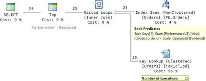
FIGURE 5-1 Plan for TOP with a single anchor sort key.
I’ll describe the execution of this plan based on data flow order (right to left). But keep in mind that the API call order is actually left to right, starting with the root node (SELECT). I’ll explain why that’s important to remember shortly.
The Index Seek operator performs a seek in the index PK_Orders to the first leaf row that satisfies the Start property of the Seek Predicates property: orderid > @orderid. In the third execution of the procedure, @orderid is 50. Then the Index Seek operator continues with a range scan in the index leaf based on the seek predicate. Absent a Prefix property of the Seek Predicates property, the range scan normally continues until the tail of the index leaf. However, as mentioned, the internal API call order is done from left to right. The Top operator has a property called Top Expression, which is set in the plan to @pagesize (25, in our case). This property tells the Top operator how many rows to request from the Nested Loops operator to its right. In turn, the Nested Loops operator requests the specified number of rows (25, in our case) from the Index Seek operator to its right. For each row returned from the Index Seek Operator, Nested Loops executes the Key Lookup operator to collect the remaining elements from the respective data row. This means that the range scan doesn’t proceed beyond the 25th row, and this also means that the Key Lookup operator is executed 25 times.
Not only is the range scan in the Index Seek operator cut short because of TOP’s row goal (Top Expression property), the query optimizer needs to adjust the costs of the affected operators based on that row goal. This aspect of optimization is described in detail in an excellent article by Paul White: “Inside the Optimizer: Row Goals In Depth.” The article can be found here: http://sqlblog.com/blogs/paul_white/archive/2010/08/18/inside-the-optimiser-row-goals-in-depth.aspx.
The I/O costs involved in the execution of the query plan are made of the following:
![]() Seek to the leaf of index: 3 reads (the index has three levels)
Seek to the leaf of index: 3 reads (the index has three levels)
![]() Range scan of 25 rows: 0–1 reads (hundreds of rows fit in a page)
Range scan of 25 rows: 0–1 reads (hundreds of rows fit in a page)
![]() Nested Loops prefetch used to optimize lookups: 9 reads (measured by disabling prefetch with trace flag 8744)
Nested Loops prefetch used to optimize lookups: 9 reads (measured by disabling prefetch with trace flag 8744)
![]() 25 key lookups: 75 reads
25 key lookups: 75 reads
In total, 87 logical reads were reported for the processing of this query. That’s not too bad. Could things be better or worse? Yes on both counts. You could get better performance by creating a covering index. This way, you eliminate the costs of the prefetch and the lookups, resulting in only 3–4 logical reads in total. You could get much worse performance if you don’t have any good index with the sort column as the leading key—not even a noncovering index. This results in a plan that performs a full scan of the data, plus a sort. That’s a very expensive plan, especially considering that you pay for it for every page request by the user.
With a single sort key, the WHERE predicate identifying the start of the qualifying range is straightforward: orderid > @orderid. With multiple sort keys, it gets a bit trickier. For example, suppose that the sort vector is (orderdate, orderid), and you get the anchor sort keys @orderdateand @orderid as inputs to the GetPage procedure. Standard SQL has an elegant solution for this in the form of a feature called row constructor (aka vector expression). Had this feature been implemented in T-SQL, you could have phrased the WHERE predicate as follows: (orderdate, orderid) > (@orderdate, @orderid). This also allows good optimization by using a supporting index on the sort keys similar to the optimization of a single sort key. Sadly, T-SQL doesn’t support such a construct yet.
You have two options in terms of how to phrase the predicate. One of them (call it the first predicate form) is the following: orderdate >= @orderdate AND (orderdate > @orderdate OR orderid > @orderid). Another one (call it the second predicate form) looks like this: (orderdate = @orderdate AND orderid > @orderid) OR orderdate > @orderdate. Both are logically equivalent, but they do get handled differently by the query optimizer. In our case, there’s a covering index called idx_od_oid_i_cid_eid defined on the Orders table with the key list (orderdate, orderid) and the include list (custid, empid).
Here’s the implementation of the stored procedure with the first predicate form:
IF OBJECT_ID(N'dbo.GetPage', N'P') IS NOT NULL DROP PROC dbo.GetPage;
GO
CREATE PROC dbo.GetPage
@orderdate AS DATE = '00010101', -- anchor sort key 1 (orderdate)
@orderid AS INT = 0, -- anchor sort key 2 (orderid)
@pagesize AS BIGINT = 25
AS
SELECT TOP (@pagesize) orderid, orderdate, custid, empid
FROM dbo.Orders
WHERE orderdate >= @orderdate
AND (orderdate > @orderdate OR orderid > @orderid)
ORDER BY orderdate, orderid;
GO
Run the following code to get the first page:
EXEC dbo.GetPage @pagesize = 25;
I got the following output from this execution:
orderid orderdate custid empid
----------- ---------- ----------- -----------
310 2010-12-03 C0000014672 218
330 2010-12-03 C0000009594 10
90 2010-12-04 C0000012937 231
...
300 2010-12-07 C0000019961 282
410 2010-12-07 C0000001585 342
Run the following code to get the second page:
EXEC dbo.GetPage @orderdate = '20101207', @orderid = 410, @pagesize = 25;
I got the following output from this execution:
orderid orderdate custid empid
----------- ---------- ----------- -----------
1190 2010-12-07 C0000004678 465
1270 2010-12-07 C0000015067 376
1760 2010-12-07 C0000009532 104
...
2470 2010-12-09 C0000008664 205
2830 2010-12-09 C0000010497 221
Run the following code to get the third page:
EXEC dbo.GetPage @orderdate = '20101209', @orderid = 2830, @pagesize = 25;
I got the following output from this execution:
orderid orderdate custid empid
----------- ---------- ----------- -----------
3120 2010-12-09 C0000015659 381
3340 2010-12-09 C0000008708 272
3620 2010-12-09 C0000009367 312
...
2730 2010-12-10 C0000015630 317
3490 2010-12-10 C0000002887 306
As for optimization, Figure 5-2 shows the plan I got for the implementation using the first predicate form.
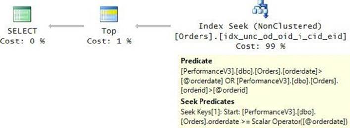
FIGURE 5-2 Plan for TOP with multiple anchor sort keys, first predicate form.
Observe that the Start property of the Seek Predicates property is based only on the predicate orderdate >= @orderdate. The residual predicate is orderdate > @orderdate OR orderid > @orderid. Such optimization could result in some unnecessary work scanning the pages holding the first part of the range with the first qualifying order date with the nonqualifying order IDs—in other words, the rows where orderdate = @orderdate AND orderid <= @orderid are going to be scanned even though they need not be returned. How many unnecessary page reads will be performed mainly depends on the density of the leading sort key—orderdate, in our case. The denser it is, the more unnecessary work is likely going to happen. In our case, the density of the orderdate column is very low (~1/1500); it is so low that the extra work is negligible. But, when the leading sort key is dense, you could get a noticeable improvement by using the second form of the predicate. Here’s an implementation of the stored procedure with the second predicate form:
IF OBJECT_ID(N'dbo.GetPage', N'P') IS NOT NULL DROP PROC dbo.GetPage;
GO
CREATE PROC dbo.GetPage
@orderdate AS DATE = '00010101', -- anchor sort key 1 (orderdate)
@orderid AS INT = 0, -- anchor sort key 2 (orderid)
@pagesize AS BIGINT = 25
AS
SELECT TOP (@pagesize) orderid, orderdate, custid, empid
FROM dbo.Orders
WHERE (orderdate = @orderdate AND orderid > @orderid)
OR orderdate > @orderdate
ORDER BY orderdate, orderid;
GO
Run the following code to get the third page:
EXEC dbo.GetPage @orderdate = '20101209', @orderid = 2830, @pagesize = 25;
The query plan for the implementation with the second form of the predicate is shown in Figure 5-3.
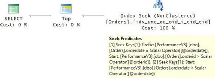
FIGURE 5-3 Plan for TOP with multiple anchor sort keys, second predicate form.
Observe that there’s no residual predicate, only Seek Predicates. Curiously, there are two seek predicates. Remember that, generally, the range scan performed by an Index Seek operator starts with the first match for Prefix and Start and ends with the last match for Prefix. In our case, one predicate (marked in the plan as [1] Seek Keys...) starts with orderdate = @orderdate AND orderid > @orderid and ends with orderdate = @orderdate. Another predicate (marked in the plan as [2] Seek Keys...) starts with orderdate = @orderdate and has no explicit end. What’s interesting is that during query execution, if Top Expression rows are found by the first seek, the execution of the operator short-circuits before getting to the second. But if the first seek isn’t sufficient, the second will be executed. The fact that in our example the leading sort key (orderdate) has low density could mislead you to think that the first predicate form is more efficient. If you test both implementations and compare the number of logical reads, you might see the first one performing 3 or more reads and the second one performing 6 or more reads (when two seeks are used). But if you test the solutions with a dense leading sort key, you will notice a significant difference in favor of the second solution.
There’s another method to using TOP to implement paging. You can think of it as the TOP over TOP, or nested TOP, method. You work with @pagenum and @pagesize as the inputs to the GetPage procedure. There’s no anchor concept here. You use one query with TOP to filter@pagenum * @pagesize rows based on the desired order. You define a table expression based on this query (call it D1). You use a second query against D1 with TOP to filter @pagesize rows, but in inverse order. You define a table expression based on the second query (call it D2). Finally, you write an outer query against D2 to order the rows in the desired order. Run the following code to implement the GetPage procedure based on this approach:
IF OBJECT_ID(N'dbo.GetPage', N'P') IS NOT NULL DROP PROC dbo.GetPage;
GO
CREATE PROC dbo.GetPage
@pagenum AS BIGINT = 1,
@pagesize AS BIGINT = 25
AS
SELECT orderid, orderdate, custid, empid
FROM ( SELECT TOP (@pagesize) *
FROM ( SELECT TOP (@pagenum * @pagesize) *
FROM dbo.Orders
ORDER BY orderid ) AS D1
ORDER BY orderid DESC ) AS D2
ORDER BY orderid;
GO
Here are three consecutive calls to the procedure requesting the first, second, and third pages:
EXEC dbo.GetPage @pagenum = 1, @pagesize = 25;
EXEC dbo.GetPage @pagenum = 2, @pagesize = 25;
EXEC dbo.GetPage @pagenum = 3, @pagesize = 25;
The plan for the third procedure call is shown in Figure 5-4.
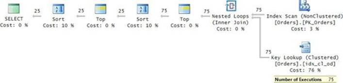
FIGURE 5-4 Plan for TOP over TOP.
The plan is not very expensive, but there are three aspects to it that are not optimal when compared to the implementation based on the anchor concept. First, the plan scans the data in the index from the beginning of the leaf until the last qualifying row. This means that there’s repetition of work—namely, rescanning portions of the data. For the first page requested by the user, the plan will scan 1 * @pagesize rows, for the second page it will scan 2 * @pagesize rows, for the nth page it will scan n * @pagesize rows. Second, notice that the Key Lookup operator is executed 75 times even though only 25 of the lookups are relevant. Third, there are two Sort operators added to the plan: one reversing the original order to get to the last chunk of rows, and the other reversing it back to the original order to present it like this. For the third page request, the execution of this plan performed 241 logical reads. The greater the number of pages you have, the more work there is.
The benefit of this approach compared to the anchor-based strategy is that you don’t need to deal with collecting the anchor from the result of the last page request, and the user is not limited to navigating only between adjacent pages. For example, the user can start with page 1, request page 5, and so on.
Optimization of OFFSET-FETCH
The optimization of the OFFSET-FETCH filter is similar to that of TOP. Instead of reinventing the wheel by creating an entirely new plan operator, Microsoft decided to enhance the existing Top operator. Remember the Top operator has a property called Top Expression that indicates how many rows to request from the operator to the right and pass to the operator to the left. The enhanced Top operator used to process OFFSET-FETCH has a new property called OffsetExpression that indicates how many rows to request from the operator to the right and not pass to the operator to the left. The OffsetExpression property is processed before the Top Expression property, as you might have guessed.
To show you the optimization of the OFFSET-FETCH filter, I’ll use it in the implementation of the GetPage procedure:
IF OBJECT_ID(N'dbo.GetPage', N'P') IS NOT NULL DROP PROC dbo.GetPage;
GO
CREATE PROC dbo.GetPage
@pagenum AS BIGINT = 1,
@pagesize AS BIGINT = 25
AS
SELECT orderid, orderdate, custid, empid
FROM dbo.Orders
ORDER BY orderid
OFFSET (@pagenum - 1) * @pagesize ROWS FETCH NEXT @pagesize ROWS ONLY;
GO
As you can see, OFFSET-FETCH allows a simple and flexible solution that uses the @pagenum and @pagesize inputs. Use the following code to request the first three pages:
EXEC dbo.GetPage @pagenum = 1, @pagesize = 25;
EXEC dbo.GetPage @pagenum = 2, @pagesize = 25;
EXEC dbo.GetPage @pagenum = 3, @pagesize = 25;
![]() Note
Note
Remember that under the default isolation level Read Committed, data changes between procedure calls can affect the results you get, causing you to get the same row in different pages or skip some rows. For example, suppose that at point in time T1, you request page 1. You get the rows that according to the paging sort order are positioned 1 through 25. Before you request the next page, at point in time T2, someone adds a new row with a sort key that makes it the 20th row. At point in time T3, you request page 2. You get the rows that, in T1, were positioned 25 through 49 and not 26 through 50. This behavior could be awkward. If you want the entire sequence of page requests to interact with the same state of the data, you need to submit all requests from the same transaction running under the snapshot isolation level.
The plan for the third execution of the procedure is shown in Figure 5-5.
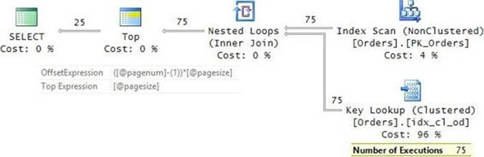
FIGURE 5-5 Plan for OFFSET-FETCH.
As you can see in the plan, the Top operator first requests OffsetExpression rows (50, in our example) from the operator to the right and doesn’t pass those to the operator to the left. Then it requests Top Expression rows (25, in our example) from the operator to the right and passes those to the operator to the left. You can see two levels of inefficiency in this plan compared to the plan for the anchor solution. One is that the Index Scan operator ends up scanning 75 rows, but only the last 25 are relevant. This is unavoidable without an input anchor to start after. But the Key Lookup operator is executed 75 times even though, theoretically, the first 50 times could have been avoided. Such logic to avoid applying lookups for the first OffsetExpression rows wasn’t added to the optimizer. The number of logical reads required for the third page request is 241. The farther away the page number you request is, the more lookups the plan applies and the more expensive it is.
Arguably, in paging sessions users don’t get too far. If users don’t find what they are looking for after the first few pages, they usually give up and refine their search. In such cases, the extra work is probably negligible enough to not be a concern. However, the farther you get with the page number you’re after, the more the inefficiency increases. For example, run the following code to request page 1000:
EXEC dbo.GetPage @pagenum = 1000, @pagesize = 25;
This time, the plan involves 25,000 lookups, resulting in a total number of logical reads of 76,644. Unfortunately, because the optimizer doesn’t have logic to avoid the unnecessary lookups, you need to figure this out yourself if it’s important for you to eliminate unnecessary costs. Fortunately, there is a simple trick you can use to achieve this. Have the query with the OFFSET-FETCH filter return only the sort keys. Define a table expression based on this query (call it K, for keys). Then in the outer query, join K with the underlying table to return all the remaining attributes you need. Here’s the optimized implementation of GetPage based on this strategy:
ALTER PROC dbo.GetPage
@pagenum AS BIGINT = 1,
@pagesize AS BIGINT = 25
AS
WITH K AS
(
SELECT orderid
FROM dbo.Orders
ORDER BY orderid
OFFSET (@pagenum - 1) * @pagesize ROWS FETCH NEXT @pagesize ROWS ONLY
)
SELECT O.orderid, O.orderdate, O.custid, O.empid
FROM dbo.Orders AS O
INNER JOIN K
ON O.orderid = K.orderid
ORDER BY O.orderid;
GO
Run the following code to get the third page:
EXEC dbo.GetPage @pagenum = 3, @pagesize = 25;
You will get the plan shown in Figure 5-6.
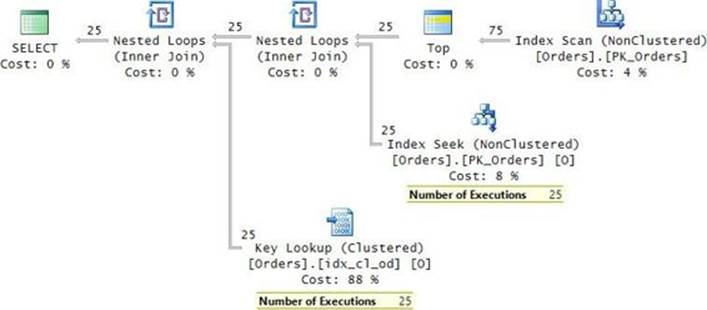
FIGURE 5-6 Plan for OFFSET-FETCH, minimizing lookups.
As you can see, the Top operator is used early in the plan to filter the relevant 25 keys. Then only 25 executions of the Index Seek operator are required, plus 25 executions of the Key Lookup operator (because PK_Orders is not a covering index). The total number of logical reads required for the processing of this plan for the third page request was reduced to 153. This doesn’t seem like a dramatic improvement when compared to the 241 logical reads used in the previous implementation. But try running the procedure with a page that’s farther out, like 1000:
EXEC dbo.GetPage @pagenum = 1000, @pagesize = 25;
The optimized implementation uses only 223 logical reads compared to the 76,644 used in the previous implementation. That’s a big difference!
Curiously, a noncovering index created only on the sort keys, like PK_Orders in our case, can be more efficient for the optimized solution than a covering index. That’s because with shorter rows, more rows fit in a page. So, in cases where you need to skip a substantial number of rows, you get to do so by scanning fewer pages than you would with a covering index. With a noncovering index, you do have the extra cost of the lookups, but the optimized solution reduces the number of lookups to the minimum.
OFFSET TO | AFTER
As food for thought, if you could change or extend the design of the OFFSET-FETCH filter, what would you do? You might find it useful to support an alternative OFFSET option that is based on an input-anchor sort vector. Imagine syntax such as the following (which shows additions to the standard syntax in bold):
OFFSET { <offset row count> { ROW | ROWS } | { TO | AFTER ( <sort vector> ) } }
FETCH { FIRST | NEXT } [ <fetch first quantity> ] { ROW | ROWS } { ONLY | WITH TIES }
[ LAST ROW INTO ( <variables vector> ) ]
You would then use a query such as the following in the GetPage procedure (but don’t try it, because it uses unsupported syntax):
SELECT orderid, orderdate, custid, empid
FROM dbo.Orders
ORDER BY orderdate, orderid
OFFSET AFTER (@anchor_orderdate, @anchor_orderid) -- input anchor sort keys
FETCH NEXT @pagesize ROWS ONLY
LAST ROW INTO (@last_orderdate, @last_orderid); -- outputs for next page request
The suggested anchor-based offset has a couple of advantages compared to the existing row count–based offset. The former lends itself to good optimization with an index seek directly to the first matching row in the leaf of a supporting index. Also, by using the former, you can see changes in the data gracefully, unlike with the latter.
Optimization of ROW_NUMBER
Another common solution for paging is using the ROW_NUMBER function to compute row numbers based on the desired sort and then filtering the right range of row numbers based on the input @pagenum and @pagesize.
Here’s the implementation of the GetPage procedure based on this strategy:
IF OBJECT_ID(N'dbo.GetPage', N'P') IS NOT NULL DROP PROC dbo.GetPage;
GO
CREATE PROC dbo.GetPage
@pagenum AS BIGINT = 1,
@pagesize AS BIGINT = 25
AS
WITH C AS
(
SELECT orderid, orderdate, custid, empid,
ROW_NUMBER() OVER(ORDER BY orderid) AS rn
FROM dbo.Orders
)
SELECT orderid, orderdate, custid, empid
FROM C
WHERE rn BETWEEN (@pagenum - 1) * @pagesize + 1 AND @pagenum * @pagesize
ORDER BY rn; -- if order by orderid get sort in plan
GO
Run the following code to request the first three pages:
EXEC dbo.GetPage @pagenum = 1, @pagesize = 25;
EXEC dbo.GetPage @pagenum = 2, @pagesize = 25;
EXEC dbo.GetPage @pagenum = 3, @pagesize = 25;
The plan for the third page request is shown in Figure 5-7.
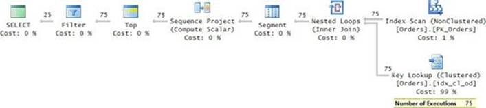
FIGURE 5-7 Plan for ROW_NUMBER.
Interestingly, the optimization of this solution is similar to that of the solution based on the OFFSET-FETCH filter. You will find the same inefficiencies, including the unnecessary lookups. As a result, the costs are virtually the same. For the third page request, the number of logical reads is 241. Run the procedure again asking for page 1000:
EXEC dbo.GetPage @pagenum = 1000, @pagesize = 25;
The number of logical reads is now 76,644. You can avoid the unnecessary lookups by applying the same optimization principle used in the improved OFFSET-FETCH solution, like so:
ALTER PROC dbo.GetPage
@pagenum AS BIGINT = 1,
@pagesize AS BIGINT = 25
AS
WITH C AS
(
SELECT orderid, ROW_NUMBER() OVER(ORDER BY orderid) AS rn
FROM dbo.Orders
),
K AS
(
SELECT orderid, rn
FROM C
WHERE rn BETWEEN (@pagenum - 1) * @pagesize + 1 AND @pagenum * @pagesize
)
SELECT O.orderid, O.orderdate, O.custid, O.empid
FROM dbo.Orders AS O
INNER JOIN K
ON O.orderid = K.orderid
ORDER BY K.rn;
GO
Run the procedure again requesting the third page:
EXEC dbo.GetPage @pagenum = 3, @pagesize = 25;
The plan for the optimized solution is shown in Figure 5-8.
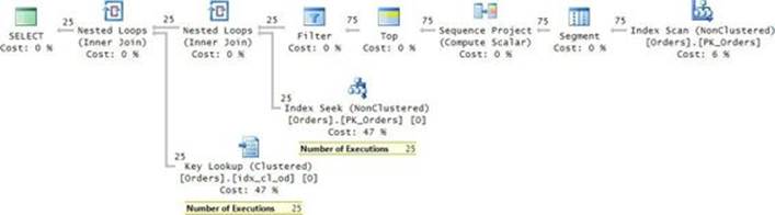
FIGURE 5-8 Plan for ROW_NUMBER, minimizing lookups.
Observe that the Top operator filters the first 75 rows, and then the Filter operator filters the last 25, before applying the seeks and the lookups. As a result, the seeks and lookups are executed only 25 times. The execution of the plan for the third page request involves 153 logical reads, compared to 241 required by the previous solution.
Run the procedure again, this time requesting page 1000:
EXEC dbo.GetPage @pagenum = 1000, @pagesize = 25;
This execution requires only 223 logical reads, compared to 76,644 required by the previous solution.
Using the TOP option with modifications
T-SQL supports using the TOP filter with modification statements. This section first describes this capability, and then its limitation and a workaround for the limitation. Then it describes a practical use case for this capability when you need to delete a large number of rows.
In my examples, I’ll use a table called MyOrders. Run the following code to create this table as an initial copy of the Orders table in the PerformanceV3 database:
USE PerformanceV3;
IF OBJECT_ID(N'dbo.MyOrders', N'U') IS NOT NULL DROP TABLE dbo.MyOrders;
GO
SELECT * INTO dbo.MyOrders FROM dbo.Orders;
CREATE UNIQUE CLUSTERED INDEX idx_od_oid ON dbo.MyOrders(orderdate, orderid);
TOP with modifications
With T-SQL, you can use TOP with modification statements. Those statements are INSERT TOP, DELETE TOP, UPDATE TOP, and MERGE TOP. This means the statement will stop modifying rows once the requested number of rows are affected. For example, the following statement deletes 50 rows from the table MyOrders:
DELETE TOP (50) FROM dbo.MyOrders;
When you use TOP in a SELECT statement, you can control which rows get chosen using the ORDER BY clause. But modification statements don’t have an ORDER BY clause. This means you can indicate how many rows you want to modify, but not based on what order—at least, not directly. So the preceding statement deletes 50 rows, but you cannot control which 50 rows get deleted. You should consider the order as being arbitrary. In practice, it depends on optimization and data layout.
This limitation is a result of the design choice that the TOP ordering is to be defined by the traditional ORDER BY clause. The traditional ORDER BY clause was originally designed to define presentation order, and it is available only to the SELECT statement. Had the design of TOP been different, with its own ordering specification that is not related to presentation ordering, it would have been natural to use also with modification statements. Here’s an example for what such a design might have looked like (but don’t run the code, because this syntax isn’t supported):
DELETE TOP (50) OVER(ORDER BY orderdate, orderid) FROM dbo.MyOrders;
Fortunately, when you do need to control which rows get chosen, you can use a simple trick as a workaround. Use a SELECT query with a TOP filter and an ORDER BY clause. Define a table expression based on that query. Then issue the modification against the table expression, like so:
WITH C AS
(
SELECT TOP (50) *
FROM dbo.MyOrders
ORDER BY orderdate, orderid
)
DELETE FROM C;
In practice, the rows from the underlying table will be affected. You can think of the modification as being defined through the table expression.
The OFFSET-FETCH filter is not supported directly with modification statements, but you can use a similar trick like the one with TOP.
Modifying in chunks
Having TOP supported by modification statements without the ability to indicate order might seem futile, but there is a practical use case involving modifying large volumes of data. As an example, suppose you need to delete all rows from the MyOrders table where the order date is before 2013. The table in our example is fairly small, having about 1,000,000 rows. But imagine there were 100,000,000 rows, and the number of rows to delete was about 50,000,000. If the table was partitioned (say, by year), things would be easy and highly efficient. You switch a partition out to a staging table and then drop the staging table. However, what if the table is currently not partitioned? The intuitive thing to do is to issue a simple DELETE statement to do the job as a single transaction, like so (but don’t run this statement):
DELETE FROM dbo.MyOrders WHERE orderdate < '20130101';
Such an approach can get you into trouble in a number of ways.
A DELETE statement is fully logged, unlike DROP TABLE and TRUNCATE TABLE statements. Log writes are sequential; therefore, log-intensive operations tend to be slow and hard to optimize beyond a certain point. For example, deleting 50,000,000 rows can take many minutes to finish.
There’s a section in the log considered to be the active portion, starting with the oldest open transaction and ending with the current pointer in the log. The active portion cannot be recycled. So when you have a long-running transaction, it can cause the transaction log to expand, sometimes well beyond its typical size for your database. This can be an issue if you have limited disk space.
Modification statements acquire exclusive locks on the modified resources (row or page locks, as decided by SQL Server dynamically), and exclusive locks are held until the transaction finishes. Each lock is represented by a memory structure that is approximately 100 bytes in size. Acquiring a large number of locks has two main drawbacks. For one, it requires large amounts of memory. Second, it takes time to allocate the memory structures, which adds to the time it takes the transaction to complete. To reduce the memory footprint and allow a faster process, SQL Server will attempt to escalate from the initial granularity of locks (row or page) to a table lock (or partition, if configured). The first trigger for SQL Server to attempt escalation is when the same transaction reaches 5,000 locks against the same object. If unsuccessful (for example, another transaction is holding locks that the escalated lock would be in conflict with), SQL Server will keep trying to escalate every additional 1,250 locks. When escalation succeeds, the transaction locks the entire table (or partition) until it finishes. This behavior can cause concurrency problems.
If you try to terminate such a large modification that is in progress, you will face the consequences of a rollback. If the transaction was already running for a while, it will take a while for the rollback to finish—typically, more than the original work.
To avoid the aforementioned problems, the recommended approach to apply a large modification is to do it in chunks. For our purge process, you can run a loop that executes a DELETE TOP statement repeatedly until all qualifying rows are deleted. You want to make sure that the chunk size is not too small so that the process will not take forever, but you want it to be small enough not to trigger lock escalation. The tricky part is figuring out the chunk size. It takes 5,000 locks before SQL Server attempts escalation, but how does this translate to the number of rows you’re deleting? SQL Server could decide to use row or page locks initially, plus when you delete rows from a table, SQL Server deletes rows from the indexes that are defined on the table. So it’s hard to predict what the ideal number of rows is without testing.
A simple solution could be to test different numbers while running a trace or an extended events session with a lock-escalation event. For example, I ran the following extended events session with a Live Data window open, while issuing DELETE TOP statements from a session with session ID 53:
CREATE EVENT SESSION [Lock_Escalation] ON SERVER
ADD EVENT sqlserver.lock_escalation(
WHERE ([sqlserver].[session_id]=(53)));
I started with 10,000 rows using the following statement:
DELETE TOP (10000) FROM dbo.MyOrders WHERE orderdate < '20130101';
Then I adjusted the number, increasing or decreasing it depending on whether an escalation event took place or not. In my case, the first point where escalation happened was somewhere between 6,050 and 6,100 rows. Once you find it, you don’t want to use that point minus 1. For example, if you add indexes later on, the point will become lower. To be on the safe side, I take the number that I find in my testing and divide it by two. This should leave enough room for the future addition of indexes. Of course, it’s worthwhile to retest from time to time to see if the number needs to be adjusted.
Once you have the chunk size determined (say, 3,000), you implement the purge process as a loop that deletes one chunk of rows at a time using a DELETE TOP statement, like so:
SET NOCOUNT ON;
WHILE 1 = 1
BEGIN
DELETE TOP (3000) FROM dbo.MyOrders WHERE orderdate < '20130101';
IF @@ROWCOUNT < 3000 BREAK;
END
The code uses an infinite loop. Every execution of the DELETE TOP statement deletes up to 3,000 rows and commits. As soon as the number of affected rows is lower than 3,000, you know that you’ve reached the last chunk, so the code breaks from the loop. If this process is running (and during peak hours), you want to abort it, and it’s quite safe to stop it. Only the current chunk will undergo a rollback. You can then run it again in the next window you have for this and the process will simply pick up where it left off.
Top N per group
The top N per group task is a classic task that appears in many shapes in practice. Examples include the following: “Return the latest price for each security,” “Return the employee who handled the most orders for each region,” “Return the three most recent orders for each customer,” and so on. Interestingly, like with many other examples in T-SQL, it’s not like there’s one solution that is considered the most efficient in all cases. Different solutions work best in different circumstances. For top N per group tasks, two main factors determine which solution is most efficient: the availability of a supporting index and the density of the partitioning (group) column.
The task I will use to demonstrate the different solutions is returning the three most recent orders for each customer from the Sales.Orders table in the TSQLV3 database. In any top N per group task, you need to identify the elements involved: partitioning, ordering, and covering. The partitioning element defines the groups. The ordering element defines the order—based on which, you filter the first N rows in each group. The covering element simply represents the rest of the columns you need to return. Here are the elements in our sample task:
![]() Partitioning: custid
Partitioning: custid
![]() Ordering: orderdate DESC, orderid DESC
Ordering: orderdate DESC, orderid DESC
![]() Covering: empid
Covering: empid
As mentioned, one of the important factors contributing to the efficiency of solutions is the availability of a supporting index. The recommended index is based on a pattern I like to think of as POC—the acronym for the elements involved (partitioning, ordering, and covering). The POelements should form the index key list, and the C element should form the index include list. If the index is clustered, only the key list is relevant; all the rest of the columns are included in the leaf row, anyway. Run the following code to create the POC index for our sample task:
USE TSQLV3;
CREATE UNIQUE INDEX idx_poc ON Sales.Orders(custid, orderdate DESC, orderid DESC)
INCLUDE(empid);
The other important factor in determining which solution is most efficient is the density of the partitioning element (custid, in our case). The Sales.Orders table in our example is very small, but imagine the same structure with a larger volume of data—say, 10,000,000 rows. The row size in our index is quite small (22 bytes), so over 300 rows fit in a page. This means the index will have about 30,000 pages in its leaf level and will be three levels deep. I’ll discuss two density scenarios in my examples:
![]() Low density: 1,000,000 customers, with 10 orders per customer on average
Low density: 1,000,000 customers, with 10 orders per customer on average
![]() High density: 10 customers, with 1,000,000 orders per customer on average
High density: 10 customers, with 1,000,000 orders per customer on average
I’ll start with a solution based on the ROW_NUMBER function that is the most efficient in the low-density case. I’ll continue with a solution based on TOP and APPLY that is the most efficient in the high-density case. Finally, I’ll describe a solution based on concatenation that performs better than the others when a POC index is not available, regardless of density.
Solution using ROW_NUMBER
Two main optimization strategies can be used to carry out our task. One strategy is to perform a seek for each customer in the POC index to the beginning of that customer’s section in the index leaf, and then perform a range scan of the three qualifying rows. Another strategy is to perform a single scan of the index leaf and then filter the interesting rows as part of the scan.
The former strategy is not efficient for low density because it involves a large number of seeks. For 1,000,000 customers, it requires 1,000,000 seeks. With three levels in the index, this approach translates to 3,000,000 random reads. Therefore, with low density, the strategy involving a single full scan and a filter is more efficient. From an I/O perspective, it should cost about 30,000 sequential reads.
To achieve the more efficient strategy for low density, you use the ROW_NUMBER function. You write a query that computes row numbers that are partitioned by custid and ordered by orderdate DESC, orderid DESC. This query is optimized with a single ordered scan of the POC index, as desired. You then define a CTE based on this query and, in the outer query, filter the rows with a row number that is less than or equal to 3. This part adds a Filter operator to the plan. Here’s the complete solution:
WITH C AS
(
SELECT
ROW_NUMBER() OVER(
PARTITION BY custid
ORDER BY orderdate DESC, orderid DESC) AS rownum,
orderid, orderdate, custid, empid
FROM Sales.Orders
)
SELECT custid, orderdate, orderid, empid
FROM C
WHERE rownum <= 3;
The execution plan for this solution is shown in Figure 5-9.
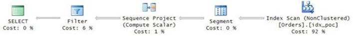
FIGURE 5-9 Plan for a solution with ROW_NUMBER.
As you can see, the majority of the cost of this plan is associated with the ordered scan of the POC index. As mentioned, if the table had 10,000,000 rows, the I/O cost would be about 30,000 sequential reads.
Solution using TOP and APPLY
If you have high density (10 customers, with 1,000,000 rows each), the strategy with the index scan is not the most efficient. With a small number of partitions (customers), a plan that performs a seek in the POC index for each partition is much more efficient.
If only a single customer is involved in the task, you can achieve a plan with a seek by using the TOP filter, like so:
SELECT TOP (3) orderid, orderdate, empid
FROM Sales.Orders
WHERE custid = 1
ORDER BY orderdate DESC, orderid DESC;
To apply this logic to each customer, use the APPLY operator with the preceding query against the Customers table, like so:
SELECT C.custid, A.orderid, A.orderdate, A.empid
FROM Sales.Customers AS C
CROSS APPLY ( SELECT TOP (3) orderid, orderdate, empid
FROM Sales.Orders AS O
WHERE O.custid = C.custid
ORDER BY orderdate DESC, orderid DESC ) AS A;
The execution plan for this solution is shown in Figure 5-10.
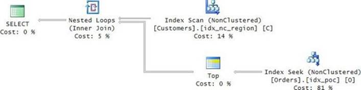
FIGURE 5-10 Plan for a solution with TOP and APPLY.
You get the desired plan for high density. With only 10 customers, this plan requires about 30 logical reads. That’s big savings compared to the cost of the scan strategy, which is 30,000 reads.
TOP OVER
Again, as a thought exercise, if you could change or extend the design of the TOP filter, what would you do? In the existing design, the ordering specification for TOP is based on the underlying query’s ORDER BY clause. An alternative design is for TOP to use its own ordering specification that is separate from the underlying query’s ORDER BY clause. This way, it is clear that the TOP ordering doesn’t provide any presentation-ordering guarantees, plus it would allow you to use a different ordering specification for the TOP filter and for presentation purposes. Furthermore, the TOP syntax could benefit from a partitioning element, in that the filter is applied per partition. Because the OVER clause used with window functions already supports partitioning and ordering specifications, there’s no need to reinvent the wheel. A similar syntax can be used with TOP, like so:
TOP ( < expression > ) [ PERCENT ] [ WITH TIES ]
[ OVER( [ PARTITION BY ( < partition by list > ) ] [ ORDER BY ( <order by list> ) ] ) ]
You then use the following query to request the three most recent orders for each customer (but do not run this query, because it relies on unsupported syntax):
SELECT TOP (3) OVER ( PARTITION BY custid ORDER BY orderdate, orderid )
orderid, orderdate, custid, empid
FROM dbo.Orders
ORDER BY custid, orderdate, orderid;
You can find a request to Microsoft to improve the TOP filter as described here in the following link: http://connect.microsoft.com/SQLServer/feedback/details/254390/over-clause-enhancement-request-top-over. Implementing such a design in SQL Server shouldn’t cause compatibility issues. SQL Server could assume the original behavior when an OVER clause isn’t present and the new behavior when it is.
Solution using concatenation (a carry-along sort)
Absent a POC index, both solutions I just described become inefficient and have problems scaling. The solution based on the ROW_NUMBER function will require sorting. Sorting has n log n scaling, becoming more expensive per row as the number of rows increases. The solution with the TOP filter and the APPLY operator might require an Index Spool operator (which involves the creation of an index during the plan) and sorting.
Interestingly, when N equals 1 in the top N per group task and a POC index is absent, there’s a third solution that performs and scales better than the other two.
Make sure you drop the POC index before proceeding:
DROP INDEX idx_poc ON Sales.Orders;
The third solution is based on the concatenation of elements. It implements a technique you can think of as a carry-along sort. You start by writing a grouped query that groups the rows by the P element (custid). In the SELECT list, you convert the O (orderdate DESC, orderid DESC) and C (empid) elements to strings and concatenate them into one string. What’s important here is to convert the original values into string forms that preserve the original ordering behavior of the values. For example, use leading zeros for integers, use the form YYYYMMDD for dates, and so on. It’s only important to preserve ordering behavior for the O element to filter the right rows. The C element should be added just to return it in the output. You apply the MAX aggregate to the concatenated string. This results in returning one row per customer, with a concatenated string holding the elements from the most recent order. Finally, you define a CTE based on the grouped query, and in the outer query you extract the individual columns from the concatenated string and convert them back to the original types. Here’s the complete solution query:
WITH C AS
(
SELECT
custid,
MAX( (CONVERT(CHAR(8), orderdate, 112)
+ RIGHT('000000000' + CAST(orderid AS VARCHAR(10)), 10)
+ CAST(empid AS CHAR(10)) ) COLLATE Latin1_General_BIN2 ) AS s
FROM Sales.Orders
GROUP BY custid
)
SELECT custid,
CAST( SUBSTRING(s, 1, 8) AS DATE ) AS orderdate,
CAST( SUBSTRING(s, 9, 10) AS INT ) AS orderid,
CAST( SUBSTRING(s, 19, 10) AS CHAR(10) ) AS empid
FROM C;
What’s nice about this solution is that it scales much better than the others. With a small input table, the optimizer usually sorts the data and then uses an order-based aggregate (the Stream Aggregate operator). But with a large input table, the optimizer usually uses parallelism, with a local hash-based aggregate for each thread doing the bulk of the work, and a global aggregate that aggregates the local ones. You can see this approach by running the carry-along-sort solution against the Orders table in the PerformanceV3 database:
USE PerformanceV3;
WITH C AS
(
SELECT
custid,
MAX( (CONVERT(CHAR(8), orderdate, 112)
+ RIGHT('000000000' + CAST(orderid AS VARCHAR(10)), 10)
+ CAST(empid AS CHAR(10)) ) COLLATE Latin1_General_BIN2 ) AS s
FROM dbo.Orders
GROUP BY custid
)
SELECT custid,
CAST( SUBSTRING(s, 1, 8) AS DATE ) AS orderdate,
CAST( SUBSTRING(s, 9, 10) AS INT ) AS orderid,
CAST( SUBSTRING(s, 19, 10) AS CHAR(10) ) AS empid
FROM C;
The execution plan for this query is shown in Figure 5-11.
![]()
FIGURE 5-11 Plan for a solution using concatenation.
This exercise emphasizes again that there are usually multiple ways to solve any given querying task, and it’s not like one of the solutions is optimal in all cases. In query tuning, different factors are at play, and under different conditions different solutions are optimal.
Median
Given a set of values, the median is the value below which 50 percent of the values fall. In other words, median is the 50th percentile. Median is such a classic calculation in the statistical analysis of data that many T-SQL solutions were created for it over time. I will focus on three solutions. The first uses the PERCENTILE_CONT window function. The second uses the ROW_NUMBER function. The third uses the OFFSET-FETCH filter and the APPLY operator.
Our calculation of median will be based on the continuous-distribution model. What this translates to is that when you have an odd number of elements involved, you should return the middle element. When you have an even number, you should return the average of the two middle elements. The alternative to the continuous model is the discrete model, which requires the returned value to be an existing value in the input set.
In my examples, I’ll use a table called T1 with groups represented by a column called grp and values represented by a column called val. You’re supposed to compute the median value for each group. The optimal index for median solutions is one defined on (grp, val) as the key elements. Use the following code to create the table and fill it with a small set of sample data to verify the validity of the solutions:
USE tempdb;
IF OBJECT_ID(N'dbo.T1', N'U') IS NOT NULL DROP TABLE dbo.T1;
GO
CREATE TABLE dbo.T1
(
id INT NOT NULL IDENTITY
CONSTRAINT PK_T1 PRIMARY KEY,
grp INT NOT NULL,
val INT NOT NULL
);
CREATE INDEX idx_grp_val ON dbo.T1(grp, val);
INSERT INTO dbo.T1(grp, val)
VALUES(1, 30),(1, 10),(1, 100),
(2, 65),(2, 60),(2, 65),(2, 10);
Use the following code to populate the table with a large set of sample data (10 groups, with 1,000,000 rows each) to check the performance of the solutions:
DECLARE
@numgroups AS INT = 10,
@rowspergroup AS INT = 1000000;
TRUNCATE TABLE dbo.T1;
DROP INDEX idx_grp_val ON dbo.T1;
INSERT INTO dbo.T1 WITH(TABLOCK) (grp, val)
SELECT G.n, ABS(CHECKSUM(NEWID())) % 10000000
FROM TSQLV3.dbo.GetNums(1, @numgroups) AS G
CROSS JOIN TSQLV3.dbo.GetNums(1, @rowspergroup) AS R;
CREATE INDEX idx_grp_val ON dbo.T1(grp, val);
Solution using PERCENTILE_CONT
Starting with SQL Server 2012, T-SQL supports window functions to compute percentiles. PERCENTILE_CONT implements the continuous model, and PERCENTILE_DISC implements the discrete model. The functions are not implemented as grouped, ordered set functions; rather, they are implemented as window functions. This means that instead of grouping the rows by the grp column, you will define the window partition based on grp. Consequently, the function will return the same result for all rows in the same partition instead of once per group. To get the result only once per group, you need to apply the DISTINCT option. Here’s the solution to compute median using the continuous model with PERCENTILE_CONT:
SELECT
DISTINCT grp, PERCENTILE_CONT(0.5) WITHIN GROUP(ORDER BY val) OVER(PARTITION BY grp) AS median
FROM dbo.T1;
After you overcome the awkwardness in using a window function instead of a grouped one, you might find the solution agreeable because of its simplicity and brevity. That’s until you actually run it and look at its execution plan (which is not for the faint of heart). The plan for the solution is very long and inefficient. It does two rounds of spooling the data in work tables, reading each spool twice—once to get the detail and once to compute aggregates. It took the solution 79 seconds to complete in my system against the big set of sample data. If good performance is important to you, you should consider other solutions.
Solution using ROW_NUMBER
The second solution defines two CTEs. One called Counts is based on a grouped query that computes the count (column cnt) of rows per group. Another is called RowNums, and it computes row numbers (column n) for the detail rows. The outer query joins Counts with RowNums, and it filters only the relevant values for the median calculation. (Keep in mind that that the relevant values are those where n is (cnt+1)/2 or (cnt+2)/2, using integer division.) Finally, the outer query groups the remaining rows by the grp column and computes the average of the val column as the median. Here’s the complete solution:
WITH Counts AS
(
SELECT grp, COUNT(*) AS cnt
FROM dbo.T1
GROUP BY grp
),
RowNums AS
(
SELECT grp, val,
ROW_NUMBER() OVER(PARTITION BY grp ORDER BY val) AS n
FROM dbo.T1
)
SELECT C.grp, AVG(1. * R.val) AS median
FROM Counts AS C
INNER MERGE JOIN RowNums AS R
on C.grp = R.grp
WHERE R.n IN ( ( C.cnt + 1 ) / 2, ( C.cnt + 2 ) / 2 )
GROUP BY C.grp;
The plan for this solution is shown in Figure 5-12.
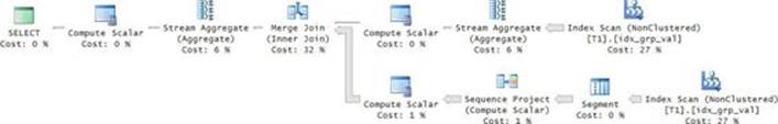
FIGURE 5-12 Plan for a solution using ROW_NUMBER.
SQL Server chose a serial plan that performs two scans of the index, a couple of order-based aggregates, a computation of row numbers, and a merge join. Compared to the previous solution with the PERCENTILE_CONT function, the new solution is quite efficient. It took only 8 seconds to complete in my system. Still, perhaps there’s room for further improvements. For example, you could try to come up with a solution that uses a parallel plan, you could try to reduce the number of pages that need to be scanned, and you could try to eliminate the fairly expensive merge join.
Solution using OFFSET-FETCH and APPLY
The third solution I’ll present uses the APPLY operator and the OFFSET-FETCH filter. The solution defines a CTE called C, which is based on a grouped query that computes for each group parameters for the OFFSET and FETCH clauses based on the group count. The offset value (call itov) is computed as (count – 1) / 2, and the fetch value (call it fv) is computed as 2 – count % 2. For example, if you have a group with 11 rows, ov is 5 and fv is 1. For a group with 12 rows, ov is 5 and fv is 2. The outer query applies to each group in C an OFFSET-FETCH query that retrieves the relevant values. Finally, the outer query groups the remaining rows and computes the average of the values as the median.
WITH C AS
(
SELECT grp,
COUNT(*) AS cnt,
(COUNT(*) - 1) / 2 AS ov,
2 - COUNT(*) % 2 AS fv
FROM dbo.T1
GROUP BY grp
)
SELECT grp, AVG(1. * val) AS median
FROM C
CROSS APPLY ( SELECT O.val
FROM dbo.T1 AS O
where O.grp = C.grp
order by O.val
OFFSET C.ov ROWS FETCH NEXT C.fv ROWS ONLY ) AS A
GROUP BY grp;
The plan for this solution is shown in Figure 5-13.
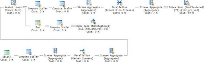
FIGURE 5-13 Plan for a solution using OFFSET-FETCH and APPLY.
The plan for the third solution has three advantages over the plan for the second. One is that it uses parallelism efficiently. The second is that the index is scanned in total one and a half times rather than two. The cost of the seeks is negligible here because the data has dense groups. The third advantage is that there’s no merge join in the plan. It took only 1 second for this solution to complete on my system. That’s quite impressive for 10,000,000 rows.
Conclusion
This chapter covered the TOP and OFFSET-FETCH filters. It started with a logical description of the filters. It then continued with optimization aspects demonstrated through paging solutions. You saw how critical it is to have an index on the sort columns to get good performance. Even with an index, I gave recommendations how to alter the solutions to avoid unnecessary lookups.
The chapter also covered modifying data with the TOP filter. Finally, the chapter concluded by demonstrating the use of TOP and OFFSET-FETCH to solve common tasks like top N per group and using a median value.