T-SQL Querying (2015)
Chapter 8. T-SQL for BI practitioners
Huge amounts of data already exist in transactional databases worldwide. There is more and more need to analyze this data. Database and business intelligence (BI) developers need to create thousands, if not millions, of reports on a daily basis. Many of these reports include statistical analyses. Statistical analysis of data is useful for data overview and data quality assessment, which are two typical initial stages of more in-depth analyses. However, there are not many statistical functions in Microsoft SQL Server. In addition, a good understanding of statistics is not common among T-SQL practitioners.
This chapter explains the basics of statistical analysis. It introduces many ways to calculate different statistics with T-SQL and Common Language Runtime (CLR) code. The code is based on real-life experience. I developed the code for myself because I am dealing with BI projects, especially with data mining, and I needed to create a lot of statistical queries in the initial state of many projects. Of course, there are many statistical packages available for purchase. However, many of my clients do not permit installing any additional software on their systems. Therefore, the only software I can rely upon is SQL Server.
Optimizing statistical queries is different than optimizing transactional queries. To calculate statistics, the query typically scans all the data. If the query is too slow, you can prepare a random sample of your data and then scan the sample data. However, if the queries follow the formulas blindly, many times they finish with multiple scans of the data. Optimizing such queries means minimizing the number of passes through the data. To achieve this task, you often need to develop an algorithm that uses additional mathematics to convert the formulas to equivalent ones that can be better optimized in SQL Server. You also need to understand T-SQL in depth. For example, you need a really good understanding of window functions and calculations. Besides teaching you about statistics and statistical queries, this chapter will help you with query optimization for efficiently writing nonstatistical queries too.
Data preparation
Before starting any statistical analysis, you need to understand what you are analyzing. In statistics, you analyze cases using their variables. To put it in SQL Server terminology, you can think of a case as a row in a table, and you can think of a variable as a column in the same table. For most statistical analyses, you prepare a single table or view. It is not always easy to define your case. For example, for a credit-risk analysis, you might define a family as a case, rather than defining it as a single customer. When you prepare the data for statistical analyses, you have to transform the source data accordingly. For each case, you need to encapsulate all available information in the columns of the table you are going to analyze.
Before starting a serious data overview, you need to understand how data values are measured in your data set. You might need to check this with a subject matter expert and analyze the business system that is the source for your data. There are different ways to measure data values and different types of columns:
![]() Discrete variables These variables can take a value only from a limited domain of possible values. Discrete values include categorical or nominal variables that have no natural order. Examples include states, status codes, and colors. Ranks can also take a value only from a discrete set of values. They have an order but do not permit any arithmetic. Examples include opinion ranks and binned (grouped, discretized) true numeric values.
Discrete variables These variables can take a value only from a limited domain of possible values. Discrete values include categorical or nominal variables that have no natural order. Examples include states, status codes, and colors. Ranks can also take a value only from a discrete set of values. They have an order but do not permit any arithmetic. Examples include opinion ranks and binned (grouped, discretized) true numeric values.
There are also some specific types of categorical variables. Single-valued variables, or constants, are not very interesting for analysis because they do not contribute any information. Two-valued, or dichotomous, variables have two values, which is the minimum needed for any analysis. Binary variables are specific dichotomous variables that take on only the values 0 and 1.
![]() Continuous variables These variables can take any of an unlimited number of possible values; however, the domain itself can have a lower boundary, upper boundary, or both. Intervals have one or two boundaries, have an order, and allow some arithmetic-like subtraction, but they do not always have a summation. Examples include dates, times, and temperatures. True numeric variables support all arithmetic. Examples include amounts and values. Monotonic variables are a specific type of continuous variables, which increase monotonously without bound. If they are simply IDs, they might not be interesting. Still, they can be transformed (binned into categories) if the ever-growing ID contains time order information (lower IDs are older than higher IDs).
Continuous variables These variables can take any of an unlimited number of possible values; however, the domain itself can have a lower boundary, upper boundary, or both. Intervals have one or two boundaries, have an order, and allow some arithmetic-like subtraction, but they do not always have a summation. Examples include dates, times, and temperatures. True numeric variables support all arithmetic. Examples include amounts and values. Monotonic variables are a specific type of continuous variables, which increase monotonously without bound. If they are simply IDs, they might not be interesting. Still, they can be transformed (binned into categories) if the ever-growing ID contains time order information (lower IDs are older than higher IDs).
Sales analysis view
In this chapter, I will perform all the statistical queries on a view for sales analysis. In this view, I join the OrderDetails table with the Orders, Customers, Products, Categories, and Employees tables to get some interesting variables to analyze. I am not using all the columns in the following code. However, you can use them for further investigation and tests of the statistical queries.
To create the SalesAnalysis view, run the code in Listing 8-1. Partial contents (a selection of columns and rows) of the SalesAnalysis view are shown in Table 8-1.
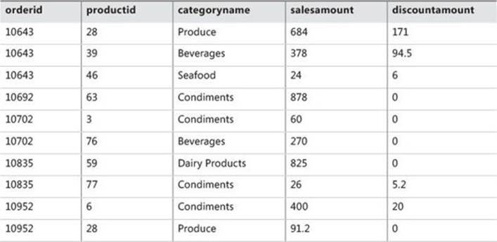
TABLE 8-1 Partial contents of the SalesAnalysis view
LISTING 8-1 Data-definition language for the SalesAnalysis view.
SET NOCOUNT ON;
USE TSQLV3;
IF OBJECT_ID(N'dbo.SalesAnalysis', N'V') IS NOT NULL DROP VIEW dbo.SalesAnalysis;
GO
CREATE VIEW dbo.SalesAnalysis
AS
SELECT O.orderid, P.productid, C.country AS customercountry,
CASE
WHEN c.country IN
(N'Argentina', N'Brazil', N'Canada', N'Mexico',
N'USA', N'Venezuela') THEN 'Americas'
ELSE 'Europe'
END AS 'customercontinent',
e.country AS employeecountry, PC.categoryname,
YEAR(O.orderdate) AS orderyear,
DATEDIFF(day, O.requireddate, o.shippeddate) AS requiredvsshipped,
OD.unitprice, OD.qty, OD.discount,
CAST(OD.unitprice * OD.qty AS NUMERIC(10,2)) AS salesamount,
CAST(OD.unitprice * OD.qty * OD.discount AS NUMERIC(10,2)) AS discountamount
FROM Sales.OrderDetails AS OD
INNER JOIN Sales.Orders AS O
ON OD.orderid = O.orderid
INNER JOIN Sales.Customers AS C
ON O.custid = C.custid
INNER JOIN Production.Products AS P
ON OD.productid = P.productid
INNER JOIN Production.Categories AS PC
ON P.categoryid = PC.categoryid
INNER JOIN HR.Employees AS E
ON O.empid = E.empid;
GO
Frequencies
For a quick overview of discrete variables, use frequency tables. In a frequency table, you can show values, absolute frequency of those values, absolute percentage, cumulative frequency, cumulative percentage, and the histogram of the absolute percentage.
Frequencies without window functions
Calculating the absolute frequency and absolute percentage is a straightforward aggregation. However, calculating the cumulative frequency and cumulative percentage means calculating running totals. Before SQL Server 2012 added support for window aggregate functions with a frame, you needed to use either correlated subqueries or non-equi self joins for this task. Both methods are pretty inefficient.
Run the following code to analyze the frequency distribution of the categoryname variable, which implements a solution with correlated subqueries:
WITH FreqCTE AS
(
SELECT categoryname,
COUNT(categoryname) AS absfreq,
ROUND(100. * (COUNT(categoryname)) /
(SELECT COUNT(*) FROM dbo.SalesAnalysis), 4) AS absperc
FROM dbo.SalesAnalysis
GROUP BY categoryname
)
SELECT C1.categoryname,
C1.absfreq,
(SELECT SUM(C2.absfreq)
FROM FreqCTE AS C2
WHERE C2.categoryname <= C1.categoryname) AS cumfreq,
CAST(ROUND(C1.absperc, 0) AS INT) AS absperc,
CAST(ROUND((SELECT SUM(C2.absperc)
FROM FreqCTE AS C2
WHERE C2.categoryname <= C1.categoryname), 0) AS INT) AS cumperc,
CAST(REPLICATE('*',C1.absPerc) AS VARCHAR(100)) AS histogram
FROM FreqCTE AS C1
ORDER BY C1.categoryname;
The preceding code generates the following output:
categoryname absfreq cumfreq absperc cumperc histogram
--------------- ----------- ----------- ----------- ----------- -------------------
Beverages 404 404 19 19 *******************
Condiments 216 620 10 29 **********
Confections 334 954 15 44 ***************
Dairy Products 366 1320 17 61 *****************
Grains/Cereals 196 1516 9 70 *********
Meat/Poultry 173 1689 8 78 ********
Produce 136 1825 6 84 ******
Seafood 330 2155 15 100 ***************
Frequencies with window functions
A much more efficient solution uses the window aggregate functions with a frame available in SQL Server versions 2012 and newer. The first part of the query, the common table expression query that calculates the absolute numbers, is the same as in the previous query. However, the cumulative values, also known as the running totals, are calculated with the help of the window aggregate functions.
WITH FreqCTE AS
(
SELECT categoryname,
COUNT(categoryname) AS absfreq,
ROUND(100. * (COUNT(categoryname)) /
(SELECT COUNT(*) FROM dbo.SalesAnalysis), 4) AS absperc
FROM dbo.SalesAnalysis
GROUP BY categoryname
)
SELECT categoryname,
absfreq,
SUM(absfreq)
OVER(ORDER BY categoryname
ROWS BETWEEN UNBOUNDED PRECEDING
AND CURRENT ROW) AS cumfreq,
CAST(ROUND(absperc, 0) AS INT) AS absperc,
CAST(ROUND(SUM(absperc)
OVER(ORDER BY categoryname
ROWS BETWEEN UNBOUNDED PRECEDING
AND CURRENT ROW), 0) AS INT) AS CumPerc,
CAST(REPLICATE('*',absperc) AS VARCHAR(50)) AS histogram
FROM FreqCTE
ORDER BY categoryname;
Of course, the output of this query is the same as the output of the previous query.
I found another interesting solution with window analytic functions. The CUME_DIST function calculates the cumulative distribution of a value in a group of values. That is, CUME_DIST computes the relative position of a specified value in a group of values. For a row r, assuming ascending ordering, the CUME_DIST of r is the number of rows with values lower than or equal to the value of r, divided by the number of rows evaluated in the partition or query result set. The PERCENT_RANK function calculates the relative rank of a row within a group of rows. Use PERCENT_RANK to evaluate the relative standing of a value within a query result set or partition.
The following query calculates the row number once partitioned over the categoryname column and once over the entire input set. It also calculates the percent rank and the cumulative distribution over the complete input set:
SELECT categoryname,
ROW_NUMBER() OVER(PARTITION BY categoryname
ORDER BY categoryname, orderid, productid) AS rn_absfreq,
ROW_NUMBER() OVER(
ORDER BY categoryname, orderid, productid) AS rn_cumfreq,
PERCENT_RANK()
OVER(ORDER BY categoryname) AS pr_absperc,
CUME_DIST()
OVER(ORDER BY categoryname, orderid, productid) AS cd_cumperc
FROM dbo.SalesAnalysis;
Partial output with rows is interesting for showing the algorithm for calculating frequencies:
categoryname rn_absfreq rn_cumfreq pr_absperc cd_cumperc
--------------- ---------- ---------- ---------------------- ----------------------
Beverages 1 1 0 0.000464037122969838
Beverages 2 2 0 0.000928074245939675
... ...
Beverages 404 404 0 0.187470997679814
Condiments 1 405 0.187558031569174 0.187935034802784
... ...
Condiments 216 620 0.187558031569174 0.287703016241299
Confections 1 621 0.287836583101207 0.288167053364269
As you can see, the last row number in a category actually represents the absolute frequency of the values in that category. The last unpartitioned row number in a category represents the cumulative frequency up to and including the current category. For example, the absolute frequency for beverages is 404 and the cumulative frequency is 404; for condiments, the absolute frequency is 216 and the cumulative frequency is 620. The CUME_DIST function (the cd_cumperc column in the output) for the last row in a category returns the cumulative percentage up to and including the category. If you subtract the PERCENT_RANK (the pr_absperc column in the output) for the last row in a category from the CUME_DIST of the last row in a category, you get the absolute percentage for the category. For example, the absolute percentage for condiments is around 10 percent (0.287703016241299 – 0.187558031569174).
The following query calculates the frequency distribution using the observations from the results of the previous query:
WITH FreqCTE AS
(
SELECT categoryname,
ROW_NUMBER() OVER(PARTITION BY categoryname
ORDER BY categoryname, orderid, productid) AS rn_absfreq,
ROW_NUMBER() OVER(
ORDER BY categoryname, orderid, productid) AS rn_cumfreq,
ROUND(100 * PERCENT_RANK()
OVER(ORDER BY categoryname), 4) AS pr_absperc,
ROUND(100 * CUME_DIST()
OVER(ORDER BY categoryname, orderid, productid), 4) AS cd_cumperc
FROM dbo.SalesAnalysis
)
SELECT categoryname,
MAX(rn_absfreq) AS absfreq,
MAX(rn_cumfreq) AS cumfreq,
ROUND(MAX(cd_cumperc) - MAX(pr_absperc), 0) AS absperc,
ROUND(MAX(cd_cumperc), 0) AS cumperc,
CAST(REPLICATE('*',ROUND(MAX(cd_cumperc) - MAX(pr_absperc),0)) AS VARCHAR(100)) AS histogram
FROM FreqCTE
GROUP BY categoryname
ORDER BY categoryname;
GO
Although the concept of the last query is interesting, it is not as efficient as one using the window aggregate function. Therefore, the second query from these three solutions for calculating the frequency distribution is the recommended one.
Descriptive statistics for continuous variables
Frequencies are useful for analyzing the distribution of discrete variables. You describe continuous variables with population moments, which are measures that give you some insight into the distribution. These measures give you an insight into the distribution of the values of the continuous variables. The first four population moments include center, spread, skewness, and peakedness of a distribution.
Centers of a distribution
There are many measures for a center of a distribution. Here are three of the most popular ones:
![]() The mode is the most frequent (that is, the most popular) value. This is the number that appears most often in a set of numbers. It is not necessarily unique—a distribution can have the same maximum frequency at different values.
The mode is the most frequent (that is, the most popular) value. This is the number that appears most often in a set of numbers. It is not necessarily unique—a distribution can have the same maximum frequency at different values.
![]() The median is the middle value in your distribution. When the number of cases is odd, the median is the middle entry in the data after you sort your variable data points in increasing order. When the number of cases is even, the median is equal to the sum of the two middle numbers (sorted in increasing order) divided by two. Note that there are other definitions of median, as I will show with the T-SQL PERCENTILE_CONT and PERCENTILE_DISC functions.
The median is the middle value in your distribution. When the number of cases is odd, the median is the middle entry in the data after you sort your variable data points in increasing order. When the number of cases is even, the median is equal to the sum of the two middle numbers (sorted in increasing order) divided by two. Note that there are other definitions of median, as I will show with the T-SQL PERCENTILE_CONT and PERCENTILE_DISC functions.
![]() The mean is the average value of your distribution. This is actually the arithmetic mean. There are other types of means, such as a geometric mean or harmonic mean. To avoid confusion, you should use the term arithmetic mean. However, for the sake of simplicity, I will use the termmean in the following text when discussing the arithmetic mean.
The mean is the average value of your distribution. This is actually the arithmetic mean. There are other types of means, such as a geometric mean or harmonic mean. To avoid confusion, you should use the term arithmetic mean. However, for the sake of simplicity, I will use the termmean in the following text when discussing the arithmetic mean.
You’ll find it useful to calculate more than one measure—more than one center of a distribution. You get some idea of the distribution just by comparing the values of the mode, median, and mean. If the distribution is symmetrical and has only a single peak, the mode, median, and mean all coincide. If not, the distribution is skewed in some way. Perhaps it has a long tail to the right. Then the mode would stay on the value with the highest relative frequency, while the median would move to the right to pick up half the observations. Half of the observations lie on either side of the median, but the cases on the right are farther out and exert more downward leverage. To balance them out, the mean must move even further to the right. If the distribution of data is skewed to the left, the mean is less than the median, which is often less than the mode. If the distribution of data is skewed to the right, the mode is often less than the median, which is less than the mean. However, calculating how much the distribution is skewed means calculating the third population moment, the skewness, which is explained later in this chapter.
Mode
The mode is the most fashionable value of a distribution—mode is actually the French word for fashion. Calculating the mode is simple and straightforward. In the following query, I use the TOP (1) WITH TIES expression to get the most frequent values in the distribution of the salesamountvariable.
SELECT TOP (1) WITH TIES salesamount, COUNT(*) AS number
FROM dbo.SalesAnalysis
GROUP BY salesamount
ORDER BY COUNT(*) DESC;
The result is
salesamount number
--------------------------------------- -----------
360.00 29
The WITH TIES clause is needed because there could be more than one value with the same number of occurrences in the distribution. We call distributions with more than one mode bi-modal distribution, three-modal distribution, and so on.
Median
The median is the value that splits the distribution into two halves. The number of rows with a value lower than the median must be equal to the number of rows with a value greater than the median for a selected variable. If there is an odd number of rows, the median is the middle row. If the number of rows is even, the median can be defined as the average value of the two middle rows (the financial median), the smaller of them (the lower statistical median), or the larger of them (the upper statistical median).
The PERCENTILE_DISC function computes a specific percentile for sorted values in an entire rowset or within distinct partitions of a rowset. For a given percentile value P, PERCENTILE_DISC sorts the values of the expression in the ORDER BY clause and returns the value with the smallest CUME_DIST value (with respect to the same sort specification) that is greater than or equal to P. PERCENTILE_DISC calculates the percentile based on a discrete distribution of the column values; the result is equal to a specific value in the column. Therefore, the PERCENTILE_DISC (0.5) function calculates the lower statistical median.
The PERCENTILE_CONT function calculates a percentile based on a continuous distribution of the column value in SQL Server. The result is interpolated and might not be equal to any specific values in the column. Therefore, this function calculates the financial median. The financial median is by far the most-used median.
The following code shows the difference between the PERCENTILE_DISC and PERCENTILE_CONT functions. It creates a simple table and inserts four rows with the values 1, 2, 3, and 4 for the only column in the table. Then it calculates the lower statistical and financial medians:
IF OBJECT_ID(N'dbo.TestMedian',N'U') IS NOT NULL
DROP TABLE dbo.TestMedian;
GO
CREATE TABLE dbo.TestMedian
(
val INT NOT NULL
);
GO
INSERT INTO dbo.TestMedian (val)
VALUES (1), (2), (3), (4);
SELECT DISTINCT -- can also use TOP (1)
PERCENTILE_DISC(0.5) WITHIN GROUP (ORDER BY val) OVER () AS mediandisc,
PERCENTILE_CONT(0.5) WITHIN GROUP (ORDER BY val) OVER () AS mediancont
FROM dbo.TestMedian;
GO
The result of the code is
mediandisc mediancont
----------- ----------------------
2 2.5
You can clearly see the difference between the two percentile functions. I calculate the financial median for the salesamount column of the SalesAnalysis view in the following query:
SELECT DISTINCT
PERCENTILE_CONT(0.5) WITHIN GROUP (ORDER BY salesamount) OVER () AS median
FROM dbo.SalesAnalysis;
The query returns the following result:
median
----------------------
360
In this case, for the salesamount column, the mode and the median are equal. However, this does not mean that the distribution is not skewed. I need to calculate the mean as well before making any conclusion about the skewness.
Mean
The mean is the most common measure for determining the center of a distribution. It is also probably the most abused statistical measure. The mean does not mean anything without the standard deviation (explained later in the chapter), and it should never be used alone. Let me give you an example. Imagine there are two pairs of people. In the first pair, both people earn the same wage—let’s say, $80,000 per year. In the second pair, one person earns $30,000 per year, while the other earns $270,000 per year. The mean wage for the first pair is $80,000, while the mean for the second pair is $150,000 per year. By just listing the mean, you could conclude that each person from the second pair earns more than either of the people in the first pair. However, you can clearly see that this would be a seriously incorrect conclusion.
The definition of the mean is simple: it is the sum of all values of a continuous variable divided by the number of cases, as shown in the following formula:
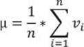
Because of the great importance of the mean, the T-SQL language has included the AVG aggregate function. The following query uses it to calculate the mean value for the salesamount variable:
SELECT AVG(salesamount) AS mean
FROM dbo.SalesAnalysis;
The result of the query is
mean
-----------
628.519067
Compare this value to the value for the median and the mode, which is 360. Apparently, the mean is much higher; this means that the distribution is skewed to the right, having a long tail of infrequent, but high values on the right side—that is, on the side with bigger values.
The mean is the first population moment. It is also called the estimated value or the estimator, because you can use it to estimate the value of a variable for an unknown case. However, you have already seen that the mean alone can be a very bad estimator.
Spread of a distribution
As mentioned, you need to know how spread out or varied the observations are—are you dealing with a very uniform or a very spread population? Similar to the center, the spread can be measured in several ways as well.
From among the many different definitions for the spread of the distribution, I will discuss the most popular ones: the range, the inter-quartile range, the mean absolute and mean squared deviation, the variance, and the standard deviation. I will also introduce the term degrees of freedomand explain the difference between variance and standard deviation for samples and for population.
Range
The range is the simplest measure of the spread; it is the plain distance between the maximal value and the minimal value that the variable takes. (A quick review: a variable is an attribute of an observation, represented as a column in a table.) The first formula for the range is
R = vmax – vmin
Of course, you use the MAX and MIN T-SQL aggregate functions to calculate the range of a variable:
SELECT MAX(salesamount) - MIN(salesamount) AS range
FROM dbo.SalesAnalysis;
You get the following output:
range
-----------
15805.20
Inter-Quartile range
The median is the value that splits the distribution into two halves. You can split the distribution more—for example, you can split each half into two halves. This way, you get quartiles as three values that split the distribution into quarters. Let’s generalize this splitting process. You start with sorting rows (cases, observations) on a selected column (attribute, variable). You define the rank as the absolute position of a row in your sequence of sorted rows. The percentile rank of a value is a relative measure that tells you how many percent of all (n) observations have a lower value than the selected value.
By splitting the observations into quarters, you get three percentiles (at 25%, 50%, and 75% of all rows), and you can read the values at those positions that are important enough to have their own names: the quartiles. The second quartile is, of course, the median. The first one is called thelower quartile and the third one is known as the upper quartile. If you subtract the lower quartile (the first one) from the upper quartile (the third one), you get the formula for the Inter-Quartile Range (IQR):
IQR = Q3 – Q1
Calculating the IQR is simple with the window analytic function PERCENTILE_CONT:
SELECT DISTINCT
PERCENTILE_CONT(0.75) WITHIN GROUP (ORDER BY salesamount) OVER () -
PERCENTILE_CONT(0.25) WITHIN GROUP (ORDER BY salesamount) OVER () AS IQR
FROM dbo.SalesAnalysis;
This query returns the following result:
IQR
---------
568.25
The IQR is resistant to a change just like the median. This means it is not sensitive to a wild swing in a single observation. (Let’s quickly review: a single observation is a single case, represented as a row in a table.) The resistance is logical, because you use only two key observations. When you see a big difference between the range and the inter-quartile range of the same variable, like in the salesamount variable in the example, some values in the distribution are quite far away from the mean value.
Mean absolute deviation
For the IQR, you use only two key observations: the lower and upper quartiles. Is there a measure that would take both observations into account? You can measure the distance between each value and the mean value and call it the deviation. The sum of all distances gives you a measure of how spread out your population is. But you must consider that some of the distances are positive while others are negative; actually, they mutually cancel themselves out, so the total gives you exactly zero. The same is true for the average of the deviations, so this would be a useless measure of spread. You solve this problem by ignoring the signs, and instead using the absolute values of the distances. Calculating the average of the absolute deviations, you get the formula for the Mean Absolute Deviation (MAD):
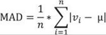
From the formula for the MAD, you can see that you need to calculate the mean with the AVG T-SQL aggregate function and then use this aggregation in the SUM T-SQL aggregate function. However, SQL Server cannot perform an aggregate function on an expression containing an aggregate or a subquery; therefore, I am going to do it by storing the mean value to a variable:
DECLARE @mean AS NUMERIC(10,2);
SET @mean = (SELECT AVG(salesamount) FROM dbo.SalesAnalysis);
SELECT SUM(ABS(salesamount - @mean))/COUNT(*) AS MAD
FROM dbo.SalesAnalysis;
You get the following output:
MAD
---------------------------------------
527.048886
Mean squared deviation
Another way of avoiding the problems of the signs of the deviations is to square each deviation. With a slight modification of the MAD formula—specifically, calculating the average of the squared deviations instead of the absolute deviations—you get the formula for the Mean Squared Deviation (MSD):
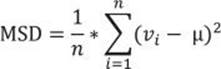
To calculate the MSD, you need to change the query for the MAD slightly:
DECLARE @mean AS NUMERIC(10,2);
SET @mean = (SELECT AVG(salesamount) FROM dbo.SalesAnalysis);
SELECT SUM(SQUARE(salesamount - @mean))/COUNT(*) AS MSD
FROM dbo.SalesAnalysis;
The query returns the following result for the MSD:
MSD
----------------------
1073765.30181991
Degrees of freedom and variance
Let’s suppose for a moment you have only one observation (n=1). This observation is also your sample mean, but there is no spread at all. You can calculate the spread only if you have the n that exceeds 1. Only the (n–1) pieces of information help you calculate the spread, considering that the first observation is your mean. These pieces of information are called degrees of freedom. You can also think of degrees of freedom as of the number of pieces of information that can vary. For example, imagine a variable that can take five different discrete states. You need to calculate the frequencies of four states only to know the distribution of the variable; the frequency of the last state is determined by the frequencies of the first four states you calculated, and they cannot vary, because the cumulative percentage of all states must equal 100.
Remember that the sum of all deviations, without canceling out the sign, always gives you zero. So there are only (n–1) deviations free; the last one is strictly determined by the requirement just stated. The definition of the Variance (Var) is similar to the definition of the MSD; you just replace the number of cases n with the degrees of freedom (n–1):
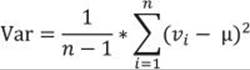
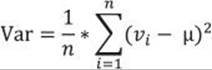
This is the formula for the variance of a sample, used as an estimator for the variance of the population. Now imagine that your data represents the complete population, and the mean value is unknown. Then all the observations contribute to the variance calculation equally, and the degrees of freedom make no sense. The variance of a population is defined, then, with the same formula as the MSD:
Transact-SQL includes an aggregate function that calculates the variance for a sample as an estimator for the variance of the population (the VARP function) and a function that calculates the variance for the population (the VAR function). A query that uses them is very simple. The following query calculates both variances and also compares them in two ways: by dividing them, and by dividing the number of cases minus one with the number of cases, to show that the difference is only a result of the degrees of freedom used in calculating the variance of a sample as an estimator for the variance of the population:
SELECT VAR(salesamount) AS populationvariance,
VARP(salesamount) AS samplevariance,
VARP(salesamount) / VAR(salesamount) AS samplevspopulation1,
(1.0 * COUNT(*) - 1) / COUNT(*) AS samplevspopulation2
FROM dbo.SalesAnalysis;
The query returns the following result:
populationvariance samplevariance samplevspopulation1 samplevspopulation2
------------------ ------------------ ------------------- -------------------
1074263.80010215 1073765.30181904 0.99953596287703 0.999535962877
If your sample is big enough, the difference is negligible. In the example I am using when analyzing the sales, the data represents the complete sales—that is, the population. Therefore, using the variance for the population is more appropriate for a correct analysis here.
Standard deviation and the coefficient of the variation
To compensate for having the deviations squared, you can take the square root of the variance. This is the definition of the standard deviation (σ):
![]()
Of course, you can use the same formula to calculate the standard deviation of the population, and the standard deviation of a sample as an estimator of the standard deviation for the population; just use the appropriate variance in the formula.
I derived the absolute measures of the spread, the interpretation of which is quite evident for a single variable—the bigger the values of the measures are, the more spread out the variable in the observations is. But the absolute measures cannot be used to compare the spread between two or more variables. Therefore, I need to derive relative measures. I can derive the relative measures of the spread for any of the absolute measures mentioned, but I will limit myself to only the most popular one: the standard deviation. The definition of the relative standard deviation or the Coefficient of the Variation (CV) is a simple division of the standard deviation with the mean value:
![]()
T-SQL includes two aggregate functions to calculate the standard deviation for the population (STDEVP) and to calculate the standard deviation for a sample (STDEV) as an estimator for the standard deviation for the population. Calculating standard deviation and the coefficient of the variation, therefore, is simple and straightforward. The following query calculates both standard deviations for the salesamount column and the coefficient of the variation for the salesamount and discountamount columns:
SELECT STDEV(salesamount) AS populationstdev,
STDEVP(salesamount) AS samplestdev,
STDEV(salesamount) / AVG(salesamount) AS CVsalesamount,
STDEV(discountamount) / AVG(discountamount) AS CVdiscountamount
FROM dbo.SalesAnalysis;
The query returns the following result:
populationstdev samplestdev CVsalesamount CVdiscountamount
------------------ ------------------ ----------------- ------------------
1036.46697974521 1036.2264722632 1.64906211150028 3.25668651182147
You can see that the discountamount variable varies more than the salesamount variable.
Higher population moments
By comparing the mean and the median, you can determine whether your distribution is skewed. Can you also measure this skewness? Of course, the answer is yes. However, before defining and calculating this measure, you need to define the normal and standard-normal distributions.
Normal and standard normal distributions
Normal distributions are a family of distributions that have the same general shape. Normal distributions are symmetric, with scores more concentrated in the middle than in the tails. Normal distributions are described as bell shaped. The bell curve is also called a Gaussian curve, in honor of Karl Friedrich Gauss.
The height of a normal distribution is specified mathematically with two parameters: the mean (μ) and the standard deviation (σ). Constants in the formula are π (3.14159) and e (the base of natural logarithms = 2.718282). The formula for the normal distribution is
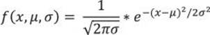
The normal distribution is a commonly occurring, continuous probability distribution. It is a function that tells the probability that any real observation will fall between any two real limits or real numbers, as the curve approaches zero on either side. Normal distributions are extremely important in statistics and are often used in the natural and social sciences for real-valued random variables whose distributions are not known. Simply said, if you do not know the distribution of a continuous variable in advance, you assume that it follows the normal distribution.
The standard normal distribution (Z distribution) is a normal distribution with a mean of 0 and a standard deviation of 1. You can easily calculate the z values of the standard normal distribution by normalizing the x values of the normal distribution:
![]()
Figure 8-1 shows the standard normal distribution curve.
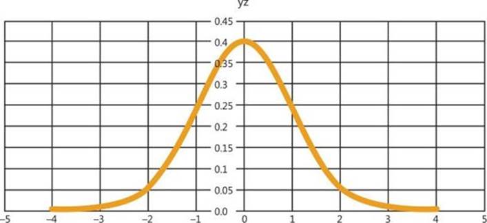
FIGURE 8-1 Standard normal distribution.
You can see that the probability that a value lies more than couple of standard deviations away from the mean gets low very quickly. The figure shows the probability function calculated only to four standard deviations from the mean on both sides. Later in this chapter, I will show you how to calculate this probability.
Skewness
Skewness is a parameter that describes asymmetry in a random variable’s probability distribution. Skewness characterizes the degree of asymmetry of a distribution around its mean. Positive skewness indicates a distribution with an asymmetric tail extending toward more positive values. Negative skewness indicates a distribution with an asymmetric tail extending toward more negative values.
Skewness tells you that values in the tail on one side of the mean (depending on whether the skewness is positive or negative) might still be valid and you don’t want to deal with them as outliers. Outliers are rare and far out-of-bounds values that might be erroneous. Therefore, knowing the skewness of a variable does not give you only information about the variable distribution; it also can help you when you cleanse your data.
The formula for the skewness is
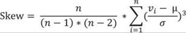
Similar to the mean-absolute-deviation and the mean-squared-deviation formulas, the formula for the skewness uses the mean value. In addition, there is also the standard deviation in the formula. I calculated the MAD and MSD with inefficient code; I calculated the mean in advance, and then the MAD and MSD. This means I scanned all the data twice. I did not bother to optimize the code for the MAD and MSD, because I used these two measures of a spread only to lead you slowly to the variance and the standard deviation, which are commonly used. For the variance and the standard deviation, aggregate functions are included in T-SQL. There is no skewness aggregate function; therefore, you need to optimize the code. I want to calculate the skewness by scanning the data only once.
I use a bit of mathematics for this optimization. First, I expand the formula for the subtraction of the mean from the ith value cubed.
(vi – μ)3 = vi3 – 3vi2μ + 3viμ2 – μ3
Then I use the fact that the sum is distributive over the product, as shown in the formula for two values only:
3v1μ2 + 3v2μ2 = 3μ2(v1 + v2)
This formula can be generalized for all values:
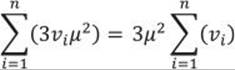
Of course, I can do the same mathematics for the remaining elements of the expanded formula for the subtraction and calculate all the aggregates I need with a single pass through the data in a common table expression (CTE), and then calculate the skewness with these aggregates, like the following query shows:
WITH SkewCTE AS
(
SELECT SUM(salesamount) AS rx,
SUM(POWER(salesamount,2)) AS rx2,
SUM(POWER(salesamount,3)) AS rx3,
COUNT(salesamount) AS rn,
STDEV(salesamount) AS stdv,
AVG(salesamount) AS av
FROM dbo.SalesAnalysis
)
SELECT
(rx3 - 3*rx2*av + 3*rx*av*av - rn*av*av*av)
/ (stdv*stdv*stdv) * rn / (rn-1) / (rn-2) AS skewness
FROM SkewCTE;
The query returns the following result:
skewness
----------------------
6.78219500069942
Positive skewness means that the distribution of the salesamount variable has a longer tail on the right side, extending more toward the positive values.
Kurtosis
Kurtosis characterizes the relative peakedness or flatness of a distribution compared with the normal distribution. A positive kurtosis means a higher peak around the mean and some extreme values on any side tail. A negative kurtosis indicates a relatively flat distribution. For a peaked distribution, consider that values far from the mean in any direction might be correct. The formula for the kurtosis is
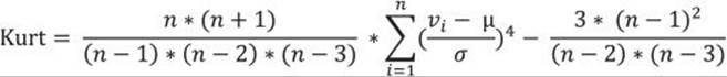
As with the skewness, you can see that the formula for the kurtosis also includes the mean and the standard deviation. To get an efficient query, I start with expanding the subtraction again:
(vi – μ)4 = vi4 – 4vi3μ + 6vi2μ2 – 4viμ3 + μ4
After that, I can use the fact that the sum is distributive over the product again, and calculate the kurtosis with a single scan of the data, as the following query shows:
WITH KurtCTE AS
(
SELECT SUM(salesamount) AS rx,
SUM(POWER(salesamount,2)) AS rx2,
SUM(POWER(salesamount,3)) AS rx3,
SUM(POWER(salesamount,4)) AS rx4,
COUNT(salesamount) AS rn,
STDEV(salesamount) AS stdv,
AVG(salesamount) AS av
FROM dbo.SalesAnalysis
)
SELECT
(rx4 - 4*rx3*av + 6*rx2*av*av - 4*rx*av*av*av + rn*av*av*av*av)
/ (stdv*stdv*stdv*stdv) * rn * (rn+1) / (rn-1) / (rn-2) / (rn-3)
- 3.0 * (rn-1) * (rn-1) / (rn-2) / (rn-3) AS kurtosis
FROM KurtCTE;
The result for the kurtosis of the salesamount variable is
kurtosis
----------------------
68.7756494703992
The value for the kurtosis tells you that there are many values of the salesamount variable around the mean, because there is a high peak in the distribution around the mean; however, the variable has quite a few values far away from the mean in either or both of the tails as well.
Mean, standard deviation, skewness, and kurtosis are also called the four population moments. Mean uses the values on the first degree in the calculation; therefore, it is the first population moment. Standard deviation uses the squared values and is therefore the second population moment. Skewness is the third, and kurtosis is the fourth population moment. All together, they give you a very good estimation of the population distribution.
Skewness and kurtosis with CLR UDAs
The queries for calculating skewness and kurtosis are more complex than the queries earlier in the chapter. Now imagine you need to calculate these two values in groups. Calculating mean and standard deviation in groups is simple, because you have appropriate T-SQL aggregate functions, which can be used together with the GROUP BY clause. However, calculating skewness and kurtosis in groups with T-SQL expressions only leads to more complex queries.
Calculating skewness and kurtosis in groups would be simple if there were appropriate T-SQL aggregate functions. You can actually expand the list of the T-SQL aggregate functions with user-defined aggregate functions. However, you can’t define a user-defined aggregate (UDA) in T-SQL. You need a Common Language Runtime (CLR) language for this—for example, Visual C#. You can use either a SQL Server Database Project template or a simple Class Library template in Microsoft Visual Studio with the appropriate programming languages installed. Refer to books online for details on how to create such a project. Then you can simply copy the following C# code for the skewness and kurtosis UDAs, which uses the same mathematics as the T-SQL solutions for an efficient calculation with a single scan of the data:
using System;
using System.Data;
using System.Data.SqlClient;
using System.Data.SqlTypes;
using Microsoft.SqlServer.Server;
[Serializable]
[SqlUserDefinedAggregate(
Format.Native,
IsInvariantToDuplicates = false,
IsInvariantToNulls = true,
IsInvariantToOrder = true,
IsNullIfEmpty = false)]
public struct Skew
{
private double rx; // running sum of current values (x)
private double rx2; // running sum of squared current values (x^2)
private double r2x; // running sum of doubled current values (2x)
private double rx3; // running sum of current values raised to power 3 (x^3)
private double r3x2; // running sum of tripled squared current values (3x^2)
private double r3x; // running sum of tripled current values (3x)
private Int64 rn; // running count of rows
public void Init()
{
rx = 0;
rx2 = 0;
r2x = 0;
rx3 = 0;
r3x2 = 0;
r3x = 0;
rn = 0;
}
public void Accumulate(SqlDouble inpVal)
{
if (inpVal.IsNull)
{
return;
}
rx = rx + inpVal.Value;
rx2 = rx2 + Math.Pow(inpVal.Value, 2);
r2x = r2x + 2 * inpVal.Value;
rx3 = rx3 + Math.Pow(inpVal.Value, 3);
r3x2 = r3x2 + 3 * Math.Pow(inpVal.Value, 2);
r3x = r3x + 3 * inpVal.Value;
rn = rn + 1;
}
public void Merge(Skew Group)
{
this.rx = this.rx + Group.rx;
this.rx2 = this.rx2 + Group.rx2;
this.r2x = this.r2x + Group.r2x;
this.rx3 = this.rx3 + Group.rx3;
this.r3x2 = this.r3x2 + Group.r3x2;
this.r3x = this.r3x + Group.r3x;
this.rn = this.rn + Group.rn;
}
public SqlDouble Terminate()
{
double myAvg = (rx / rn);
double myStDev = Math.Pow((rx2 - r2x * myAvg + rn * Math.Pow(myAvg, 2))
/ (rn - 1), 1d / 2d);
double mySkew = (rx3 - r3x2 * myAvg + r3x * Math.Pow(myAvg, 2) -
rn * Math.Pow(myAvg, 3)) /
Math.Pow(myStDev,3) * rn / (rn - 1) / (rn - 2);
return (SqlDouble)mySkew;
}
}
[Serializable]
[SqlUserDefinedAggregate(
Format.Native,
IsInvariantToDuplicates = false,
IsInvariantToNulls = true,
IsInvariantToOrder = true,
IsNullIfEmpty = false)]
public struct Kurt
{
private double rx; // running sum of current values (x)
private double rx2; // running sum of squared current values (x^2)
private double r2x; // running sum of doubled current values (2x)
private double rx4; // running sum of current values raised to power 4 (x^4)
private double r4x3; // running sum of quadrupled current values raised to power 3 (4x^3)
private double r6x2; // running sum of squared current values multiplied by 6 (6x^2)
private double r4x; // running sum of quadrupled current values (4x)
private Int64 rn; // running count of rows
public void Init()
{
rx = 0;
rx2 = 0;
r2x = 0;
rx4 = 0;
r4x3 = 0;
r4x = 0;
rn = 0;
}
public void Accumulate(SqlDouble inpVal)
{
if (inpVal.IsNull)
{
return;
}
rx = rx + inpVal.Value;
rx2 = rx2 + Math.Pow(inpVal.Value, 2);
r2x = r2x + 2 * inpVal.Value;
rx4 = rx4 + Math.Pow(inpVal.Value, 4);
r4x3 = r4x3 + 4 * Math.Pow(inpVal.Value, 3);
r6x2 = r6x2 + 6 * Math.Pow(inpVal.Value, 2);
r4x = r4x + 4 * inpVal.Value;
rn = rn + 1;
}
public void Merge(Kurt Group)
{
this.rx = this.rx + Group.rx;
this.rx2 = this.rx2 + Group.rx2;
this.r2x = this.r2x + Group.r2x;
this.rx4 = this.rx4 + Group.rx4;
this.r4x3 = this.r4x3 + Group.r4x3;
this.r6x2 = this.r6x2 + Group.r6x2;
this.r4x = this.r4x + Group.r4x;
this.rn = this.rn + Group.rn;
}
public SqlDouble Terminate()
{
double myAvg = (rx / rn);
double myStDev = Math.Pow((rx2 - r2x * myAvg + rn * Math.Pow(myAvg, 2))
/ (rn - 1), 1d / 2d);
double myKurt = (rx4 - r4x3 * myAvg + r6x2 * Math.Pow(myAvg, 2)
- r4x * Math.Pow(myAvg, 3) + rn * Math.Pow(myAvg, 4)) /
Math.Pow(myStDev, 4) * rn * (rn + 1)
/ (rn - 1) / (rn - 2) / (rn - 3) -
3 * Math.Pow((rn - 1), 2) / (rn - 2) / (rn - 3);
return (SqlDouble)myKurt;
}
}
Then you can build the project and later deploy the assembly (the .dll file) to your SQL Server instance. Of course, you can also use the project with the source code or the pre-built assembly provided with the accompanying code for the book.
Once your assembly is built, you need to deploy it. The first step is to enable the CLR in your SQL Server instance:
EXEC sp_configure 'clr enabled', 1;
RECONFIGURE WITH OVERRIDE;
Then you deploy the assembly. Deploying an assembly means importing it into a database. SQL Server does not rely on .dll files on disk. You can deploy an assembly from Visual Studio directly, or you can use the T-SQL CREATE ASSEMBLY command. The following command assumes that the DescriptiveStatistics.dll file exists in the C:\temp folder.
CREATE ASSEMBLY DescriptiveStatistics
FROM 'C:\temp\DescriptiveStatistics.dll'
WITH PERMISSION_SET = SAFE;
After you import the assembly to your database, you can create the user-defined aggregates with the CREATE AGGREGATE command. The following two commands create the skewness and the kurtosis UDAs:
-- Skewness UDA
CREATE AGGREGATE dbo.Skew(@s float)
RETURNS float
EXTERNAL NAME DescriptiveStatistics.Skew;
GO
-- Kurtosis UDA
CREATE AGGREGATE dbo.Kurt(@s float)
RETURNS float
EXTERNAL NAME DescriptiveStatistics.Kurt;
GO
After you deploy the UDAs, you can use them in the same way as you do standard T-SQL aggregate functions. For example, the following query calculates the skewness and the kurtosis for the salesamount variable:
SELECT dbo.Skew(salesamount) AS skewness,
dbo.Kurt(salesamount) AS kurtosis
FROM dbo.SalesAnalysis;
The result of the query is
skewness kurtosis
---------------------- ----------------------
6.78219499972001 68.7756494631014
Of course, now when you have the UDAs, you can use them to calculate the skewness and the kurtosis in groups as well. The following query calculates the four population moments for the salesamount continuous variable in groups of the employeecountry discrete variable:
SELECT employeecountry,
AVG(salesamount) AS mean,
STDEV(salesamount) AS standarddeviation,
dbo.Skew(salesamount) AS skewness,
dbo.Kurt(salesamount) AS kurtosis
FROM dbo.SalesAnalysis
GROUP BY employeecountry;
The result is
employeecountry mean standarddeviation skewness kurtosis
--------------- ------------- ---------------------- ------------------ ------------------
UK 665.538450 1151.18458127003 5.25006816518545 34.9789294559445
USA 615.269533 992.247411594278 7.56357332529894 88.6908404800727
You can see from the higher values for the skewness and the kurtosis that the salesamount variable has a more important right tail for the USA employees. You can probably conclude that there are some big customers from the USA that placed quite bigger orders than the average customers.
Linear dependencies
I dealt with analyses of a single variable so far in this chapter. Now it is time to check whether two selected variables are independent or somehow related. In statistics, you start with the null hypothesis. The null hypothesis is a general statement or default position that there is no relationship between two measured variables. Then you try to prove or reject the hypothesis with statistical analyses. I am going to analyze linear relationships only.
As you already know, there are discrete and continuous variables. I will explain and develop code for analyzing relationships between two continuous variables, between two discrete variables, and between one continuous variable and one discrete variable.
Analyzing relationships between pairs of variables many times is the goal of doing an analysis. In addition, analyzing these relationships is useful as a first step to prepare for some deeper analysis—for example, an analysis that uses data-mining methods. Relationships found between pairs of variables help you select variables for more complex methods. For example, imagine you have one target variable and you want to explain its states with a couple of input variables. If you find a strong relationship between a pair of input variables, you can omit one and consider only the other one in your further, more complex analytical process. Thus, you reduce the complexity of the problem.
Two continuous variables
I will start by measuring the strength of the relationship of two continuous variables. I will define three measures: the covariance, the correlation coefficient, and the coefficient of determination. Finally, I will express one variable as a function of the other, using the linear regression formula.
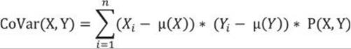
Covariance
Imagine you are dealing with two variables with a distribution of values as shown (for the sake of brevity, in a single table) in Table 8-2.
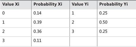
TABLE 8-2 Distribution of two variables
The first variable can have four different states, and the second variable can have three. Of course, these two variables actually represent two continuous variables with many more possible states; however, for the sake of providing a simpler explanation, I limited the number of possible states.
If the variables are truly independent, you can expect the same distribution of Y over every value of X and vice versa. You can easily compute the probability of each possible combination of the values of both variables: the probability of each combination of values of two independent variables is simply a product of the separate probabilities of each value:
P(Xi, Yi) = P(Xi) * P(Yi)
According to the formula, you can calculate an example as follows:
P(X=1, Y=2): P(1,2) = P(X1) * P(Y2) = 0.39 * 0.50 = 0.195
This is the expected probability for independent variables. But you have a different situation now, as shown in Table 8-3. There you see a cross-tabulation of X and Y with distributions of X and Y shown on the margins (the rightmost column and the bottommost row) and measured distributions of combined probabilities in the middle cells.
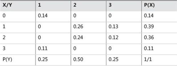
TABLE 8-3 Combined and marginal probabilities
I want to measure the deviation of the actual from the expected probabilities in the intersection cells. Remember the formula for the variance of one variable? Let’s write the formula once again, this time for both variables, X and Y:
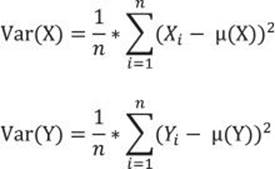
I will start measuring the covariance of a variable with itself. Let’s take an example of variable Z, which has only three states (1, 2, and 3), and for each state it has one value only. You can imagine a SQL Server table with three rows, one column Z, and a different value in each row. The probability of each value is 0.33, or exactly 1 / (number of rows)—that is, 1 divided by 3. Table 8-4 shows this variable cross-tabulated with itself. To distinguish between vertical and horizontal representations of the same variable Z, let’s call the variable “Z vertical” and “Z horizontal.”
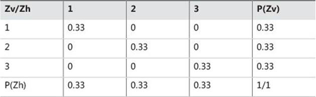
TABLE 8-4 A variable cross-tabulated with itself
The formula for the variance of a single variable can be expanded to a formula that measures how the variable covaries with itself:
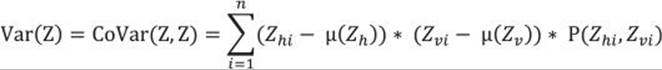
This formula seems suitable for two variables as well. Of course, it was my intention to develop a formula to measure the spread of combined probabilities of two variables. I simply replace one variable—for example, the “horizontal” Z with X, and the other one (the “vertical” Z) with Y—and get the formula for the covariance:
Now I can calculate the covariance for two continuous variables from my sales analysis view. I can replace the probability for the combination of the variables P(X, Y) with probability for each of the n rows combined with itself—that is, with 1 / n2—and the sum of these probabilities forn rows with 1 / n, because each row has an equal probability. Here is the query that calculates the covariance of the variables salesamount and discountamount:
WITH CoVarCTE AS
(
SELECT salesamount as val1,
AVG(salesamount) OVER () AS mean1,
discountamount AS val2,
AVG(discountamount) OVER() AS mean2
FROM dbo.SalesAnalysis
)
SELECT
SUM((val1-mean1)*(val2-mean2)) / COUNT(*) AS covar
FROM CoVarCTE;
The result of this query is
covar
------------------
76375.801912
Covariance indicates how two variables, X and Y, are related to each other. When large values of both variables occur together, the deviations are both positive (because Xi – Mean(X) > 0 and Yi – Mean(Y) > 0), and their product is therefore positive. Similarly, when small values occur together, the product is positive as well. When one deviation is negative and one is positive, the product is negative. This can happen when a small value of X occurs with a large value of Y and the other way around. If positive products are absolutely larger than negative products, the covariance is positive; otherwise, it is negative. If negative and positive products cancel each other out, the covariance is zero. And when do they cancel each other out? Well, you can imagine such a situation quickly—when two variables are really independent. So the covariance evidently summarizes the relation between variables:
![]() If the covariance is positive, when the values of one variable are large, the values of the other one tend to be large as well.
If the covariance is positive, when the values of one variable are large, the values of the other one tend to be large as well.
![]() If the covariance is negative, when the values of one variable are large, the values of the other one tend to be small.
If the covariance is negative, when the values of one variable are large, the values of the other one tend to be small.
![]() If the covariance is zero, the variables are independent.
If the covariance is zero, the variables are independent.
Correlation and coefficient of determination
When I derived formulas for the spread of the distribution of a single variable, I wanted to have the possibility of comparing the spread of two or more variables. I had to derive a relative measurement formula—the coefficient of the variation (CV):
![]()
Now I want to compare the two covariances computed for two pairs of the variables. Let’s again try to find a similar formula—let’s divide the covariance with something. It turns out that a perfect denominator is a product of the standard deviations of both variables. This is the formula for the correlation coefficient:
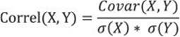
The reason that the correlation coefficient is a useful measure of the relation between two variables is that it is always bounded: –1 <= Correl <= 1. Of course, if the variables are independent, the correlation is zero, because the covariance is zero. The correlation can take the value 1 if the variables have a perfect positive linear relation (if you correlate a variable with itself, for example). Similarly, the correlation would be –1 for the perfect negative linear relation. The larger the absolute value of the coefficient is, the more the variables are related. But the significance depends on the size of the sample. A coefficient over 0.50 is generally considered to be significant. However, there could be a casual link between variables as well. To correct the too-large value of the correlation coefficient, it is often squared and thus diminished. The squared coefficient is called the coefficient of determination (CD):
CD(X, Y) = Correl(X, Y)2
In statistics, when the coefficient of determination is above 0.20, you typically can reject the null hypothesis, meaning you can say that the two continuous variables are not independent and that, instead, they are correlated. The following query calculates the covariance, the correlation coefficient, and the coefficient of determination for the salesamount and discountamount variables:
WITH CoVarCTE AS
(
SELECT salesamount as val1,
AVG(salesamount) OVER () AS mean1,
discountamount AS val2,
AVG(discountamount) OVER() AS mean2
FROM dbo.SalesAnalysis
)
SELECT
SUM((val1-mean1)*(val2-mean2)) / COUNT(*) AS covar,
(SUM((val1-mean1)*(val2-mean2)) / COUNT(*)) /
(STDEVP(val1) * STDEVP(val2)) AS correl,
SQUARE((SUM((val1-mean1)*(val2-mean2)) / COUNT(*)) /
(STDEVP(val1) * STDEVP(val2))) AS CD
FROM CoVarCTE;
The result is
covar correl CD
-------------- ---------------------- ----------------------
76375.801912 0.550195368441261 0.302714943454215
From the result, you can see that you can safely reject the null hypothesis for these two variables. The salesamount and discountamount variables are positively correlated: the higher the salesamount is, the higher the discountamount is. Of course, this is what you could expect.
Before concluding this part, let me point out the common misuse of the correlation coefficient. Correlation does not mean causation. This is a very frequent error. When people see high correlation, they incorrectly infer that one variable causes or influences the values of the other one. Again, this is not true. Correlation has no direction. In addition, remember that I measure linear dependencies only. Even if the correlation coefficient is zero, it still does not mean that the variables are independent (or not related at all). You can say that, if the two variables are independent, they are also uncorrelated, but if they are uncorrelated, they are not necessarily independent.
Linear regression
If the correlation coefficient is significant, you know there is some linear relation between the two variables. I would like to express this relation in a functional way—that is, one variable as a function of the other one. The linear function between two variables is a line determined by its slope and its intercept. Logically, the goal is to calculate the slope and the intercept. You can quickly imagine that the slope is somehow connected with the covariance.
But I start to develop the formula for the slope from another perspective. I start with the formula for the line, where the slope is denoted with b and the intercept with a:
Y’ = a + b * X
You can imagine that the two variables you are analyzing form a two-dimensional plane. Their values define coordinates of the points in the plane. You are searching for a line that fits all the points best. Actually, it means that you want the points to fall as close to the line as possible. You need the deviations from the line—that is, the difference between the actual value for Yi and the line value Y’. If you use simple deviations, some are going to be positive and others negative, so the sum of all deviations is going to be zero for the best-fit line. A simple sum of deviations, therefore, is not a good measure. You can square the deviations, like they are squared to calculate the mean squared deviation. To find the best-fit line, you have to find the minimal possible sum of squared deviations. I am not going to do the complete derivation of the formula here; after this brief explanation, I am just showing the final formulas for the slope and the intercept:
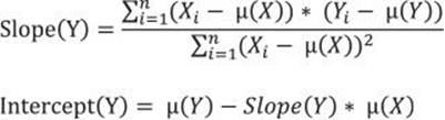
If you look back at the formulas for the covariance and the mean squared deviation, you can see that the numerator of the slope is really connected with the covariance, while the denominator closely resembles the mean squared deviation of the independent variable.
As I go along, I have nonchalantly started to use terms like “independent” and implicitly “dependent” variables. How do I know which one is the cause and which one is the effect? Well, in real life it is usually easy to qualify the roles of the variables. In statistics, just for the overview, I can calculate both combinations, Y as a function of X and X as a function of Y, as well. So I get two lines, which are called the first regression line and the second regression line.
After I have the formulas, it is easy to write the queries in T-SQL, as shown in the following query:
WITH CoVarCTE AS
(
SELECT salesamount as val1,
AVG(salesamount) OVER () AS mean1,
discountamount AS val2,
AVG(discountamount) OVER() AS mean2
FROM dbo.SalesAnalysis
)
SELECT Slope1=
SUM((val1 - mean1) * (val2 - mean2))
/SUM(SQUARE((val1 - mean1))),
Intercept1=
MIN(mean2) - MIN(mean1) *
(SUM((val1 - mean1)*(val2 - mean2))
/SUM(SQUARE((val1 - mean1)))),
Slope2=
SUM((val1 - mean1) * (val2 - mean2))
/SUM(SQUARE((val2 - mean2))),
Intercept2=
MIN(mean1) - MIN(mean2) *
(SUM((val1 - mean1)*(val2 - mean2))
/SUM(SQUARE((val2 - mean2))))
FROM CoVarCTE;
The result is
Slope1 Intercept1 Slope2 Intercept2
---------------------- ---------------------- ---------------------- ----------------------
0.0711289532105013 -3.56166730855091 4.25586107754898 453.41491444211
Contingency tables and chi-squared
Covariance and correlation measure dependencies between two continuous variables. During the calculation, they both use the means of the two variables involved. (Correlation also uses standard deviation.) Mean values and other population moments make no sense for categorical (nominal) variables.
If you denote “Clerical” as 1 and “Professional” as 2 for the variable occupation, what does the average of 1.5 mean? You have to find another test for dependencies—a test that does not rely on the numeric values. You can use contingency tables and the chi-squared test.
Contingency tables are used to examine the relationship between subjects’ scores on two qualitative or categorical variables. They show the actual and expected distribution of cases in a cross-tabulated (pivoted) format for the two variables. Table 8-5 is an example of the actual (or observed) and expected distribution of cases over the occupation column (on rows) and the maritalstatus column (or columns):
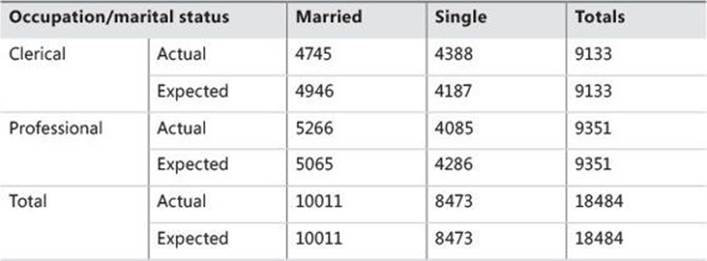
TABLE 8-5 A contingency table example
If the columns are not contingent on the rows, the row and column frequencies are independent. The test of whether the columns are contingent on the rows is called the chi-squared test of independence. The null hypothesis is that there is no relationship between row and column frequencies. Therefore, there should be no difference between the observed (O) and expected (E) frequencies.
Chi-squared is simply a sum of normalized squared frequencies’ deviations (that is, the sum of squares of differences between observed and expected frequencies divided by expected frequencies). This formula is also called the Pearson chi-squared formula.
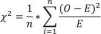
There are already prepared tables with critical points for the chi-squared distribution. If the calculated chi-squared value is greater than a critical value in the table for the defined degrees of freedom and for a specific confidence level, you can reject the null hypothesis with that confidence (which means the variables are interdependent). The degrees of freedom is the product of the degrees of freedom for columns (C) and rows (R):
DF = (C – 1) * (R – 1)
Table 8-6 is an example of a chi-squared critical-points table. Greater differences between expected and actual data produce a larger chi-squared value. The larger the chi-squared value is, the greater the probability is that there really is a significant difference. The Probability row in the table shows you the maximal probability that the null hypothesis holds when the chi-squared value is greater than or equal to the value in the table for the specific degrees of freedom.
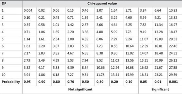
TABLE 8-6 Chi-squared critical points
For example, you have calculated chi-squared for two discrete variables. The value is 16, and the degrees of freedom are 7. Search for the first smaller and first bigger value for the chi-squared in the row for degrees of freedom 7 in Table 8-6. The values are 14.07 and 18.48. Check the appropriate probability for these two values, which are 0.05 and 0.01. This means there is less than a 5% probability that the two variables are independent, and more than a 1% probability that they are independent. This is a significant percentage, meaning you can say the variables are dependent with more than a 95% probability.
Calculating chi-squared is not that simple with T-SQL. It is not a problem to get the actual (observed) frequencies; the problem is getting the expected frequencies. For example, the following query uses the PIVOT operator to get the actual frequencies of combinations of states of thecategoryname and employeecountry variables from the sales analysis view:
SELECT categoryname, [USA],[UK]
FROM (SELECT categoryname, employeecountry, orderid FROM dbo.SalesAnalysis) AS S
PIVOT(COUNT(orderid) FOR employeecountry
IN([USA],[UK])) AS P
ORDER BY categoryname;
The query produces the following result:
categoryname USA UK
--------------- ----------- -----------
Beverages 294 110
Condiments 158 58
Confections 256 78
Dairy Products 240 126
Grains/Cereals 157 39
Meat/Poultry 131 42
Produce 96 40
Seafood 255 75
You can calculate expected frequencies from the marginal frequencies, or from the totals over rows and columns. The following query does this step by step, by calculating the observed frequencies for the combination of both variables’ states, and then observed frequencies for the first and second variables, and then observed total frequencies (total number of cases), and only after that the expected frequencies for the combination of both variables’ states, and finally it joins together the observed and expected frequencies:
WITH
ObservedCombination_CTE AS
(
SELECT categoryname, employeecountry, COUNT(*) AS observed
FROM dbo.SalesAnalysis
GROUP BY categoryname, employeecountry
),
ObservedFirst_CTE AS
(
SELECT categoryname, NULL AS employeecountry, COUNT(*) AS observed
FROM dbo.SalesAnalysis
GROUP BY categoryname
),
ObservedSecond_CTE AS
(
SELECT NULL AS categoryname, employeecountry, COUNT(*) AS observed
FROM dbo.SalesAnalysis
GROUP BY employeecountry
),
ObservedTotal_CTE AS
(
SELECT NULL AS categoryname, NULL AS employeecountry, COUNT(*) AS observed
FROM dbo.SalesAnalysis
),
ExpectedCombination_CTE AS
(
SELECT F.categoryname, S.employeecountry,
CAST(ROUND(1.0 * F.observed * S.observed / T.observed, 0) AS INT) AS expected
FROM ObservedFirst_CTE AS F
CROSS JOIN ObservedSecond_CTE AS S
CROSS JOIN ObservedTotal_CTE AS T
),
ObservedExpected_CTE AS
(
SELECT O.categoryname, O.employeecountry, O.observed, E.expected
FROM ObservedCombination_CTE AS O
INNER JOIN ExpectedCombination_CTE AS E
ON O.categoryname = E.categoryname
AND O.employeecountry = E.employeecountry
)
SELECT * FROM ObservedExpected_CTE;
It produces the following result:
categoryname employeecountry observed expected
--------------- --------------- ----------- -----------
Condiments UK 58 57
Produce UK 40 36
Dairy Products USA 240 270
Grains/Cereals UK 39 52
Seafood USA 255 243
Seafood UK 75 87
Confections USA 256 246
Meat/Poultry USA 131 127
Dairy Products UK 126 96
Beverages USA 294 298
Confections UK 78 88
Meat/Poultry UK 42 46
Beverages UK 110 106
Produce USA 96 100
Condiments USA 158 159
Grains/Cereals USA 157 144
Of course, the query is pretty inefficient. It scans the data many times. I am showing the query to help you more easily understand the process of calculating the expected frequencies. Alternatively, you can use window aggregate functions, which make this calculation much simpler. The following query uses only two common table expressions: the first one calculates just the observed frequencies for the combination of both variables’ states, and the second one uses the window aggregate functions to calculate the marginal and total frequencies and the expected frequencies for the combination of both variables’ states, while the outer query calculates the chi-squared and the degrees of freedom.
WITH ObservedCombination_CTE AS
(
SELECT categoryname AS onrows,
employeecountry AS oncols,
COUNT(*) AS observedcombination
FROM dbo.SalesAnalysis
GROUP BY categoryname, employeecountry
),
ExpectedCombination_CTE AS
(
SELECT onrows, oncols, observedcombination,
SUM(observedcombination) OVER (PARTITION BY onrows) AS observedonrows,
SUM(observedcombination) OVER (PARTITION BY oncols) AS observedoncols,
SUM(observedcombination) OVER () AS observedtotal,
CAST(ROUND(SUM(1.0 * observedcombination) OVER (PARTITION BY onrows)
* SUM(1.0 * observedcombination) OVER (PARTITION BY oncols)
/ SUM(1.0 * observedcombination) OVER (), 0) AS INT) AS expectedcombination
FROM ObservedCombination_CTE
)
SELECT SUM(SQUARE(observedcombination - expectedcombination)
/ expectedcombination) AS chisquared,
(COUNT(DISTINCT onrows) - 1) * (COUNT(DISTINCT oncols) - 1) AS degreesoffreedom
FROM ExpectedCombination_CTE;
Here is the result:
chisquared degreesoffreedom
---------------------- ----------------
22.2292997748233 7
Now you can read Table 8-6, which is the chi-squared critical-points table shown earlier. For 7 degrees of freedom, you can read the first lower and first higher values, which you can find in the last two columns: 18.48 and 24.32. Read the probability for the lower value—it is 0.01. You can say with more than a 99% probability that the categoryname and employeecountry variables are dependent. Apparently, employees from the USA sell more items in some product categories, while employees from the UK sell more items in other product categories.
Analysis of variance
Finally, it is time to check for linear dependencies between a continuous and a discrete variable. You can do this by measuring the variance between means of the continuous variable in different groups of the discrete variable. The null hypothesis here is that all variance between means is a result of the variance within each group. If you reject it, this means that there is some significant variance of the means between groups. This is also known as the residual, or unexplained, variance. You are analyzing the variance of the means, so this analysis is called the analysis of variance, or ANOVA.
You calculate the variance between groups MSA as the sum of squares of deviations of the group mean from the total mean times the number of cases in each group, with the degrees of freedom equal to the number of groups minus one. The formula is
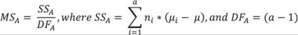
The discrete variable has discrete states, μ is the overall mean of the continuous variable, and μi is the mean in the continuous variable in the ith group of the discrete variable.
You calculate the variance within groups MSE as the sum over groups of the sum of squares of deviations of individual values from the group mean, with the degrees of freedom equal to the sum of the number of rows in each group minus one:
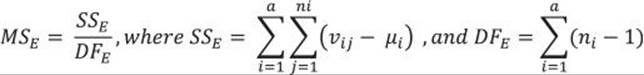
The individual value of the continuous variable is denoted as vij, μi is the mean in the continuous variable in the ith group of the discrete variable, and ni is the number of cases in the ith group of the discrete variable.
Once you have both variances, you calculate the so-called F ratio as the ratio between the variance between groups and the variance within groups:

A large F value means you can reject the null hypothesis. Tables for the cumulative distribution under the tails of F distributions for different degrees of freedom are already calculated. For a specific F value with degrees of freedom between groups and degrees of freedom within groups, you can get critical points where there is, for example, less than a 5% distribution under the F distribution curve up to the F point. This means that there is less than a 5% probability that the null hypothesis is correct (that is, there is an association between the means and the groups). If you get a large F value when splitting or sampling your data, the splitting or sampling was not random.
As I mentioned, you could now use the F value to search the F distribution tables. However, I want to show you how you can calculate the F probability on the fly. It is quite simple to calculate the cumulative F distribution using CLR code (for example, with a C# application). Unfortunately, the CLR FDistribution method, which performs the task, is implemented in a class that is not supported inside SQL Server. However, you can create a console application and then call it from SQL Server Management Studio using the SQLCMD mode. Here is the C# code for the console application that calculates the cumulative F distribution:
using System;
using System.Collections.Generic;
using System.Linq;
using System.Text;
using System.Windows.Forms.DataVisualization.Charting;
class FDistribution
{
static void Main(string[] args)
{
// Test input arguments
if (args.Length != 3)
{
Console.WriteLine("Please use three arguments: double FValue, int DF1, int DF2.");
//Console.ReadLine();
return;
}
// Try to convert the input arguments to numbers.
// FValue
double FValue;
bool test = double.TryParse(args[0], System.Globalization.NumberStyles.Float,
System.Globalization.CultureInfo.InvariantCulture.NumberFormat, out FValue);
if (test == false)
{
Console.WriteLine("First argument must be double (nnn.n).");
return;
}
// DF1
int DF1;
test = int.TryParse(args[1], out DF1);
if (test == false)
{
Console.WriteLine("Second argument must be int.");
return;
}
// DF2
int DF2;
test = int.TryParse(args[2], out DF2);
if (test == false)
{
Console.WriteLine("Third argument must be int.");
return;
}
// Calculate the cumulative F distribution function probability
Chart c = new Chart();
double result = c.DataManipulator.Statistics.FDistribution(FValue, DF1, DF2);
Console.WriteLine("Input parameters: " +
FValue.ToString(System.Globalization.CultureInfo.InvariantCulture.NumberFormat)
+ " " + DF1.ToString() + " " + DF2.ToString());
Console.WriteLine("Cumulative F distribution function probability: " +
result.ToString("P"));
}
}
The following query performs the one-way ANOVA, the analysis of variance using one input discrete variable, the categoryname variable, and the salesamount continuous variable:
WITH Anova_CTE AS
(
SELECT categoryname, salesamount,
COUNT(*) OVER (PARTITION BY categoryname) AS gr_casescount,
DENSE_RANK() OVER (ORDER BY categoryname) AS gr_denserank,
SQUARE(AVG(salesamount) OVER (PARTITION BY categoryname) -
AVG(salesamount) OVER ()) AS between_gr_SS,
SQUARE(salesamount -
AVG(salesamount) OVER (PARTITION BY categoryname))
AS within_gr_SS
FROM dbo.SalesAnalysis
)
SELECT N'Between groups' AS [Source of Variation],
SUM(between_gr_SS) AS SS,
(MAX(gr_denserank) - 1) AS df,
SUM(between_gr_SS) / (MAX(gr_denserank) - 1) AS MS,
(SUM(between_gr_SS) / (MAX(gr_denserank) - 1)) /
(SUM(within_gr_SS) / (COUNT(*) - MAX(gr_denserank))) AS F
FROM Anova_CTE
UNION
SELECT N'Within groups' AS [Source of Variation],
SUM(within_gr_SS) AS SS,
(COUNT(*) - MAX(gr_denserank)) AS df,
SUM(within_gr_SS) / (COUNT(*) - MAX(gr_denserank)) AS MS,
NULL AS F
FROM Anova_CTE;
The query uses a bit of creativity to calculate the degrees of freedom. It calculates the degrees of freedom between groups by calculating the dense rank of the groups and subtracting 1. Dense rank has the same value for all groups. By finding the maximal dense rank, you can find the number of groups. The query also calculates the degrees of freedom within groups as the total number of cases minus the number of groups. This way, everything can be calculated with a single scan of the data in the common table expression and in the outer query that refers to the common table expression. The outer query actually consists of two queries with unioned result sets. This is not necessary from the query perspective, and it might be even less efficient than a single query. However, I decided on the approach with the two unioned result sets to get the output that follows the standard statistical way of presenting the ANOVA results. Here is the output of the query:
Source of Variation SS df MS F
------------------- ------------------ ---------- ------------------ ----------------------
Between groups 55804413.9792925 7 7972059.13989894 7.57962783966074
Within groups 2258159811.46234 2147 1051774.48135181 NULL
The last thing to do is check the significance level of the F value for the specified degrees of freedom. I deployed the FDistribution.exe console application to the C:\temp folder. In SQL Server Management Studio, you can enable the SQLCMD mode in the Query menu. Then you can execute the following command:
!!C:\temp\FDistribution 7.57962783966074 7 2147
With these input parameters, which are the result of the analysis-of-variance query, you get the following result:
Input parameters: 7.57962783966074 7 2147
Cumulative F distribution function probability: 0.00 %
The result means that there is less than a 0.01% probability that the two variables would be independent. Of course, some product categories include cheaper products while others include more expensive products; thus, the difference in the mean of the sales amount is the result of the variability between groups.
Definite integration
When checking whether I could prove or reject the null hypothesis, I used statistical tables—for example, for chi-squared distribution with specific degrees of freedom. For the F distribution, I used a CLR application instead of a statistical table. In addition, I kind of arbitrarily selected the threshold where I defined that the relationship between two variables is significant. The threshold was at 95% (or at 5% from the different angle of view), meaning that I could reject the null hypothesis with a 95% probability. The question is where do these tables come from, or how does the CLR application calculate the values ad hoc, and why did I select a threshold at 95%.
The tables are calculated from a distribution function. For example, there is a set of distribution functions for the chi-squared values: one function for each degree of freedom. You can calculate the area under the function for all possible values, the total area, and the area for a specific interval of values, which can be closed or open for one side—this would be the tail area. If you know the distribution function, you can calculate the area under the function with a definite integration. Then you can compare the specific area with the total area to find out the percentage of cases in the specific area.
Of course, there is no definite integration function in T-SQL. However, there are many ways for performing numerical integration and for calculating the numerical value of a definite integral. The trapezoidal rule can be implemented in a simple and efficient way in T-SQL code. You define a trapezium for the curve f(x) and then calculate the surface of the trapezium, like Figure 8-2 shows.
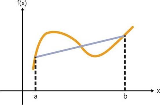
FIGURE 8-2 Trapezoidal rule for a definite integration.
The formula for the trapezoidal rule is
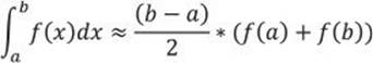
In the formula, a and b denote the values of the variable x, which defines the area for which the definite integral is approximately calculated.
By splitting the area under a curve into a bigger number of small trapeziums and then calculating and summing the area of these smaller trapeziums, you can get an accurate approximation for the numerical value of a definite integral.
By specifying n points in equal distance h, thus having a uniform grid for n–1 trapeziums, the formula becomes

From here, it is simple to implement definite integration in T-SQL. I will show it in an example where I will use the standard normal distribution, for which I already defined the distribution function. I am creating a temporary table that has two columns only—the z0 column, denoting theZ value, and yz, denoting the f(z0) value, the standard normal distribution function value. Then I populate the table with Z values between –4 and 4, with distance h equal to 0.01. The following code creates and populates the table:
-- Standard normal distribution table
CREATE TABLE #StdNormDist
(z0 DECIMAL(3,2) NOT NULL,
yz DECIMAL(10,9) NOT NULL);
GO
-- Insert the data
DECLARE @z0 DECIMAL(3,2), @yz DECIMAL(10,9);
SET @z0=-4.00;
WHILE @z0 <= 4.00
BEGIN
SET @yz=1.00/SQRT(2.00*PI())*EXP((-1.00/2.00)*SQUARE(@z0));
INSERT INTO #StdNormDist(z0,yz) VALUES(@z0, @yz);
SET @z0=@z0+0.01;
END
GO
Here are a few rows from the table:
z0 yz
--------------- --------------
-4.00 0.000133830
-3.99 0.000139285
-3.98 0.000144948
-3.97 0.000150825
...
-0.03 0.398762797
-0.02 0.398862500
-0.01 0.398922334
0.00 0.398942280
0.01 0.398922334
0.02 0.398862500
0.03 0.398762797
...
3.97 0.000150825
3.98 0.000144948
3.99 0.000139285
4.00 0.000133830
According to the trapezoidal rule for the definite integration, I have to take the first and last distribution function values of an interval for which I am calculating the area for only once, and all other distribution function values in the interval twice. I can also reverse the logic and calculate the double sum of all distribution function values, and then subtract the first and last values. I can get the first and last values in a range with the FIRST_VALUE and LAST_VALUE window analytic functions. For example, the following query calculates the percentage of the area below the standard normal distribution function between Z values of 0 (which is the mean value of the standard normal distribution) and 1 (which is the standard deviation of the standard normal distribution):
WITH ZvaluesCTE AS
(
SELECT z0, yz,
FIRST_VALUE(yz) OVER(ORDER BY z0 ROWS UNBOUNDED PRECEDING) AS fyz,
LAST_VALUE(yz)
OVER(ORDER BY z0
ROWS BETWEEN CURRENT ROW
AND UNBOUNDED FOLLOWING) AS lyz
FROM #StdNormDist
WHERE z0 >= 0 AND z0 <= 1
)
SELECT 100.0 * ((0.01 / 2.0) * (SUM(2 * yz) - MIN(fyz) - MAX(lyz))) AS pctdistribution
FROM ZvaluesCTE;
The result is
pctdistribution
---------------
34.134270
Now let me calculate the percentage of the area in the right tail from 1.96 standard deviations away from the mean. Because the standard normal distribution function is symmetric, I know that the area on the right side of the mean is exactly 50% of the total area. I use this fact in the following query:
WITH ZvaluesCTE AS
(
SELECT z0, yz,
FIRST_VALUE(yz) OVER(ORDER BY z0 ROWS UNBOUNDED PRECEDING) AS fyz,
LAST_VALUE(yz)
OVER(ORDER BY z0
ROWS BETWEEN CURRENT ROW
AND UNBOUNDED FOLLOWING) AS lyz
FROM #StdNormDist
WHERE z0 >= 0 AND z0 <= 1.96
)
SELECT 50 - 100.0 * ((0.01 / 2.0) * (SUM(2 * yz) - MIN(fyz) - MAX(lyz))) AS pctdistribution
FROM ZvaluesCTE;
The result is
pctdistribution
---------------
2.499885
This means that if you go approximately two standard deviations away from the mean in the standard normal distribution, the cumulative area under the distribution function under both left and right tails covers approximately 5% of the total area under the function. This number influenced the decision that the threshold for deciding whether the null hypothesis can be rejected or not is commonly set at 5%.
Moving averages and entropy
I have already shown in this chapter how to calculate the linear regression formula. You can use the linear regression for estimating unknown values for predictions. Even the mean itself is called an estimator; you can use it for simple estimations as well. However, both mean and linear regression include all values. When you deal with time-series data, you many times don’t want to do the prediction based on all past values, because older data might be completely irrelevant for current predictions. Or you might decide to put more stress on the recent values and less on the older values when estimating an unknown or new value. Moving averages can help you with this task.
I mentioned that you might want to check the linear dependencies of pairs of variables in the data overview stage, before doing some in-depth analysis. In addition, you also might want to check which variables can contribute to the analysis, which variables can give you some information, and which variables don’t give much information. I will show you how you can measure the amount of the information in a discrete variable.
Moving averages
In addition to being useful for estimation and prediction, moving averages are useful for data preparation as well. Moving averages smooth extreme values. Extreme values can influence a lot on all four population moments. If you smooth them, you can spot the trend in a much easier way than with the original values. Figure 8-3 shows a graph of the original values and two different moving averages, one that follows the original line better (WMA) and one that does more smoothing (SMA).
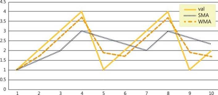
FIGURE 8-3 Moving-averages smoothing.
You probably already met moving averages in this book—they were mentioned, together with the query optimization techniques, in Chapter 4, “Grouping, pivoting, and windowing.” I am expanding the topic here to add different moving averages and to explain them more from the mathematical perspective than the query-optimization perspective.
The following code creates and populates a simple table I will use for explaining the moving averages:
CREATE TABLE dbo.MAvg
(id INT NOT NULL IDENTITY(1,1),
val FLOAT NULL);
GO
INSERT INTO dbo.MAvg(val) VALUES
(1), (2), (3), (4), (1), (2), (3), (4), (1), (2);
GO
This is the data from this demo table:
id val
----------- ------------
1 1
2 2
3 3
4 4
5 1
6 2
7 3
8 4
9 1
10 2
I also used this data for the graph in Figure 8-3.
Simple moving average
In financial applications, a simple moving average (SMA) is the unweighted mean of the previous n data. This is the moving average you learned about in Chapter 4. The formula for a simple moving average calculated over the last three values is
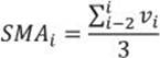
The following query calculates an SMA over last three values:
SELECT id, val,
ROUND
(AVG(val)
OVER (ORDER BY id
ROWS BETWEEN 2 PRECEDING
AND CURRENT ROW)
,2) AS SMA
FROM dbo.MAvg
ORDER BY id;
The query produces the following result:
id val SMA
----------- ---------- ----------------------
1 1 1
2 2 1.5
3 3 2
4 4 3
5 1 2.67
6 2 2.33
7 3 2
8 4 3
9 1 2.67
10 2 2.33
Weighted moving average
A weighted moving average (WMA) is any average that has multiplying factors to give different weights to data at different positions in the sample window. The sum of all weights must be equal to 1. With WMA, you can give more importance to the recent values and less importance to the older values. Here is the formula for a weighted moving average over the last two values:
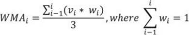
The following query calculates the WMA over the last two values, giving the weight 0.7 to the current value and weight 0.3 to the previous value:
DECLARE @A AS FLOAT;
SET @A = 0.7;
SELECT id, val,
LAG(val, 1, val) OVER (ORDER BY id) AS prevval,
@A * val + (1 - @A) *
(LAG(val, 1, val) OVER (ORDER BY id)) AS WMA
FROM dbo.MAvg
ORDER BY id;
The result of the query is
id val prevval WMA
----------- ---------- ---------- ----------
1 1 1 1
2 2 1 1.7
3 3 2 2.7
4 4 3 3.7
5 1 4 1.9
6 2 1 1.7
7 3 2 2.7
8 4 3 3.7
9 1 4 1.9
10 2 1 1.7
Exponential moving average
An exponential moving average (EMA) is a moving average that includes an unlimited list of previous values, meaning all previous values. It is also weighted, so again you typically put more importance on the more recent values. EMA is frequently used in economics for forecasting. The formula for EMA is
EMAi = α * vi + (1 – α) * EMAi–1, where EMA1 = v1
The problem with calculating the EMA is that the calculation for the current EMA uses the previous EMA. With window functions, SQL Server doesn’t expose the running calculation. You can’t refer to it in a query like you can do with a cursor. The following query shows an example of an EMA calculation with a cursor, where the weight (parameter) α is equal to 0.7:
DECLARE @CurrentEMA AS FLOAT, @PreviousEMA AS FLOAT,
@Id AS INT, @Val AS FLOAT,
@A AS FLOAT;
DECLARE @Results AS TABLE(id INT, val FLOAT, EMA FLOAT);
SET @A = 0.7;
DECLARE EMACursor CURSOR FOR
SELECT id, val
FROM dbo.MAvg
ORDER BY id;
OPEN EMACursor;
FETCH NEXT FROM EMACursor
INTO @Id, @Val;
SET @CurrentEMA = @Val;
SET @PreviousEMA = @CurrentEMA;
WHILE @@FETCH_STATUS = 0
BEGIN
SET @CurrentEMA = ROUND(@A * @Val + (1-@A) * @PreviousEMA, 2);
INSERT INTO @Results (id, val, EMA)
VALUES(@Id, @Val, @CurrentEMA);
SET @PreviousEMA = @CurrentEMA;
FETCH NEXT FROM EMACursor
INTO @Id, @Val;
END;
CLOSE EMACursor;
DEALLOCATE EMACursor;
SELECT id, val, EMA
FROM @Results;
GO
The query produces the following result:
id val EMA
----------- ---------- -----------
1 1 1
2 2 1.7
3 3 2.61
4 4 3.58
5 1 1.77
6 2 1.93
7 3 2.68
8 4 3.6
9 1 1.78
10 2 1.93
Of course, you know that using cursors does not produce the most efficient T-SQL code. Can you avoid the cursor? One option is to use a recursive common table expression, like the following query:
DECLARE @A AS FLOAT;
SET @A = 0.7;
WITH RnCTE AS
(
SELECT id, val,
ROW_NUMBER() OVER(ORDER BY id) AS rn
FROM dbo.MAvg
),
EMACTE AS
(
SELECT id, rn, val, val AS EMA
FROM RnCTE
WHERE id = 1
UNION ALL
SELECT C.id, C.rn, C.val,
ROUND (@A * C.val + (1 - @A) * P.EMA, 2) AS EMA
FROM EMACTE AS P
INNER JOIN RnCTE AS C
ON C.rn = P.rn + 1
)
SELECT id, val, EMA
FROM EMACTE;
Of course, this query is still not efficient, although it looks more set-oriented. A recursive CTE means a loop. Mimicking a recursive CTE with a WHILE loop also does not help much in optimizing the EMA calculation. I tried to convert the EMA formula to an equivalent formula that would use values only, and not the previous EMA in the formula. I started with expanding the EMA formula by replacing the previous EMA with the formula. Here is the process for expanding the EMA formula for five values:
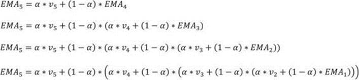
Because EMA1 is equal to the value 1, the formula uses the values only. After rearranging the equation, I found the generalized formula for calculating the EMA with values only:
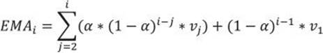
Now I am able to start searching for more efficient set-oriented solutions for calculating the EMA. I came up with the following query:
DECLARE @A AS FLOAT;
SET @A = 0.7;
WITH RnCTE AS
(
SELECT id, val,
ROW_NUMBER() OVER(ORDER BY id) AS rn,
FIRST_VALUE(val) OVER (ORDER BY id ROWS UNBOUNDED PRECEDING) AS v1
FROM dbo.MAvg
),
MaCTE AS
(
SELECT RN1.id AS id, Rn1.rn AS rn1, Rn2.rn AS rn2,
Rn1.v1, Rn1.val AS YI1, Rn2.val AS YI2,
MAX(RN2.rn) OVER (PARTITION BY RN1.rn) AS TRC
FROM RnCTE AS Rn1
INNER JOIN RnCTE AS Rn2
ON Rn1.rn >= Rn2.rn
)
SELECT id, MAX(YI1) AS val,
ROUND(
SUM(@A * POWER((1 - @A), (rn1 - rn2)) * YI2)
+
MAX(POWER((1 - @A), (TRC - 1)))
,2) AS EMA
FROM MaCTE
WHERE rn2 > 1
GROUP BY ID
UNION
SELECT 1, 1, 1
ORDER BY Id;
Unfortunately, although it is pretty complex, the query is still not efficient. It uses a non-equi join in the second common table expression, and this is a quadratic complexity. Therefore, with larger data sets, this query would quickly become much less efficient than the cursor. After many tries, I nearly gave up, and I started to think that the only reasonable way to calculate the EMA would be by using the cursor. I wrote a blog about this problem. After a couple of days, there was a comment on my blog. Quintin du Bruyn, a distinguished member of the SQL Server community, found the solution for an efficient set-oriented query for the EMA using the modified formula that uses the values only. Here is his query:
DECLARE @A AS FLOAT = 0.7, @B AS FLOAT;
SET @B = 1 - @A;
WITH cte_cnt AS
(
SELECT id, val,
ROW_NUMBER() OVER (ORDER BY id) - 1 as exponent
FROM dbo.MAvg
)
SELECT id, val,
ROUND(
SUM(CASE WHEN exponent=0 THEN 1
ELSE @A
END * val * POWER(@B, -exponent))
OVER (ORDER BY id) * POWER(@B, exponent)
, 2) AS EMA
FROM cte_cnt;
Therefore, you should never give up, and you should keep in mind that more people know more.
Entropy
Information theory is a branch of applied mathematics, electrical engineering, and computer science involving the quantification of information, developed by Claude E. Shannon. He wanted to find fundamental limits on signal-processing operations such as compressing data and on reliably storing and communicating data.
In a data set, you have a finite number of possible system states. If you have one binary variable, you have two possible states. Shannon defined information content in bits as a logarithm with a base two of the number of system states. For a discrete variable, the number of system states is the number of discrete values. Before performing some in-depth analysis, it is frequently useful to measure the amount of information in different variables. Variables with low information content—that is, with just very little info—might not be useful in the analysis. In information theory, information is the same thing as a surprise.
Introduction to entropy
Surprise measures the “unexpectedness” of a particular state. In a data set, surprise is quantified in terms of the probability (that is, relative frequency) of a particular state. If a system state has a lower probability, you are more surprised when it happens. So you get more information. Imagine that you buy five lottery tickets out of the 10 issued. How surprised are you if you win? How surprised are you if you buy only one ticket and win?
Information of a particular state i of the variable x is thus defined as a probability multiplied with the logarithm with base two of the probability:
I(x) = –P(xi) * LOG2(P(xi))
A negative sign is added because probability can take a value in an interval between 0 and 1, and a logarithm function returns negative values for this interval.
The total amount of information of a variable is a sum of all information of all its states. This total amount of information is called entropy. Therefore, the formula for the entropy of the variable x is:
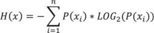
What is the maximal entropy for a specific variable? Suppose you have a variable with two states only. In one case, the distribution of the values between the two states is pretty unequal, one state probability is 0.9, and the other state probability is 0.1. In another case, both states have the same probability 0.5. The following query calculates the entropy for these two examples:
SELECT (-1) * (0.1*LOG(0.1,2) + 0.9*LOG(0.9,2)) AS unequaldistribution,
(-1) * (0.5*LOG(0.5,2) + 0.5*LOG(0.5,2)) AS equaldistribution;
The result is
unequaldistribution equaldistribution
---------------------- ----------------------
0.468995593589281 1
What you can see is that a more equal distribution means higher entropy. In a uniform distribution, where only one state is represented (that is, all values are equal to one constant value), the entropy is 0. Such a variable is useless for analysis. The entropy of a discrete variable is the highest when the values are distributed equally.
Let me test now the highest possible entropy for variables with a different number of possible states. The following query calculates the maximal possible entropy for variables with two, three, and four states, using the equal distribution of the values over the states:
SELECT (-1)*(2)*(1.0/2)*LOG(1.0/2,2) AS TwoStatesMax,
(-1)*(3)*(1.0/3)*LOG(1.0/3,2) AS ThreeStatesMax,
(-1)*(4)*(1.0/4)*LOG(1.0/4,2) AS FourStatesMax;
The result of the query is
TwoStatesMax ThreeStatesMax FourStatesMax
---------------------- ---------------------- ----------------------
1 1.58496235845298 2
From the mathematics, you can learn that
![]()
Therefore, the former query that calculates the maximal possible entropy for a different number of states can be simplified to
SELECT LOG(2,2) AS TwoStatesMax,
LOG(3,2) AS ThreeStatesMax,
LOG(4,2) AS FourStatesMax;
What you can see from the results is that with more states, the maximal possible entropy increases. For continuous variables, you can calculate the entropy by discretizing or binning them. Fewer bins means lower maximal possible entropy. Discretizing into bins with an equal number of cases means that you retain as much entropy as possible for the specified number of bins. This fact can also explain why SQL Server uses this equal area distribution for the statistics of the values of a column.
Calculating the entropy
It is quite simple to follow the entropy formula in T-SQL to calculate it. Besides calculating the entropy of a variable, you can also calculate the maximal possible entropy of the variable, and the percentage of the actual entropy from the maximal possible entropy for the variable. The following query does this calculation for the customercountry variable:
WITH ProbabilityCTE AS
(
SELECT customercountry,
COUNT(customercountry) AS StateFreq
FROM dbo.SalesAnalysis
WHERE customercountry IS NOT NULL
GROUP BY customercountry
),
StateEntropyCTE AS
(
SELECT customercountry,
1.0*StateFreq / SUM(StateFreq) OVER () AS StateProbability
FROM ProbabilityCTE
)
SELECT (-1)*SUM(StateProbability * LOG(StateProbability,2)) AS TotalEntropy,
LOG(COUNT(*),2) AS MaxPossibleEntropy,
100 * ((-1)*SUM(StateProbability * LOG(StateProbability,2))) /
(LOG(COUNT(*),2)) AS PctOfMaxPossibleEntropy
FROM StateEntropyCTE;
The result is
TotalEntropy MaxPossibleEntropy PctOfMaxPossibleEntropy
---------------------- ---------------------- -----------------------
3.91977859896801 4.39231742277876 89.2416968464042
Let me repeat the same query for the productcategory variable:
WITH ProbabilityCTE AS
(
SELECT categoryname,
COUNT(categoryname) AS StateFreq
FROM dbo.SalesAnalysis
WHERE categoryname IS NOT NULL
GROUP BY categoryname
),
StateEntropyCTE AS
(
SELECT categoryname,
1.0*StateFreq / SUM(StateFreq) OVER () AS StateProbability
FROM ProbabilityCTE
)
SELECT (-1)*SUM(StateProbability * LOG(StateProbability,2)) AS TotalEntropy,
LOG(COUNT(*),2) AS MaxPossibleEntropy,
100 * ((-1)*SUM(StateProbability * LOG(StateProbability,2))) /
(LOG(COUNT(*),2)) AS PctOfMaxPossibleEntropy
FROM StateEntropyCTE;
The result for the productcategory variable is
TotalEntropy MaxPossibleEntropy PctOfMaxPossibleEntropy
---------------------- ---------------------- -----------------------
2.90951317302341 3 96.9837724341137
You can see that the customercountry variable has a bigger maximal possible entropy, because it can occupy a value from a bigger amount of possible states, while the values of the productcategory variable are more equally distributed, and the actual entropy is closer to the maximal possible entropy.
Because this was the last query in this chapter, I have to clean my database:
DROP TABLE dbo.TestMedian;
DROP AGGREGATE dbo.Skew;
DROP AGGREGATE dbo.Kurt;
DROP ASSEMBLY DescriptiveStatistics;
EXEC sp_configure 'clr enabled', 0;
RECONFIGURE WITH OVERRIDE;
DROP TABLE #StdNormDist;
DROP TABLE dbo.MAvg;
Conclusion
In this chapter, you learned how to write many different queries that can help you when you have to develop a business intelligence application. You can extend your SQL Server toolset and your analytical queries a lot with the code from this chapter.
In addition, you also learned how to properly use the results of the queries and to understand the statistics behind them. Finally, I hope you also learned that optimizing a query does not always involve just finding the best possible execution plan. Analytical queries typically scan huge amounts of data, and optimizing with the classical nonclustered indexes does not bring any improvements. Of course, columnstore indexes can help with lowering disk IO. However, the real optimization technique you learned in this chapter is optimization with an algorithm. I showed many times how you can minimize the number of scans through the data by finding a different algorithm for some calculation and then rewriting the query to follow that algorithm.
For the queries in this chapter, I prepared a sales analysis view. In the introduction part, I also discussed the difference between discrete and continuous variables. Then I showed how to calculate the frequency distribution of a discrete variable efficiently and thus quickly get an overview of this distribution.
Then a big portion of this chapter dealt with continuous variables. I defined and showed how you can calculate the different measures of the descriptive statistics, from the measures for the center of distribution (including mode, median, and mean) through the measures for the spread of the distribution (including range, inter-quartile range, mean absolute deviation, mean squared deviation, variance, and standard deviation) to higher population moments (including skewness and kurtosis). I also explained and defined standard normal distribution and the statistical concept of degrees of freedom.
Another big portion of this chapter covered checking for linear dependencies. I developed queries that calculate the strength of the relationship for pairs of two continuous variables (including covariance, correlation coefficient, and coefficient of determination), two discrete variables (including contingency tables and a chi-squared test), and one discrete and one continuous variable with an analysis of variance. I also developed the calculations needed for the linear regression formula. On the fly, I also defined the statistical significance and showed how you can calculate the definite integration with T-SQL.
In the last part of this chapter, I covered a few unrelated topics useful for business-intelligence developers. From this material, you can learn about different moving averages, including simple, weighted, and exponential moving averages. You also can learn the basics of information theory and calculate the entropy of a variable to check whether, based on the information content, it can be used in further analysis.
Table 8-7 summarizes the statistical measures introduced in this chapter with a short definition.
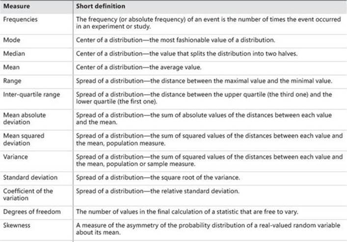
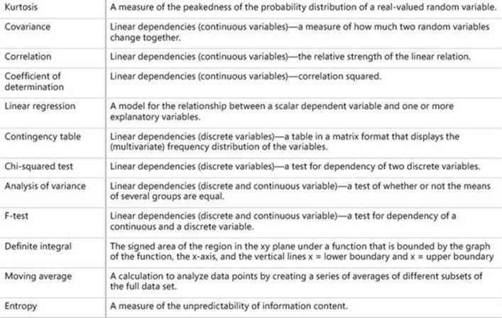
TABLE 8-7 Summary of the statistical measures introduced in this chapter