CCNP Routing and Switching ROUTE 300-101 Official Cert Guide (2015)
Part II. IGP Routing Protocols
Chapter 3. IPv6 Review and RIPng
This chapter covers the following subjects:
![]() Global Unicast Addressing, Routing, and Subnetting: This section introduces the concepts behind unicast IPv6 addresses, IPv6 routing, and how to subnet using IPv6, all in comparison to IPv4.
Global Unicast Addressing, Routing, and Subnetting: This section introduces the concepts behind unicast IPv6 addresses, IPv6 routing, and how to subnet using IPv6, all in comparison to IPv4.
![]() IPv6 Global Unicast Address Assignment: This section examines how global unicast addresses can be assigned to hosts and other devices.
IPv6 Global Unicast Address Assignment: This section examines how global unicast addresses can be assigned to hosts and other devices.
![]() Survey of IPv6 Addressing: This section examines all types of IPv6 addresses.
Survey of IPv6 Addressing: This section examines all types of IPv6 addresses.
![]() Configuring IPv6 Addresses on Cisco Routers: This section shows how to configure and verify static IPv6 addresses on Cisco routers.
Configuring IPv6 Addresses on Cisco Routers: This section shows how to configure and verify static IPv6 addresses on Cisco routers.
![]() RIP Next Generation (RIPng): This section compares and contrasts IPv4’s RIPv2 and IPv6’s RIPng routing protocols and shows how to configure RIPng.
RIP Next Generation (RIPng): This section compares and contrasts IPv4’s RIPv2 and IPv6’s RIPng routing protocols and shows how to configure RIPng.
In your CCNA studies, you were introduced to IP version 6 (IPv6) addressing, and you learned that IPv6 is the replacement protocol for IPv4. IPv6 provides the ultimate solution for the problem of running out of IPv4 addresses in the global Internet by using a 128-bit address, as opposed to IPv4’s 32-bit addresses. This gives IPv6 approximately 1038 total addresses, versus the mere (approximate) 4*109 total addresses in IPv4. However, many articles over the years have discussed when, if ever, a mass migration to IPv6 would take place. IPv6 has been the ultimate long-term solution for more than ten years, in part because the interim IPv4 solutions, including NAT/PAT, have thankfully delayed the day in which we truly run out of public unicast IP addresses.
With all the promise of IPv6 and its rapid adoption, most networking professionals are still most familiar with IPv4. Therefore, this chapter spends a few pages reviewing the fundamentals of IPv6 to set the stage for a discussion of IPv6 routing protocols.
IPv6 uses an updated version of the three popular interior gateway protocols (IGP) (RIP, EIGRP, and OSPF) to exchange routes inside an enterprise. Additionally, updates to the BGP version 4 standard, called multiprotocol extensions for BGP-4 (RFC 4760), allow the exchange of IPv6 routing information in the Internet.
This chapter demonstrates how to configure RIPng to support IPv6 routing. Upcoming chapters delve into IPv6 routing using EIGRP and OSPF version 3 (OSPFv3).
“Do I Know This Already?” Quiz
The “Do I Know This Already?” quiz allows you to assess whether you should read the entire chapter. If you miss no more than one of these ten self-assessment questions, you might want to move ahead to the “Exam Preparation Tasks” section. Table 3-1 lists the major headings in this chapter and the “Do I Know This Already?” quiz questions covering the material in those headings so that you can assess your knowledge of these specific areas. The answers to the “Do I Know This Already?” quiz appear in Appendix A.
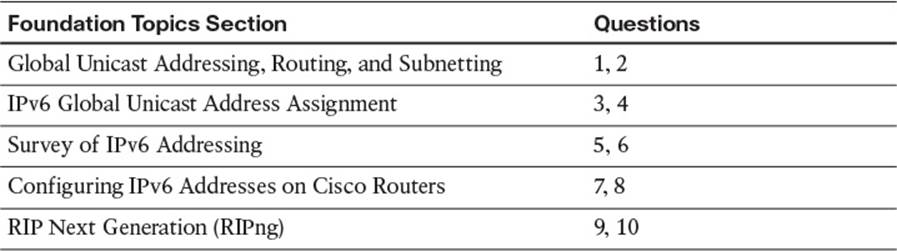
Table 3-1 “Do I Know This Already?” Foundation Topics Section-to-Question Mapping
1. Which of the following is the shortest valid abbreviation for FE80:0000:0000:0000:0010:0000:0000:0123?
a. FE80::10::123
b. FE8::1::123
c. FE80:0:0:0:10::123
d. FE80::10:0:0:123
2. An ISP has assigned prefix 3000:1234:5678::/48 to Company1. Which of the following terms would typically be used to describe this type of public IPv6 prefix?
a. Subnet prefix
b. ISP prefix
c. Global routing prefix
d. Registry prefix
3. Which of the following answers list either a protocol or function that can be used by a host to dynamically learn its own IPv6 address? (Choose two.)
a. Stateful DHCP
b. Stateless DHCP
c. Stateless autoconfiguration
d. Neighbor Discovery Protocol
4. Which of the following is helpful to allow an IPv6 host to learn the IP address of a default gateway on its subnet?
a. Stateful DHCP
b. Stateless RS
c. Stateless autoconfiguration
d. Neighbor Discovery Protocol
5. Which of the following answers lists a multicast IPv6 address?
a. 2000::1:1234:5678:9ABC
b. FD80::1:1234:5678:9ABC
c. FE80::1:1234:5678:9ABC
d. FF80::1:1234:5678:9ABC
6. Router R1 has two LAN interfaces and three serial interfaces enabled for IPv6. All the interfaces use link-local addresses automatically generated by the router. Which of the following could be the link-local address of R1’s interface S0/0?
a. FEA0::200:FF:FE11:0
b. FE80::200:FF:FE11:1111
c. FE80::0213:19FF:FE7B:0:1
d. FEB0::211:11FF:FE11:1111
7. Router R1 has the following configuration. Assuming that R1’s F0/0 interface has a MAC address of 0200.0011.1111, what IPv6 addresses will R1 list for interface F0/0 in the output of the show ipv6 interface brief command? (Choose two.)
interface f0/0
ipv6 address 2345:0:0:8::1/64
a. 2345:0:0:8::1
b. 2345:0:0:8:0:FF:FE11:1111
c. FE80::FF:FE11:1111
d. FE80:0:0:8::1
8. Router R1 lists the following output from a show command. Which of the following is true about R1?
R1# show ipv6 interface f0/0
FastEthernet0/0 is up, line protocol is up
IPv6 is enabled, link-local address is FE80::213:19FF:FE12:3456
No Virtual link-local address(es):
Global unicast address(es):
2000::4:213:19FF:FE12:3456, subnet is 2000:0:0:4::/64 [EUI]
Joined group address(es):
FF02::1
FF02::2
FF02::1:FF12:3456
a. R1’s solicited node multicast address is FF02::1:FF12:3456.
b. R1’s 2000::4:213:19FF:FE12:3456 address is a global unicast with all 128 bits statically configured.
c. Address FF02::2 is R1’s solicited node multicast.
d. R1’s solicited node multicast, not listed in this output, would be FF02::213:19FF:FE12:3456.
9. Which of the following features work the same in both RIPv2 and RIPng? (Choose three.)
a. Distance Vector Logic
b. Uses UDP
c. Uses RIP-specific authentication
d. Maximum useful metric of 15
e. Automatic route summarization
10. Router R1 currently has no configuration related to IPv6 or IPv4. The following configuration exists in a planning document, intended to be used to copy/paste into Router R1 to enable RIPng and IPv6 on interfaces Fa0/0 and S0/0/0. No other related configuration exists. Which of the following is true about RIPng on R1 after this configuration has been pasted into R1?
ipv6 unicast-routing
interface fa0/0
ipv6 rip one enable
ipv6 address 2000::1/64
interface s0/0/0
ipv6 address 2001::/64 eui-64
ipv6 rip one enable
a. RIPng will be enabled on no interfaces.
b. RIPng will be enabled on one interface.
c. RIPng will be enabled on two interfaces.
d. RIPng will advertise about prefixes connected to S0/0/0 and Fa0/0, but only send Updates on one interface.
Foundation Topics
The world has changed tremendously over the past 10–20 years as a result of the growth and maturation of the Internet and networking technologies in general. As recently as 1990, a majority of the general public did not know about nor use global networks to communicate, and when businesses needed to communicate, those communications mostly flowed over private networks. During the last few decades, the public Internet grew to the point where people in most parts of the world could connect to the Internet. Many companies connected to the Internet for a variety of applications, with the predominate applications being email and web access. During the first decade of the twenty-first century, the Internet has grown further to billions of addressable devices, with the majority of people on the planet having some form of Internet access. With that pervasive access came a wide range of applications and uses, including voice, video, collaboration, and social networking, with a generation that has grown up with this easily accessed global network.
The eventual migration to IPv6 will likely be driven by the need for more and more IP addresses. Practically every mobile phone supports Internet traffic, requiring the use of an IP address. Most new cars have the capability to acquire and use an IP address, along with wireless communications, allowing a car dealer to contact the customer when the car’s diagnostics detect a problem with the car. Some manufacturers have embraced the idea that all their appliances need to be IP-enabled.
Although the two biggest reasons why networks might migrate from IPv4 to IPv6 are the need for more addresses and mandates from government organizations, at least IPv6 includes some attractive features and migration tools. Some of those advantages are as follows:
![]() Address assignment features: IPv6 supports a couple of methods for dynamic address assignment, including DHCP and stateless autoconfiguration.
Address assignment features: IPv6 supports a couple of methods for dynamic address assignment, including DHCP and stateless autoconfiguration.
![]() Built-in support for address renumbering: IPv6 supports the ability to change the public IPv6 prefix used for all addresses in an enterprise, using the capability to advertise the current prefix with a short timeout and the new prefix with a longer lease life.
Built-in support for address renumbering: IPv6 supports the ability to change the public IPv6 prefix used for all addresses in an enterprise, using the capability to advertise the current prefix with a short timeout and the new prefix with a longer lease life.
![]() Built-in support for mobility: IPv6 supports mobility so that IPv6 hosts can move around an internetwork and retain their IPv6 addresses without losing current application sessions.
Built-in support for mobility: IPv6 supports mobility so that IPv6 hosts can move around an internetwork and retain their IPv6 addresses without losing current application sessions.
![]() Provider-independent and -dependent public address space: Internet Service Providers (ISP) can assign public IPv6 address ranges (dependent), or companies can register their own public address space (independent).
Provider-independent and -dependent public address space: Internet Service Providers (ISP) can assign public IPv6 address ranges (dependent), or companies can register their own public address space (independent).
![]() Aggregation: IPv6’s huge address space makes for much easier aggregation of blocks of addresses in the Internet, making routing in the Internet more efficient.
Aggregation: IPv6’s huge address space makes for much easier aggregation of blocks of addresses in the Internet, making routing in the Internet more efficient.
![]() No need for NAT/PAT: The huge public IPv6 address space removes the need for NAT/PAT, which avoids some NAT-induced application problems and makes for more efficient routing.
No need for NAT/PAT: The huge public IPv6 address space removes the need for NAT/PAT, which avoids some NAT-induced application problems and makes for more efficient routing.
![]() IPsec: Unlike IPv4, IPv6 requires that every IPv6 implementation support IPsec. IPv6 does not require that each device use IPsec, but any device that implements IPv6 must also have the ability to implement IPsec.
IPsec: Unlike IPv4, IPv6 requires that every IPv6 implementation support IPsec. IPv6 does not require that each device use IPsec, but any device that implements IPv6 must also have the ability to implement IPsec.
![]() Header improvements: Although it might seem like a small issue, the IPv6 header actually improves several things compared to IPv4. In particular, routers do not need to recalculate a header checksum for every packet, reducing per-packet overhead. Additionally, the header includes a flow label that allows easy identification of packets sent over the same single TCP or UDP connection.
Header improvements: Although it might seem like a small issue, the IPv6 header actually improves several things compared to IPv4. In particular, routers do not need to recalculate a header checksum for every packet, reducing per-packet overhead. Additionally, the header includes a flow label that allows easy identification of packets sent over the same single TCP or UDP connection.
![]() No broadcasts: IPv6 does not use Layer 3 broadcast addresses, instead relying on multicasts to reach multiple hosts with a single packet.
No broadcasts: IPv6 does not use Layer 3 broadcast addresses, instead relying on multicasts to reach multiple hosts with a single packet.
![]() Transition tools: As covered later in this chapter, IPv6 has many rich tools to help with the transition from IPv4 to IPv6.
Transition tools: As covered later in this chapter, IPv6 has many rich tools to help with the transition from IPv4 to IPv6.
This list includes many legitimate advantages of IPv6 over IPv4, but the core difference is IPv6 addressing. The first two sections of this chapter examine one particular type of IPv6 addresses, global unicast addresses, which have many similarities to IPv4 addresses (particularly public IPv4 addresses). The third section broadens the discussion to include all types of IPv6 addresses, and protocols related to IPv6 address assignment, default router discovery, and neighbor discovery. The fourth section looks at the router configuration commands for IPv6 addressing. The fifth section of this chapter examines RIP Next Generation (RIPng) and shows how it can be used to route traffic for IPv6 networks.
Global Unicast Addressing, Routing, and Subnetting
The original Internet design called for all organizations to register and be assigned one or more public IP networks (Class A, B, or C). By registering to use a particular public network address, the company or organization using that network was assured by the numbering authorities that no other company or organization in the world would be using the same addresses. As a result, all hosts in the world would have globally unique IP addresses.
From the perspective of the Internet infrastructure, in particular the goal of keeping Internet routers’ routing tables from getting too large, assigning an entire network to each organization helped to some degree. The Internet routers could ignore all subnets as defined inside an enterprise, instead having a route for each classful network. For example, if a company registered and was assigned Class B network 128.107.0.0/16, the Internet routers just needed one route for that entire network.
Over time, the Internet grew tremendously. It became clear by the early 1990s that something had to be done, or the growth of the Internet would grind to a halt when all the public IP networks were assigned and no more existed. Additionally, the IP routing tables in Internet routers were becoming too large for the router technology of that day. So, the Internet community worked together to come up with both some short-term and long-term solutions to two problems: the shortage of public addresses and the size of the routing tables.
The short-term solutions included a much smarter public address assignment policy in which public addresses were not assigned as only Class A, B, and C networks, but as smaller subdivisions (prefixes), reducing waste. Additionally, the growth of the Internet routing tables was reduced by smarter assignment of the actual address ranges based on geography. For example, assigning the Class C networks that begin with 198 to only a particular ISP in a particular part of the world allowed other ISPs to use one route for 198.0.0.0/8—in other words, all addresses that begin with 198—rather than a route for each of the 65,536 different Class C networks that begin with 198. Finally, Network Address Translation/Port Address Translation (NAT/PAT) achieved amazing results by allowing a typical home or small office to consume only one public IPv4 address, greatly reducing the need for public IPv4 addresses.
IPv6 provides the long-term solution to both problems (address exhaustion and Internet routing table size). The sheer size of IPv6 addresses takes care of the address exhaustion issue. The address assignment policies already used with IPv4 have been refined and applied to IPv6, with good results for keeping the size of IPv6 routing tables smaller in Internet routers. This section provides a general discussion of both issues, in particular how global unicast addresses, along with good administrative choices for how to assign IPv6 address prefixes, aid in routing in the global Internet. This section concludes with a discussion of subnetting in IPv6.
Global Route Aggregation for Efficient Routing
By the time the Internet community started serious work to find a solution to the growth problems in the Internet, many people already agreed that a more thoughtful public address assignment policy for the public IPv4 address space could help keep Internet routing tables much smaller and more manageable. IPv6 public address assignment follows these same well-earned lessons.
Note
The descriptions of IPv6 global address assignment in this section provide a general idea about the process. The process can vary from one Regional Internet Registry (RIR) to another and one Internet Service Provider (ISP) to another, based on many other factors.
The address assignment strategy for IPv6 is elegant, but simple, and can be roughly summarized as follows:
![]() Public IPv6 addresses are grouped (numerically) by major geographic region.
Public IPv6 addresses are grouped (numerically) by major geographic region.
![]() Inside each region, the address space is further subdivided by ISPs inside that region.
Inside each region, the address space is further subdivided by ISPs inside that region.
![]() Inside each ISP in a region, the address space is further subdivided for each customer.
Inside each ISP in a region, the address space is further subdivided for each customer.
The same organizations handle this address assignment for IPv6 as for IPv4. The Internet Corporation for Assigned Network Numbers (ICANN, www.icann.org) owns the process, with the Internet Assigned Numbers Authority (IANA) managing the process. IANA assigns one or more IPv6 address ranges to each RIR, of which there are five at the time of this publication, roughly covering North America, Central/South America, Europe, Asia/Pacific, and Africa. These RIRs then subdivide their assigned address space into smaller portions, assigning prefixes to different ISPs and other smaller registries, with the ISPs then assigning even smaller ranges of addresses to their customers.
The IPv6 global address assignment plan results in more efficient routing, as shown in Figure 3-1. The figure shows a fictitious company (Company1), which has been assigned an IPv6 prefix by a fictitious ISP, NA-ISP1 (indicating North American ISP number 1).

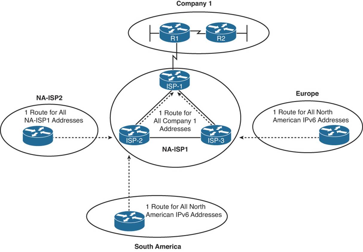
Figure 3-1 Conceptual View of IPv6 Global Routes
As shown in the figure, the routers installed by ISPs in other major geographies of the world can have a single route that matches all IPv6 addresses in North America. Although there might be hundreds of ISPs operating in North America, and hundreds of thousands of enterprise customers of those ISPs, and tens of millions of individual customers of those ISPs, all the public IPv6 addresses can be from one (or a few) very large address blocks—requiring only one (or a few) routes on the Internet routers in other parts of the world. Similarly, routers inside other ISPs in North America (for example, NA-ISP2, indicating North American ISP number 2 in the figure) can have one route that matches all address ranges assigned to NA-ISP1. Also, the routers inside NA-ISP1 just need to have one route that matches the entire address range assigned to Company1, rather than needing to know about all the subnets inside Company1.
Besides keeping the routers’ routing tables much smaller, this process also results in fewer changes to Internet routing tables. For example, if NA-ISP1 signed a service contract with another enterprise customer, NA-ISP1 could assign another prefix inside the range of addresses already assigned to NA-ISP1 by the American Registry for Internet Numbers (ARIN). The routers outside NA-ISP1’s network (that is, the majority of the Internet) do not need to know any new routes, because their existing routes already match the address range assigned to the new customer. The NA-ISP2 routers (another ISP) already have a route that matches the entire address range assigned to NA-ISP1, so they do not need any more routes. Likewise, the routers in ISPs in Europe and South America already have a route that works as well.
Conventions for Representing IPv6 Addresses
IPv6 conventions use 32 hexadecimal numbers, organized into 8 quartets of 4 hex digits separated by a colon, to represent a 128-bit IPv6 address, for example:
2340:1111:AAAA:0001:1234:5678:9ABC:1111
Each hex digit represents 4 bits, so if you want to examine the address in binary, the conversion is relatively easy if you memorize the values shown in Table 3-2.
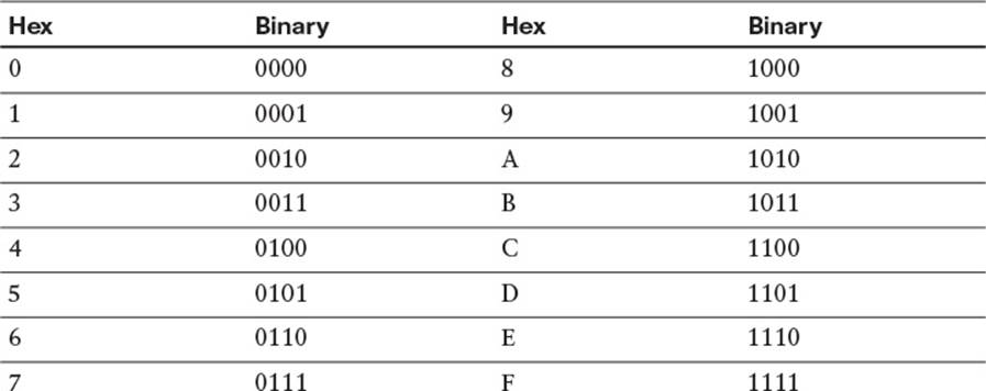
Table 3-2 Hexadecimal/Binary Conversion Chart
Writing or typing 32 hexadecimal digits, although more convenient than writing or typing 128 binary digits, can still be a pain. To make things a little easier, two conventions allow you to shorten what must be typed for an IPv6 address:
![]() Omit the leading 0s in any given quartet.
Omit the leading 0s in any given quartet.
![]() Represent one or more consecutive quartets of all hex 0s with “::” but only for one such occurrence in a given address.
Represent one or more consecutive quartets of all hex 0s with “::” but only for one such occurrence in a given address.
Note
For IPv6, a quartet is one set of four hex digits in an IPv6 address. There are eight quartets in each IPv6 address.
For example, consider the following address. The bold digits represent digits in which the address could be abbreviated.
FE00:0000:0000:0001:0000:0000:0000:0056
This address has two different locations in which one or more quartets have four hex 0s, so two main options exist for abbreviating this address—using the :: abbreviation in one or the other location. The following two options show the two briefest valid abbreviations:
FE00::1:0:0:0:56
FE00:0:0:1::56
In particular, note that the :: abbreviation, meaning “one or more quartets of all 0s,” cannot be used twice, because that would be ambiguous. So, the abbreviation FE00::1::56 would not be valid.
Conventions for Writing IPv6 Prefixes
IPv6 prefixes represent a range or block of consecutive IPv6 addresses. Just like routers use IPv4 subnets in IPv4 routing tables to represent ranges of consecutive addresses, routers use IPv6 prefixes to represent ranges of consecutive IPv6 addresses. The concepts mirror those of IPv4 addressing when using a classless view of the IPv4 address. Figure 3-2 reviews both the classful and classless views of IPv4 addresses, compared to the IPv6 view of addressing and prefixes.
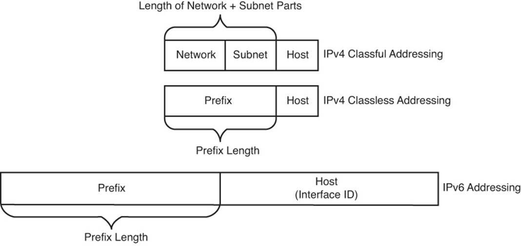
Figure 3-2 IPv4 Classless and Classful Addressing, IPv6 Addressing
First, for perspective, compare the classful and classless view of IPv4 addresses. Classful IPv4 addressing means that the class rules always identify part of the address as the network part. For example, the written value 128.107.3.0/24 (or 128.107.3.0 255.255.255.0) means 16 network bits (because the address is in a Class B network), 8 host bits (because the mask has 8 binary 0s), leaving 8 subnet bits. The same value, interpreted with classless rules, means prefix 128.107.3.0, prefix length 24. Classless addressing and classful addressing just give a slightly different meaning to the same numbers.
IPv6 uses a classless view of addressing, with no concept of classful addressing. Like IPv4, IPv6 prefixes list some prefix value, a slash, and then a numeric prefix length. Like IPv4 prefixes, the last part of the number, beyond the length of the prefix, will be represented by binary 0s. And finally, IPv6 prefix numbers can be abbreviated with the same rules as IPv6 addresses.
Note
IPv6 prefixes are often called IPv6 subnets. This book uses these terms interchangeably.
For example, consider the following IPv6 address that is assigned to a host on a LAN:
2000:1234:5678:9ABC:1234:5678:9ABC:1111/64
This value represents the full 128-bit IP address—there are no opportunities to even abbreviate this address. However, the /64 means that the prefix (subnet) in which this address resides is the subnet that includes all addresses that begin with the same first 64 bits as the address. Conceptually, it is the same logic as an IPv4 address. For example, address 128.107.3.1/24 is in the prefix (subnet) whose first 24 bits are the same values as address 128.107.3.1.
As with IPv4, when writing or typing a prefix, the bits past the end of the prefix length are all binary 0s. In the IPv6 address previously shown, the prefix in which the address resides would be
2000:1234:5678:9ABC:0000:0000:0000:0000/64
Which, when abbreviated, would be
2000:1234:5678:9ABC::/64
Next, consider one last fact about the rules for writing prefixes before seeing some examples. If the prefix length is not a multiple of 16, the boundary between the prefix and the interface ID (host) part of the address is inside a quartet. In such cases, the prefix value should list all the values in the last quartet in the prefix part of the value. For example, if the address just shown with a /64 prefix length instead had a /56 prefix length, the prefix would include all of the first three quartets (a total of 48 bits), plus the first 8 bits of the fourth quartet. The next 8 bits (last 2 hex digits) of the fourth octet should now be binary 0s, as part of the host portion of the address. So, by convention, the rest of the fourth octet should be written, after being set to binary 0s, as 9A00, which produces the following IPv6 prefix:
2000:1234:5678:9A00::/56
The following list summarizes some key points about how to write IPv6 prefixes.
![]() A prefix has the same value as the IP addresses in the group for the number of bits in the prefix length.
A prefix has the same value as the IP addresses in the group for the number of bits in the prefix length.
![]() Any bits after the prefix length number of bits are binary 0s.
Any bits after the prefix length number of bits are binary 0s.
![]() A prefix can be abbreviated with the same rules as IPv6 addresses.
A prefix can be abbreviated with the same rules as IPv6 addresses.
![]() If the prefix length is not on a quartet boundary, write down the value for the entire quartet.
If the prefix length is not on a quartet boundary, write down the value for the entire quartet.
Examples can certainly help in this case. Table 3-3 shows several sample prefixes, their format, and a brief explanation.
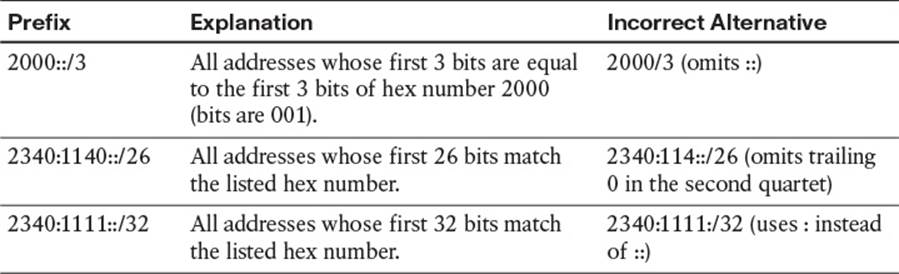
Table 3-3 Example IPv6 Prefixes and Their Meanings
Note which options are not allowed. For example, 2::/3 is not allowed instead of 2000::/3, because it omits the rest of the quartet, and a device could not tell whether 2::/3 means “hex 0002” or “hex 2000.”
Now that you understand a few of the conventions about how to represent IPv6 addresses and prefixes, a specific example can show how IANA’s IPv6 global unicast IP address assignment strategy can allow the easy and efficient routing previously shown in Figure 3-1.
Global Unicast Prefix Assignment Example
IPv6 standards reserve the range of addresses inside the 2000::/3 prefix as global unicast addresses. This address range includes all IPv6 addresses that begin with binary 001, or as more easily recognized, all IPv6 addresses that begin with a 2 or 3. IANA assigns global unicast IPv6 addresses as public and globally unique IPv6 addresses, as discussed using the example previously shown in Figure 3-1, allowing hosts using those addresses to communicate through the Internet without the need for NAT. In other words, these addresses fit the purest design for how to implement IPv6 for the global Internet.
Figure 3-3 shows an example set of prefixes that could result in a company (Company1) being assigned a prefix of 2340:1111:AAAA::/48.
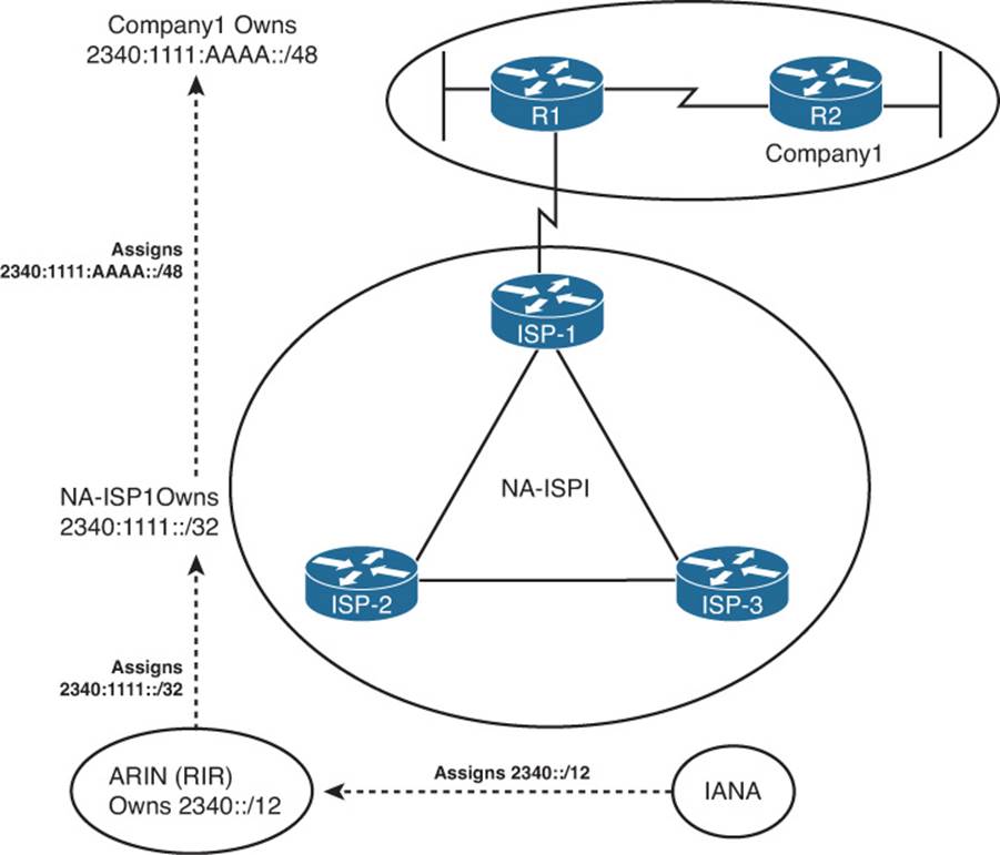
Figure 3-3 Example IPv6 Prefix Assignment in the Internet
The process starts with IANA, who owns the entire IPv6 address space and assigns the rights to a registry prefix to one of the RIRs (ARIN in this case, in North America). For the purposes of this chapter, assume that IANA assigns prefix 2340::/12 to ARIN. This assignment means that ARIN has the rights to assign any IPv6 addresses that begin with the first 12 bits of hex 2340 (binary value 0010 0011 0100). For perspective, that’s a large group of addresses: 2116 to be exact.
Next, NA-ISP1 asks ARIN for a prefix assignment. After ARIN ensures that NA-ISP1 meets some requirements, ARIN might assign ISP prefix 2340:1111::/32 to NA-ISP1. This too is a large group: 296 addresses to be exact. For perspective, this one address block might well be enough public IPv6 addresses for even the largest ISPs, without that ISP ever needing another IPv6 prefix.
Finally, Company1 asks its ISP, NA-ISP1, for the assignment of an IPv6 prefix. NA-ISP1 assigns Company1 the site prefix 2340:1111:AAAA::/48, which is again a large range of addresses: 280 in this case. A little later in this section, the text shows what Company1 could do with that prefix, but first, examine Figure 3-4, which presents the same concepts as in Figure 3-1, but now with the actual prefixes shown.
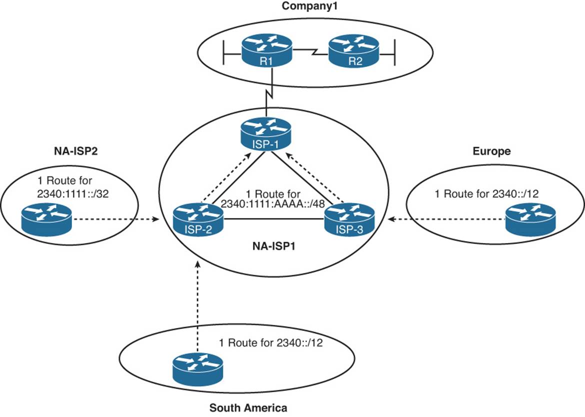
Figure 3-4 IPv6 Global Routing Concepts
The figure shows the perspectives of routers outside North America, routers from another ISP in North America, and other routers in the same ISP. Routers outside North America can use a route for prefix 2340::/12, knowing the IANA assigned this prefix to be used only by ARIN. This one route could match all IPv6 addresses assigned in North America. Routers in NA-ISP2, an example alternative ISP in North America, need one route for 2340:1111::/32, the prefix assigned to NA-ISP1. This one route could match all packets destined for all customers of NA-ISP1. Inside NA-ISP1, its routers need to know to which NA-ISP1 router to forward packets for that particular customer (named ISP-1 in this case), so the routes inside NA-ISP1’s routers list a prefix of 2340:1111:AAAA::/48.
Note
The /48 prefix assigned to a single company is called either a global routing prefix or a site prefix.
Subnetting Global Unicast IPv6 Addresses Inside an Enterprise
The original IPv4 Internet design called for each organization to be assigned a classful network number, with the enterprise subdividing the network into smaller address ranges by subnetting the classful network. This same concept of subnetting carries over from IPv4 to IPv6, with the enterprise subnetting its assigned global unicast prefix into smaller prefixes.
To better understand IPv6 subnetting, you can draw on either classful or classless IPv4 addressing concepts, whichever you find most comfortable. From a classless perspective, you can view the IPv6 addresses as follows:
![]() The prefix assigned to the enterprise by the ISP (the global routing prefix) acts like the prefix assigned for IPv4.
The prefix assigned to the enterprise by the ISP (the global routing prefix) acts like the prefix assigned for IPv4.
![]() The enterprise engineer extends the prefix length, borrowing host bits, to create a subnet part of the address with which to identify individual subnets.
The enterprise engineer extends the prefix length, borrowing host bits, to create a subnet part of the address with which to identify individual subnets.
![]() The remaining part of the addresses on the right, called either the interface ID or host part, works just like the IPv4 host part, uniquely identifying a host inside a subnet.
The remaining part of the addresses on the right, called either the interface ID or host part, works just like the IPv4 host part, uniquely identifying a host inside a subnet.
For example, Figure 3-5 shows a more detailed view of the Company1 enterprise network, shown in several of the previous figures in this chapter. The design concepts behind how many subnets are needed with IPv6 are identical to those of IPv4. Specifically, a subnet is needed for each VLAN and for each serial link, with the same Frame Relay subnetting options. In this case, two LANs and two serial links exist. So Company1 needs four subnets.
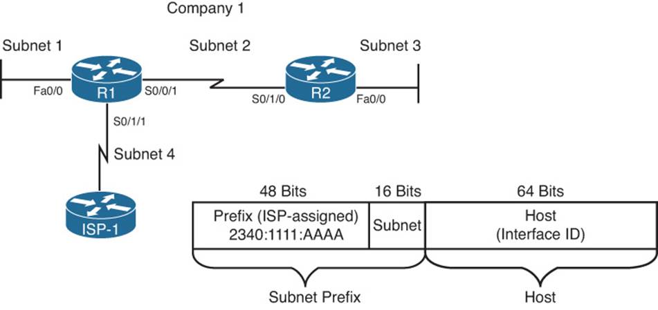
Figure 3-5 Company1—Needs Four Subnets
The figure also shows how the enterprise engineer extended the length of the prefix as assigned by the ISP (/48) to /64, thereby creating a 16-bit subnet part of the address structure. To create this extra 16-bit subnet field, the engineer uses the same concept as with IPv4 when choosing a subnet mask, by borrowing bits from the host field of an IPv4 address. In this case, think of the original host field (before subnetting) as having 80 bits, because the site prefix is 48 bits long, leaving 80 bits. The design in Figure 3-5 borrows 16 bits for the subnet field, leaving a measly 64 bits for the host field.
A bit of math about the design choices can help provide some perspective on the scale of IPv6. The 16-bit subnet field allows for 216, or 65,536, subnets—overkill for all but the very largest organizations or companies. (There are no worries about a zero or broadcast subnet in IPv6!) The host field is seemingly even more overkill: 264 hosts per subnet, which is more than 1,000,000,000,000,000,000 addresses per subnet. However, there is a good reason for this large host or interface ID part of the address. It allows one of the automatic IPv6 address assignment features to work well, as covered later in the “IPv6 Global Unicast Addresses Assignment” section of this chapter.
Figure 3-6 takes the concept to the conclusion, assigning the specific four subnets to be used inside Company1. Note that the figure shows the subnet fields and prefix lengths (64 in this case) in bold.
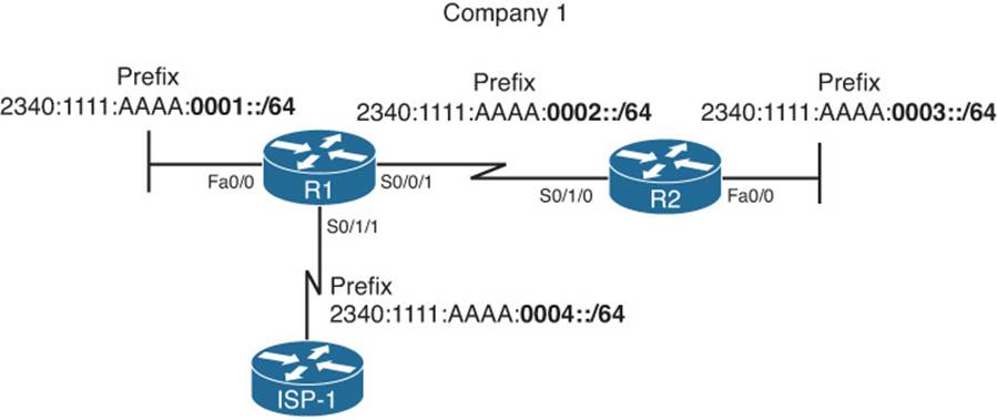
Figure 3-6 Company1—Four Subnets Assigned
Note
The subnet numbers in Figure 3-6 could be abbreviated slightly, removing the three leading 0s from the last shown quartets. The figure includes the leading 0s to show the entire subnet part of the prefixes.
Figure 3-6 just shows one option for subnetting the prefix assigned to Company1. However, any number of subnet bits could be chosen if the host field retained enough bits to number all hosts in a subnet. For example, a /112 prefix length could be used, extending the /48 prefix by 64 bits (four hex quartets). Then, for the design in Figure 3-6, you could choose the following four subnets:
2340:1111:AAAA::0001:0000/112
2340:1111:AAAA::0002:0000/112
2340:1111:AAAA::0003:0000/112
2340:1111:AAAA::0004:0000/112
By using global unicast IPv6 addresses, Internet routing can be very efficient. Enterprises can have plenty of IP addresses and plenty of subnets with no requirement for NAT functions to conserve the address space.
Prefix Terminology
Before wrapping up this section, you need to review a few terms. The process of global unicast IPv6 address assignment examines many different prefixes with many different prefix lengths. The text scatters a couple of more specific terms, but for easier study, Table 3-4 summarizes the four key terms with some reminders of what each means.
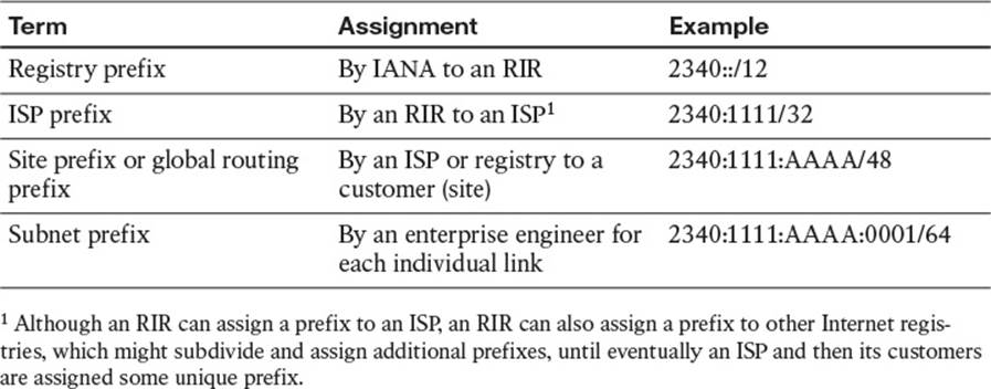
Table 3-4 Example IPv6 Prefixes and Their Meanings
IPv6 Global Unicast Addresses Assignment
This section still focuses on global unicast IPv6 addresses but now examines the topic of how a host, router interface, or other device knows what global unicast IPv6 address to use. Also, hosts (and sometimes routers) need to know a few other facts that can be learned at the same time as they learn their IPv6 address. So, this section also discusses how hosts can get all the following relevant information that lets them use their global unicast addresses:
![]() IP address
IP address
![]() IP subnet mask (prefix length)
IP subnet mask (prefix length)
![]() Default router IP address
Default router IP address
![]() DNS IP address(es)
DNS IP address(es)
IPv6 actually has four major options for IPv6 global unicast address assignment. This section looks at these options in the same order as listed in Table 3-5. Each method can use dynamic processes or static configuration, and each method can differ in terms of how a host or router gathers the other pertinent information (such as DNS IP addresses). Table 3-5 summarizes these main methods for easier review.
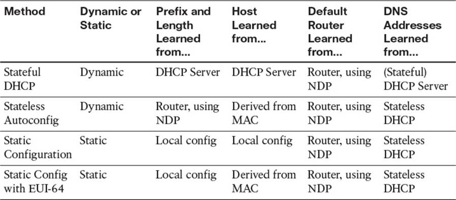
Table 3-5 Summary of IPv6 Address Assignment for Global Unicast Addresses
The rest of this section develops more detail about the topics in the table. Some of the processes work much like IPv4, and some do not. Regardless, as you work through the material, keep in mind one key fact about how IPv6 protocols approach the address assignment process:
IPv6 address assignment processes can split the IPv6 address assignment into two parts: the prefix/length assignment and the host (interface ID) assignment.
Stateful DHCP for IPv6
IPv6 hosts can use stateful DHCP to learn and lease an IP address and corresponding prefix length (mask) and the DNS IP address(es). The concept works basically like DHCP for IPv4. The host sends a (multicast) packet searching for the DHCP server. When a server replies, the DHCP client sends a message asking for a lease of an IP address, and the server replies, listing an IPv6 address, prefix length, and DNS IP addresses. (Note that Stateful DHCPv6 does not supply the default router information, instead relying on Neighbor Discovery Protocol [NDP] between the client and local routers.) The names and formats of the actual DHCP messages have changed quite a bit from IPv4 to IPv6. So, DHCPv4 and DHCPv6 actually differ in detail, but the basic process remains the same. (The term DHCPv4 refers to the version of DHCP used for IPv4, and the term DHCPv6 refers to the version of DHCP used for IPv6.)
DHCPv4 servers retain state information about each client, such as the IP address leased to that client and the length of time for which the lease is valid. In other words, DHCPv4 tracks the current state of DHCP clients. DHCPv6 servers happen to have two operational modes: stateful, in which the server does track state information, and stateless, in which the server does not track any state information. Stateful DHCPv6 servers fill the same role as the older DHCPv4 servers, whereas stateless DHCPv6 servers fill a different purpose as one part of the stateless autoconfiguration process. (Stateless DHCP, and its purpose, is covered in the upcoming section “Finding the DNS IP Addresses Using Stateless DHCP.”)
One difference between DHCPv4 and stateful DHCPv6 is that IPv4 hosts send IP broadcasts to find DHCP servers, whereas IPv6 hosts send IPv6 multicasts. IPv6 multicast addresses have a prefix of FF00::/8, meaning that the first 8 bits of an address are binary 11111111, or FF in hex. The multicast address FF02::1:2 (longhand FF02:0000:0000:0000:0000:0000:0001:0002) has been reserved in IPv6 to be used by hosts to send packets to an unknown DHCP server, with the routers working to forward these packets to the appropriate DHCP server.
Stateless Autoconfiguration
The second of the two options for dynamic IPv6 address assignment uses a built-in IPv6 feature called stateless autoconfiguration as the core tool. Stateless autoconfiguration allows a host to automatically learn the key pieces of addressing information—prefix, host, and prefix length—plus the default router IP address and DNS IP addresses. To learn or derive all these pieces of information, stateless autoconfiguration actually uses the following functions:
Step 1. IPv6 Neighbor Discovery Protocol (NDP), particularly the router solicitation and router advertisement messages, to learn the prefix, prefix length, and default router
Step 2. Some math to derive the interface ID (host ID) portion of the IPv6 address, using a format called EUI-64
Step 3. Stateless DHCP to learn the DNS IPv6 addresses
This section examines all three topics in order.
Learning the Prefix/Length and Default Router with NDP Router Advertisements
The IPv6 Neighbor Discovery Protocol (NDP) has many functions. One function allows IPv6 hosts to multicast a message that asks all routers on the link to announce two key pieces of information: the IPv6 addresses of routers willing to act as a default gateway and all known IPv6 prefixes on the link. This process uses ICMPv6 messages called a Router Solicitation (RS) and a Router Advertisement (RA).
For this process to work, before a host sends an RS message on a LAN, some router connected to that same LAN must already be configured for IPv6. The router must have an IPv6 address configured, and it must be configured to route IPv6 traffic. At that point, the router knows it can be useful as a default gateway, and it knows at least one prefix that can be useful to any clients on the LAN.
For example, Figure 3-7 shows a subset of the internetwork seen in Figures 3-5 and 3-6, with the same IPv6 addresses and subnets used. Router R1’s Fa0/0 has already been configured with an IPv6 address (2340:1111:AAAA:1:213:19FF:FE7B:5004/64) and has been configured to route IPv6 with the ipv6 unicast-routing global command.
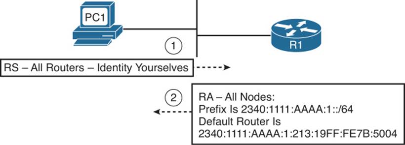
Figure 3-7 Example NDP RS/RA Process to Find the Default Routers
In the figure, host PC1, using stateless autoconfig, sends the RS message as an IPv6 multicast message destined to all IPv6 routers on the local link. The RS asks all routers to respond to the questions “What IPv6 prefix(s) is used on this subnet?” and “What is the IPv6 address(s) of any default routers on this subnet?” The figure also shows R1’s response (RA), listing the prefix (2340:1111:AAAA:1::/64), and with R1’s own IPv6 address as a potential default router.
Note
IPv6 allows multiple prefixes and multiple default routers to be listed in the RA message; Figure 3-7 just shows one of each for simplicity’s sake. One router’s RA would also include IPv6 addresses and prefixes advertised by other routers on the link.
IPv6 does not use broadcasts. In fact, there is no such thing as a subnet broadcast address, a network-wide broadcast address, or an equivalent of the all-hosts 255.255.255.255 broadcast IPv4 address. Instead, IPv6 makes use of multicast addresses. By defining different multicast IPv6 addresses for different functions, an IPv6 host that has no need to participate in a particular function can simply ignore those particular multicasts, reducing the impact on the host.
For example, the RS message needs to be received and processed only by routers, so the RS message’s destination IP address is FF02::2, which IPv6 reserves for use only by IPv6 routers. IPv6 defines that routers send RA messages to a multicast address intended for use by all IPv6 hosts on the link (FF02::1); routers do not forward these messages to other links. As a result, not only does the host that sent the RS message learn the information, but all other hosts on the link also learn the details. Table 3-6 summarizes some of the key details about the RS/RA messages.
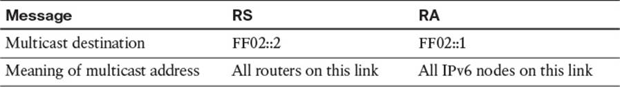
Table 3-6 Details of the RS/RA Process
Calculating the Interface ID Using EUI-64
Earlier in the chapter, Figure 3-5 showed the format of an IPv6 global unicast address with the second half of the address called the host ID or interface ID. The value of the interface ID portion of a global unicast address can be set to any value if no other host in the same subnet attempts to use the same value.
To automatically create a guaranteed-unique interface ID, IPv6 defines a method to calculate a 64-bit interface ID derived from that host’s MAC address. Because the burned-in MAC address should be literally globally unique, the derived interface ID should also be globally unique.
The EUI-64 process takes the 6-byte (48-bit) MAC address and expands it into a 64-bit value. To do so, IPv6 fills in 2 more bytes into the middle of the MAC address. IPv6 separates the original MAC address into two 3-byte halves and inserts hex FFFE in between the halves to form the Interface ID field of the IPv6 address. The conversion also requires flipping the seventh bit inside the IPv6 address, resulting in a 64-bit number that conforms to a convention called the EUI-64 format. The process is shown in Figure 3-8.
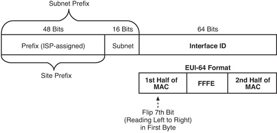
Figure 3-8 IPv6 Address Format with Interface ID and EUI-64
Although it might seem a bit convoluted, it works. Also, with a little practice, you can look at an IPv6 address and quickly notice the FFFE late in the address and then easily find the two halves of the corresponding interface’s MAC address.
For example, the following two lines list a host’s MAC address, and corresponding EUI-64 format Interface ID, assuming the use of an address configuration option that uses the EUI-64 format:
0034:5678:9ABC
0234:56FF:FE78:9ABC
Note
To change the seventh bit (left-to-right) in the example, we notice that hex 00 converts to binary 00000000. Then we change the seventh bit to 1 (00000010) and convert back to hex, which gives us hex 02 as the first two hexadecimal digits.
At this point in the stateless autoconfig process, a host knows its full IPv6 address and prefix length, plus a local router to use as the default gateway. The next section discusses how to complete the process using stateless DHCP.
Finding the DNS IP Addresses Using Stateless DHCP
Although the DHCP server function for IPv4 does not explicitly use the word “stateful” in its name, IPv4 DHCP servers keep state information about DHCP clients. The server keeps a record of the leased IP addresses and when the lease expires. The server typically releases the addresses to the same client before the lease expires, and if no response is heard from a DHCP client in time to renew the lease, the server releases that IP address back into the pool of usable IP addresses—again keeping that state information. The server also has configuration of the subnets in use and a pool of addresses in most subnets from which the server can assign IP addresses. It also serves other information, such as the default router IP addresses in each subnet, and the DNS servers’ IP addresses.
The IPv6 stateful DHCP server, as previously discussed in the section “Stateful DHCP for IPv6,” follows the same general idea. However, for IPv6, this server’s name includes the word stateful, to contrast it with the stateless DHCP server function in IPv6.
The stateless DHCP server function in IPv6 solves one particular problem: It supplies the DNS servers’ IPv6 addresses to clients. Because all hosts typically use the same small number of DNS servers, the stateless DHCP server does not need to keep track of any state information. An engineer simply configures the stateless DHCP server to know the IPv6 addresses of the DNS servers, and the server tells any host or other device that asks, keeping no record of the process.
Hosts that use stateless autoconfig also use stateless DHCP to learn the DNS servers’ IPv6 addresses.
Table 3-7 summarizes some of the key features of stateful and stateless DHCPv6.
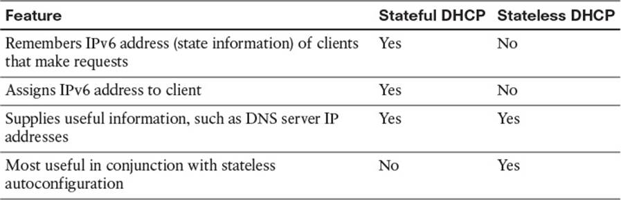
Table 3-7 Comparing Stateless and Stateful DHCPv6 Services
Static IPv6 Address Configuration
Two options exist for static configuration of IPv6 addresses:
![]() You configure the entire 128-bit IPv6 address.
You configure the entire 128-bit IPv6 address.
![]() You configure the 64-bit prefix and tell the device to use an EUI-64 calculation for the interface ID portion of the address.
You configure the 64-bit prefix and tell the device to use an EUI-64 calculation for the interface ID portion of the address.
Both options result in the host or router interface knowing its full 128-bit IPv6 address and prefix length.
When a host uses either form of static IPv6 address configuration, the host does not need to statically configure the other key pieces of information (default router and DNS IP addresses). The host can use the usual NDP process to discover any default routers and stateless DHCP to discover the DNS IPv6 addresses.
When a router uses static IPv6 address configuration, it might still use stateless DHCP to learn the DNS IP addresses. The upcoming section “Configuring IPv6 Addresses on Cisco Routers” shows several examples of this configuration.
Survey of IPv6 Addressing
So far, this chapter has focused on the IPv6 addresses that most closely match the concept of IPv4 addresses: the global unicast IPv6 addresses. This section now takes a broader look at IPv6 addressing, including some concepts that can be tied to older IPv4 concepts, and some that are unique to IPv6.
This section begins with a brief overview of IPv6 addressing. It then looks at unicast IPv6 addresses, along with a brief look at some of the commonly used multicast addresses. This section ends with a discussion of a couple of related protocols, namely, Neighbor Discovery Protocol (NDP) and Duplicate Address Detection (DAD).
Overview of IPv6 Addressing
The entire concept of global unicast addressing with IPv6 does have many similarities to IPv4. If viewing IPv4 addresses from a classless perspective, both IPv4 and IPv6 global unicast addresses have two parts: subnet plus host for IPv4 and prefix plus interface ID for IPv6. The format of the addresses commonly list a slash followed by the prefix length—a convention sometimes referred to as CIDR notation and other times as prefix notation. Subnetting works much the same, with a public prefix assigned by some numbering authority and the enterprise choosing subnet numbers, extending the length of the prefix to make room to number the subnets.
IPv6 addressing, however, includes several other types of unicast IPv6 addresses in addition to the global unicast address. Additionally, IPv6 defines other general categories of addresses, as summarized in the list that follows:
![]() Unicast: Like IPv4, hosts and routers assign these IP addresses to a single interface for the purpose of allowing that one host or interface to send and receive IP packets.
Unicast: Like IPv4, hosts and routers assign these IP addresses to a single interface for the purpose of allowing that one host or interface to send and receive IP packets.
![]() Multicast: Like IPv4, these addresses represent a dynamic group of hosts, allowing a host to send one packet that is then delivered to every host in the multicast group. IPv6 defines some special-purpose multicast addresses for overhead functions (such as NDP). IPv6 also defines ranges of multicast addresses for application use.
Multicast: Like IPv4, these addresses represent a dynamic group of hosts, allowing a host to send one packet that is then delivered to every host in the multicast group. IPv6 defines some special-purpose multicast addresses for overhead functions (such as NDP). IPv6 also defines ranges of multicast addresses for application use.
![]() Anycast: This address type allows the implementation of a nearest server among duplicate servers concept. This design choice allows servers that support the exact same function to use the exact same unicast IP address. The routers then forward a packet destined for such an address to the nearest server that is using the address.
Anycast: This address type allows the implementation of a nearest server among duplicate servers concept. This design choice allows servers that support the exact same function to use the exact same unicast IP address. The routers then forward a packet destined for such an address to the nearest server that is using the address.
Two big differences exist when comparing general address categories for IPv4 and IPv6:
![]() IPv6 adds the formal concept of Anycast IPv6 addresses as shown in the preceding list. IPv4 does not formally define an Anycast IP address concept, although a similar concept might be implemented in practice.
IPv6 adds the formal concept of Anycast IPv6 addresses as shown in the preceding list. IPv4 does not formally define an Anycast IP address concept, although a similar concept might be implemented in practice.
![]() IPv6 simply has no Layer 3 broadcast addresses. For example, all IPv6 routing protocols send Updates either to unicast or multicast IPv6 addresses, and overhead protocols such as NDP make use of multicasts as well. In IPv4, ARP still uses broadcasts, and the RIP version 1 routing protocol also uses broadcasts. With IPv6, there is no need to calculate a subnet broadcast address (hoorah!) and no need to make hosts process overhead broadcast packets meant only for a few devices in a subnet.
IPv6 simply has no Layer 3 broadcast addresses. For example, all IPv6 routing protocols send Updates either to unicast or multicast IPv6 addresses, and overhead protocols such as NDP make use of multicasts as well. In IPv4, ARP still uses broadcasts, and the RIP version 1 routing protocol also uses broadcasts. With IPv6, there is no need to calculate a subnet broadcast address (hoorah!) and no need to make hosts process overhead broadcast packets meant only for a few devices in a subnet.
Finally, note that IPv6 hosts and router interfaces typically have at least two IPv6 addresses and might well have more. Hosts and routers typically have a link local type of IPv6 address (as described in the upcoming section “Link-local Unicast Addresses”). A router might or might not have a global unicast address, and might well have multiple addresses. IPv6 simply allows the configuration of multiple IPv6 addresses with no need for or concept of secondary IP addressing.
Unicast IPv6 Addresses
IPv6 supports three main types of unicast addresses: unique local, global unicast, and link-local. This section takes a brief look at unique local and link-local addresses.
Unique Local IPv6 Addresses
Unique local unicast IPv6 addresses have the same function as IPv4 RFC 1918 private addresses. RFC 4193 states that these addresses should be used inside a private organization and should not be advertised into the Internet. Unique local unicast addresses begin with hex FC00::/7, with the format shown in Figure 3-9. The L-bit is set to a 1 if the address is locally assigned. This makes FD the first two hex digits in a unique local address that is locally assigned.
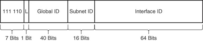
Figure 3-9 Unique Local Address Format
To use these addresses, an enterprise engineer would choose a 40-bit global ID in a pseudorandom manner rather than asking for a registered public prefix from an ISP or other registry. To form the complete prefix, the chosen 40 bits would be combined with the initial required 8 bits (hex FD) to form a 48-bit site prefix. The engineer can then use a 16-bit subnet field to create subnets, leaving a 64-bit interface ID. The interface ID could be created by static configuration or by the EUI-64 calculation.
This type of unicast address gives the engineer the ability to create the equivalent of an IPv4 private address structure, but given the huge number of available public IPv6 addresses, it might be more likely that engineers plan to use global unicast IP addresses throughout an enterprise.
Link-local Unicast Addresses
IPv6 uses link-local addresses for sending and receiving IPv6 packets on a single subnet. Many such uses exist; here’s just a small sample:
![]() Used as the source address for RS and RA messages for router discovery (as previously shown in Figure 3-7)
Used as the source address for RS and RA messages for router discovery (as previously shown in Figure 3-7)
![]() Used by Neighbor Discovery (the equivalent of ARP for IPv6)
Used by Neighbor Discovery (the equivalent of ARP for IPv6)
![]() Used as the next-hop IPv6 address for IP routes
Used as the next-hop IPv6 address for IP routes
By definition, routers use a link-local scope for packets sent to a link-local IPv6 address. The term link-local scope means exactly that—the packet should not leave the local link, or local subnet if you will. When a router receives a packet destined for such a destination address, the router does not forward the packet.
The link-local IPv6 addresses also help solve some chicken-and-egg problems, because each host, router interface, or other device can calculate its own link-local IPv6 address without needing to communicate with any other device. So, before sending the first packets, a host can calculate its own link-local address. Therefore, the host has an IPv6 address to use when doing its first overhead messages. For example, before a host sends an NDP RS (Router Solicitation) message, the host will have already calculated its link-local address, which can be used as the source IPv6 address in the RS message.
Link-local addresses come from the FE80::/10 range, meaning that the first 10 bits must be 1111 1110 10. An easier range to remember is that all hex link-local addresses begin with FE8, FE9, FEA, or FEB. However, practically speaking, for link-local addresses formed automatically by a host (rather than through static configuration), the address always starts with FE80, because the automatic process sets bits 11-64 to binary 0s. Figure 3-10 shows the format of the link-local address format under the assumption that the host or router is deriving its own link-local address, therefore using 54 binary 0s after the FE80::/10 prefix.

Figure 3-10 Link-local Address Format
IPv6 Unicast Address Summary
You might come across a few other types of IPv6 addresses in other reading. For example, earlier IPv6 RFCs defined the site local address type, which was meant to be used like IPv4 private addresses. However, this address type has been deprecated (RFC 3879). Also, IPv6 migration and coexistence tools use some conventions for IPv6 unicast addresses such that IPv4 addresses are embedded in the IPv6 address.
Additionally, it is helpful to know about other special unicast addresses. An address of all hex 0s, written ::/128, represents an unknown address. This can be used as a source IPv6 address in packets when a host has no suitable IPv6 address to use. The address ::1/128, representing an address of all hex 0s except a final hex digit 1, is a loopback address. Packets sent to this address will be looped back up the TCP/IP stack, allowing easier software testing. (This is the equivalent of IPv4’s 127.0.0.1 loopback address.)
Table 3-8 summarizes the IPv6 unicast address types for easier study.
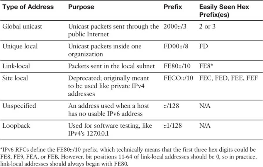
Table 3-8 Common IPv6 Unicast Address Types
Multicast and Other Special IPv6 Addresses
IPv6 supports multicasts on behalf of applications and multicasts to support the inner workings of IPv6. To aid this process, IPv6 defines ranges of IPv6 addresses and an associated scope, with the scope defining how far away from the source of the packet the network should forward a multicast.
All IPv6 multicast addresses begin with FF::/8. In other words, they begin with FF as their first two digits. Multicasts with a link-local scope, like most of the multicast addresses referenced in this chapter, begin with FF02::/16; the 2 in the fourth hex digit identifies the scope as link-local. A fourth digit of hex 5 identifies the broadcast as having a site local scope, with those multicasts beginning with FF05::/16.
For reference, Table 3-9 lists some of the more commonly seen IPv6 multicast addresses. Of particular interest are the addresses chosen for use by Routing Information Protocol (RIP), Open Shortest Path First (OSPF), and Enhanced IGRP (EIGRP), which somewhat mirror the multicast addresses that each protocol uses for IPv4. Note also that all but the last two entries have a link-local scope.
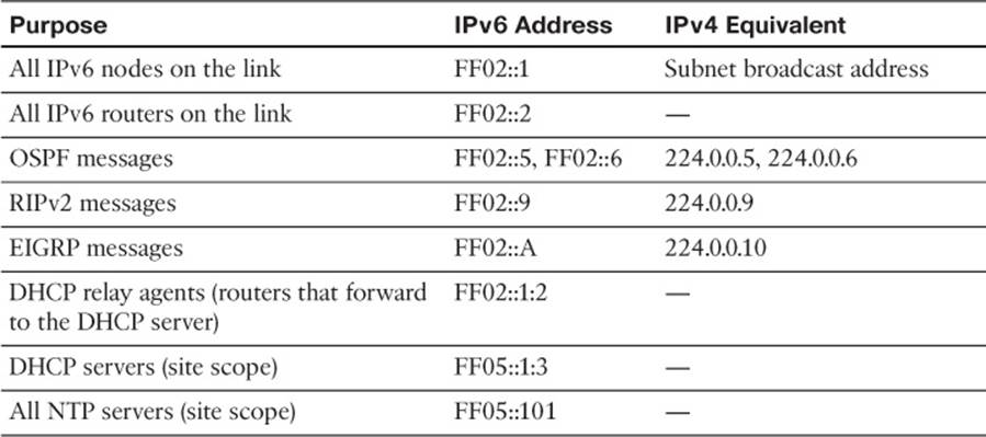
Table 3-9 Common Multicast Addresses
Layer 2 Addressing Mapping and Duplicate Address Detection
As with IPv4, any device running IPv6 needs to determine the data link layer address used by devices on the same link. IPv4 uses Address Resolution Protocol (ARP) on LANs and Inverse ARP (InARP) on Frame Relay. IPv6 defines a couple of new protocols that perform the same function. These new functions use ICMPv6 messages and avoid the use of broadcasts, in keeping with IPv6’s avoidance of broadcasts. This section gives a brief explanation of each protocol.
Neighbor Discovery Protocol for Layer 2 Mapping
When an IPv6 host or router needs to send a packet to another host or router on the same LAN, the host/router first looks in its neighbor database. This database contains a list of all neighboring IPv6 addresses (addresses on connected links) and their corresponding MAC addresses. If not found, the host or router uses the Neighbor Discovery Protocol (NDP) to dynamically discover the MAC address.
Figure 3-11 shows a sample of such a process, using the same host and router seen earlier in Figure 3-8.
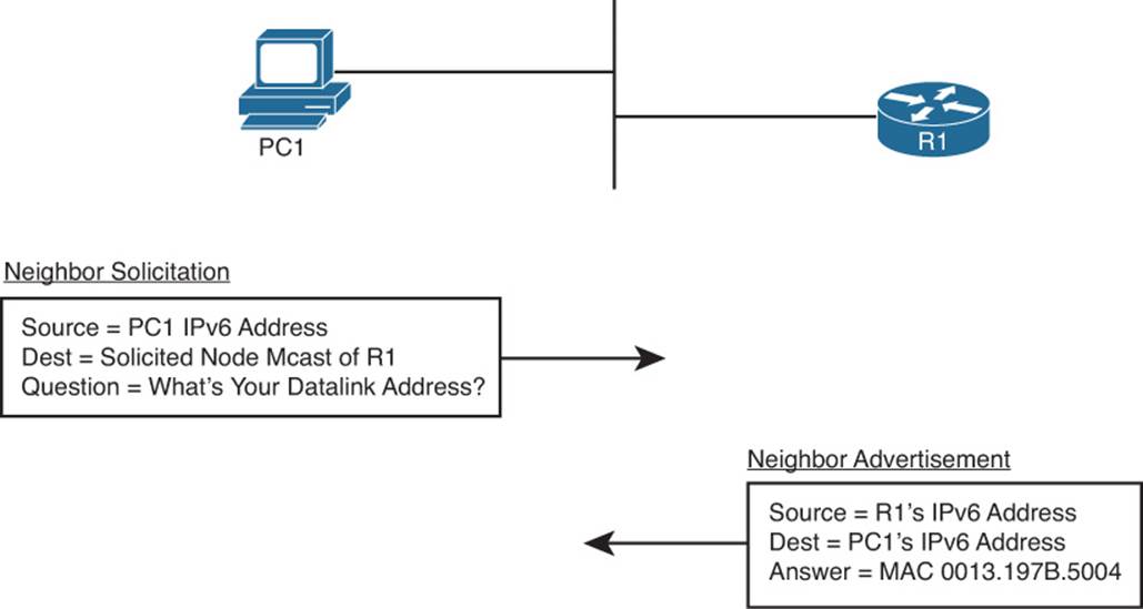
Figure 3-11 Neighbor Discovery Protocol
The process acts like the IPv4 ARP process, just with different details. In this case, PC1 sends a multicast message called a Neighbor Solicitation (NS) Internet Control Message Protocol (ICMP) message, asking R1 to reply with R1’s MAC address. R1 sends a Neighbor Advertisement (NA)ICMP message, which is unicast back to PC1, listing R1’s MAC address. Now PC1 can build a data-link frame with R1’s MAC listed as the destination address and send encapsulated packets to R1.
The NS message uses a special multicast destination address called a solicited node multicast address. On any given link, the solicited node multicast address represents all hosts with the same last 24 bits of their IPv6 addresses. By sending packets to the solicited node multicast address, the packet reaches the correct host, but it might also reach a few other hosts—which is fine. (Note that packets sent to a solicited node multicast address have a link-local scope.)
The solicited node multicast address begins with FF02::1:FF00:0/104. The final 24 bits (6 hex digits) of the address are formed by adding the last 24 bits of the IPv6 address to which the message is being sent. All IPv6 hosts listen for frames sent to their own solicited node multicast address, so that when a host or router receives such a multicast, the host realizes that it should reply. For example, in this case, based on R1’s IPv6 address previously seen in Figure 3-7
![]() R1’s IPv6 address: 2340:1111:AAAA:1:213:19FF:FE7B:5004
R1’s IPv6 address: 2340:1111:AAAA:1:213:19FF:FE7B:5004
![]() R1’s solicited node address: FF02::1:FF7B:5004
R1’s solicited node address: FF02::1:FF7B:5004
Note
The corresponding Ethernet multicast MAC address would be 0100.5E7B.5004.
Duplicate Address Detection (DAD)
When an IPv6 interface first learns an IPv6 address, or when the interface begins working after being down for any reason, the interface performs Duplicate Address Detection (DAD). The purpose of this check is to prevent hosts from creating problems by trying to use the same IPv6 address already used by some other host on the link.
To perform such a function, the interface uses the same NS message shown in Figure 3-11 but with small changes. To check its own IPv6 address, a host sends the NS message to the solicited node multicast address based on its own IPv6 address. If some host sends a reply, listing the same IPv6 address as the source address, the original host has found that a duplicate address exists.
Inverse Neighbor Discovery
The ND protocol discussed in this section starts with a known neighbor’s IPv6 address and seeks to discover the link-layer address used by that IPv6 address. On Frame Relay networks, and with some other WAN data-link protocols, the order of discovery is reversed. A router begins with knowledge of the neighbor’s data link layer address and instead needs to dynamically learn the IPv6 address used by that neighbor.
IPv4 solves this discovery problem on LANs using ARP and the reverse problem over Frame Relay using Inverse ARP (InARP). IPv6 solves the problem on LANs using ND, and now for Frame Relay, IPv6 solves this problem using Inverse Neighbor Discovery (IND). IND, also part of the ICMPv6 protocol suite, defines an Inverse NS (INS) and Inverse NA (INA) message. The INS message lists the known neighbor link-layer address (Data-Link Connection Identifier [DLCI] for Frame Relay), and the INS asks for that neighboring device’s IPv6 addresses. The details inside the INS message include the following:
![]() Source IPv6: IPv6 unicast of sender
Source IPv6: IPv6 unicast of sender
![]() Destination IPv6: FF02::1 (all IPv6 hosts multicast)
Destination IPv6: FF02::1 (all IPv6 hosts multicast)
![]() Link-layer addresses
Link-layer addresses
![]() Request: Please reply with your IPv6 address(es)
Request: Please reply with your IPv6 address(es)
The IND reply lists all the IPv6 addresses. As with IPv4, the show frame-relay map command lists the mapping learned from this process.
Configuring IPv6 Addresses on Cisco Routers
Most IPv6 implementation plans make use of both static IPv6 address configuration and dynamic configuration options. As is the case with IPv4, the plan assigns infrastructure devices with static addresses, with client hosts using one of the two dynamic methods for address assignment.
IPv6 addressing includes many more options than IPv4, and as a result, many more configuration options exist. A router interface can be configured with a static global unicast IPv6 address, either with or without using the EUI-64 option. Although less likely, a router could be configured to dynamically learn its IPv6 address with either stateful DHCP or stateless autoconfig. The router interface could be configured to either not use a global unicast address, instead relying solely on its link-local address, or to borrow another interface’s address using the IPv6 unnumbered feature.
This section summarizes the address configuration commands and shows several examples of configuration and verification commands for IPv6. To that end, Table 3-10 summarizes the IPv6 configuration commands and their meanings.
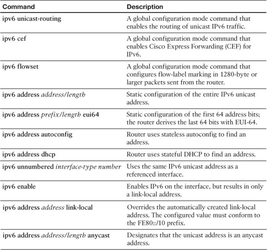
Table 3-10 Router IOS IPv6 Configuration Command Reference
Note
All the interface subcommands in Table 3-10 enable IPv6 on an interface, which means that a router derives an IPv6 link-local address for the interface. The description shows what the command does in addition to enabling IPv6.
Configuring Static IPv6 Addresses on Routers
The configuration examples in this section use the internetwork shown in Figure 3-12. The figure shows a diagram that you might see in an implementation plan, with the five IPv6 subnet numbers shown over the five links. The interface ID of each interface is then abbreviated, or shown as EUI-64, as a reminder of whether to configure the entire 128-bit address or to rely on the EUI-64 feature.
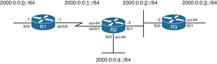
Figure 3-12 Sample IPv6 Address Planning Diagram
Example 3-1 shows the configuration process on Router R2, which uses EUI-64 on two interfaces and a complete IPv6 address on another. Also, note that the configuration includes the ipv6 unicast-routing global configuration command, which enables the router to route IPv6 traffic. (The addresses can be configured without also configuring ipv6 unicast-routing, but without this command, the router acts more like an IPv6 host, and it will not forward IPv6 packets.)
Example 3-1 R2’s IPv6 Configuration
R2# show running-config
! lines omitted for brevity
interface FastEthernet0/0
ipv6 address 2000:0:0:4::/64 eui-64
!
interface FastEthernet0/1
ipv6 address 2000:0:0:2::2/64
!
interface Serial0/0/1
ipv6 address 2000:0:0:1::/64 eui-64
!
!
R2# show ipv6 interface brief
FastEthernet0/0 [up/up]
FE80::213:19FF:FE7B:5004
2000::4:213:19FF:FE7B:5004
FastEthernet0/1 [up/up]
FE80::213:19FF:FE7B:5005
2000:0:0:2::2
Serial0/0/0 [administratively down/down]
unassigned
Serial0/0/1 [up/up]
FE80::213:19FF:FE7B:5004
2000::1:213:19FF:FE7B:5004
Serial0/1/0 [administratively down/down]
unassigned
Serial0/1/1 [administratively down/down]
unassigned
R2# show interfaces fa0/0
FastEthernet0/0 is up, line protocol is up
Hardware is Gt96k FE, address is 0013.197b.5004 (bia 0013.197b.5004)
MTU 1500 bytes, BW 100000 Kbit/sec, DLY 100 usec,
reliability 255/255, txload 1/255, rxload 1/255
! lines omitted for brevity
The ipv6 address commands both enable IPv6 on the associated interfaces and define either the prefix (with the EUI-64 option) or the entire address. The show commands listed after the configuration confirm the IPv6 addresses. Of particular note:
![]() All three interfaces now have link-local addresses that begin with FE80.
All three interfaces now have link-local addresses that begin with FE80.
![]() Fa0/1 has the address exactly as configured.
Fa0/1 has the address exactly as configured.
![]() S0/0/1 and Fa0/0 have the configured prefixes (2000:0:0:1 and 2000:0:0:4, respectively), but with EUI-64-derived interface IDs.
S0/0/1 and Fa0/0 have the configured prefixes (2000:0:0:1 and 2000:0:0:4, respectively), but with EUI-64-derived interface IDs.
![]() S0/0/1 uses Fa0/0’s MAC address (as shown in the show interfaces fa0/0 command) when forming its EUI-64.
S0/0/1 uses Fa0/0’s MAC address (as shown in the show interfaces fa0/0 command) when forming its EUI-64.
On this last point, whenever Cisco IOS needs a MAC address for an interface, and that interface does not have a built-in MAC address, the router uses the MAC address of the lowest-numbered LAN interface on the router—in this case, Fa0/0. The following list shows the derivation of the last 64 bits (16 hexadecimal digits) of R2’s IPv6 interface IDs for its global unicast IPv6 addresses on Fa0/0 and S0/0/1:
Step 1. Use Fa0/0’s MAC address: 0013.197B.5004.
Step 2. Split and insert FFFE: 0013:19FF:FE7B:5004.
Step 3. Invert bit 7: Hex 00 = 00000000 binary, flip for 00000010, and convert back to hex 02, resulting in 0213:19FF:FE7B:5004.
Multicast Groups Joined by IPv6 Router Interfaces
Next, consider the deeper information held in the show ipv6 interface fa0/0 command output on Router R2, as shown in Example 3-2. Not only does it list the same link-local and global unicast addresses, but it also lists other special addresses as well.
Example 3-2 All IPv6 Addresses on an Interface
R2# show ipv6 interface fa0/0
FastEthernet0/0 is up, line protocol is up
IPv6 is enabled, link-local address is FE80::213:19FF:FE7B:5004
No Virtual link-local address(es):
Global unicast address(es):
2000::4:213:19FF:FE7B:5004, subnet is 2000:0:0:4::/64 [EUI]
Joined group address(es):
FF02::1
FF02::2
FF02::1:FF7B:5004
MTU is 1500 bytes
ICMP error messages limited to one every 100 milliseconds
ICMP redirects are enabled
ICMP unreachables are sent
ND DAD is enabled, number of DAD attempts: 1
ND reachable time is 30000 milliseconds (using 22807)
ND advertised reachable time is 0 (unspecified)
ND advertised retransmit interval is 0 (unspecified)
ND router advertisements are sent every 200 seconds
ND router advertisements live for 1800 seconds
ND advertised default router preference is Medium
Hosts use stateless autoconfig for addresses.
The three joined multicast groups should be somewhat familiar after reading this chapter. The first multicast address, FF02::1, represents all IPv6 devices, so router interfaces must listen for packets sent to this address. FF02::2 represents all IPv6 routers, so again, R2 must listen for packets sent to this address. Finally, the FF02::1:FF beginning value is the range for an address’s solicited node multicast address, used by several functions, including Duplicate Address Detection (DAD) and Neighbor Discovery (ND).
Connected Routes and Neighbors
The third example shows some new concepts with the IP routing table. Example 3-3 shows R2’s current IPv6 routing table that results from the configuration shown in Example 3-1. Note that no IPv6 routing protocols have been configured, and no static routes have been configured.
Example 3-3 Connected and Local IPv6 Routes
R2# show ipv6 route
IPv6 Routing Table - Default - 7 entries
Codes: C - Connected, L - Local, S - Static, U - Per-user Static route
B - BGP, M - MIPv6, R - RIP, I1 - ISIS L1
I2 - ISIS L2, IA - ISIS interarea, IS - ISIS summary, D - EIGRP
EX - EIGRP external
O - OSPF Intra, OI - OSPF Inter, OE1 - OSPF ext 1, OE2 - OSPF ext 2
ON1 - OSPF NSSA ext 1, ON2 - OSPF NSSA ext 2
C 2000:0:0:1::/64 [0/0]
via Serial0/0/1, directly connected
L 2000::1:213:19FF:FE7B:5004/128 [0/0]
via Serial0/0/1, receive
C 2000:0:0:2::/64 [0/0]
via FastEthernet0/1, directly connected
L 2000:0:0:2::2/128 [0/0]
via FastEthernet0/1, receive
C 2000:0:0:4::/64 [0/0]
via FastEthernet0/0, directly connected
L 2000::4:213:19FF:FE7B:5004/128 [0/0]
via FastEthernet0/0, receive
L FF00::/8 [0/0]
via Null0, receive
First, the IPv6 routing table lists the expected connected and local routes. The connected routes occur for any unicast IPv6 addresses on the interface that happen to have more than link-local scope. So, R2 has routes for subnets 2000:0:0:1::/64, 2000:0:0:2::/64, and 2000:0:0:4::/64, but no connected subnets related to R2’s link-local addresses. The local routes, all /128 routes, are essentially host routes for the router’s unicast IPv6 addresses. These local routes allow the router to more efficiently process packets directed to the router itself, as compared to packets directed toward connected subnets.
The IPv6 Neighbor Table
The IPv6 neighbor table replaces the IPv4 ARP table, listing the MAC address of other devices that share the same link. Example 3-4 shows a debug that lists messages during the NDP process, a ping to R3’s Fa0/0 IPv6 address, and the resulting neighbor table entries on R2.
Example 3-4 Creating Entries and Displaying the Contents of R2’s IPv6 Neighbor Table
R2# debug ipv6 nd
ICMP Neighbor Discovery events debugging is on
R2# ping 2000:0:0:2::3
Type escape sequence to abort.
Sending 5, 100-byte ICMP Echos to 2000:0:0:2::3, timeout is 2 seconds:
!!!!!
Success rate is 100 percent (5/5), round-trip min/avg/max = 0/0/4 ms
R2#
*Sep 2 17:07:25.807: ICMPv6-ND: DELETE -> INCMP: 2000:0:0:2::3
*Sep 2 17:07:25.807: ICMPv6-ND: Sending NS for 2000:0:0:2::3 on FastEthernet0/1
*Sep 2 17:07:25.807: ICMPv6-ND: Resolving next hop 2000:0:0:2::3 on interface
FastEthernet0/1
*Sep 2 17:07:25.811: ICMPv6-ND: Received NA for 2000:0:0:2::3 on FastEthernet0/1
from 2000:0:0:2::3
*Sep 2 17:07:25.811: ICMPv6-ND: Neighbor 2000:0:0:2::3 on FastEthernet0/1 : LLA
0013.197b.6588
R2# undebug all
All possible debugging has been turned off
R2# show ipv6 neighbors
IPv6 Address Age Link-layer Addr State Interface
2000:0:0:2::3 0 0013.197b.6588 REACH Fa0/1
FE80::213:19FF:FE7B:6588 0 0013.197b.6588 REACH Fa0/1
The example shows the entire NDP process by which R2 discovers R3’s Fa0/0 MAC address. The example begins with a debug ipv6 nd command, which tells R2 to issue messages related to NDP messages. The ping 2000:0:0:2::3 command that follows tells Cisco IOS to use IPv6 to ping R3’s F0/0 address; however, R2 does not know the corresponding MAC address. The debug output that follows shows R2 sending an NS, with R3 replying with an NA message, listing R3’s MAC address.
The example ends with the output of the show ipv6 neighbor command, which lists the neighbor table entries for both of R3’s IPv6 addresses.
Stateless Autoconfiguration
The final example in this section demonstrates stateless autoconfiguration using two routers, R2 and R3. In Example 3-5, R2’s Fa0/1 configuration will be changed, using the ipv6 address autoconfig subcommand on that interface. This tells R2 to use the stateless autoconfig process, with R2 learning its prefix from Router R3. R2 then builds the rest of its IPv6 address using EUI-64.
Example 3-5 Using Stateless Autoconfig on Router R2
R2# conf t
Enter configuration commands, one per line. End with CNTL/Z.
R2(config)# interface fa0/1
R2(config-if)# no ipv6 address
R2(config-if)# ipv6 address autoconfig
R2(config-if)# ^Z
R2# show ipv6 interface brief
FastEthernet0/0 [up/up]
FE80::213:19FF:FE7B:5004
2000::4:213:19FF:FE7B:5004
FastEthernet0/1 [up/up]
FE80::213:19FF:FE7B:5005
2000::2:213:19FF:FE7B:5005
Serial0/0/0 [administratively down/down]
unassigned
Serial0/0/1 [up/up]
FE80::213:19FF:FE7B:5004
2000::1:213:19FF:FE7B:5004
Serial0/1/0 [administratively down/down]
unassigned
Serial0/1/1 [administratively down/down]
unassigned
R2# show ipv6 router
Router FE80::213:19FF:FE7B:6588 on FastEthernet0/1, last update 0 min
Hops 64, Lifetime 1800 sec, AddrFlag=0, OtherFlag=0, MTU=1500
HomeAgentFlag=0, Preference=Medium
Reachable time 0 (unspecified), Retransmit time 0 (unspecified)
Prefix 2000:0:0:2::/64 onlink autoconfig
Valid lifetime 2592000, preferred lifetime 604800
Starting with the configuration, the no ipv6 address command actually removes all configured IPv6 addresses from the interface and also disables IPv6 on interface Fa0/1. Then, the ipv6 address autoconfig command again enables IPv6 on Fa0/1 and tells R2 to use stateless autoconfig.
The show commands confirm that R2 does indeed learn its IPv6 address: 2000:0:0:2:0213:19FF:FE7B:5005. The show ipv6 router command, which lists the cached contents of any received RA messages, lists the information received from R3’s RA message, including R3’s link-local address (used to identify the routers) and R3’s advertised prefix (2000:0:0:2::/64).
RIP Next Generation (RIPng)
To support IPv6, all the IPv4 routing protocols had to go through varying degrees of changes, with the most obvious being that each had to be changed to support longer addresses and prefixes. The actual messages used to send and receive routing information have changed in some cases, using IPv6 headers instead of IPv4 headers, and using IPv6 addresses in those headers. In particular, like their IPv4 versions, each IPv6 IGP uses IPv6 multicast addresses. For example, RIPng sends routing updates to the IPv6 destination address FF02::9 instead of the old RIPv2 IPv4 224.0.0.9 address. Also, the routing protocols typically advertise their link local IP address as the next hop in a route.
Even with these changes, each IPv6 IGP has more similarities than differences compared to its respective IPv4 cousin. For example, RIPng, based on RIPv2, is still a distance vector protocol, with hop count as the metric and 15 hops as the longest valid route (16 is infinity). OSPF version 3 (OSPFv3), created specifically to support IPv6, uses link-state logic like OSPFv2, uses cost as the metric, and retains the link-state advertisement (LSA) types—but there are some changes to how the LSAs work. However, most of the core OSPF operational concepts remain the same. This section examines RIPng. Upcoming chapters examine OSPFv3 and EIGRP for IPv6.
Table 3-11 lists the IPv6 routing protocols and their new RFCs (as appropriate).
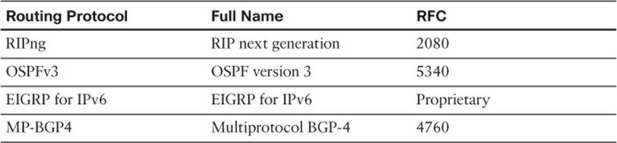
Table 3-11 Updates to Routing Protocols for IPv6
Routing Information Protocol (RIP) began life as one of the earliest efforts in the field of dynamic IP routing protocols. It eventually became the first dynamic routing protocol for the emerging IP protocol back in the 1970s. Later, in the mid-1990s, the RIP version 2 (RIPv2) specifications enhanced RIP, with the original version becoming known as RIP version 1, or simply RIPv1.
Also in the mid-1990s, the process of defining IPv6 was drawing toward completion, at least for the original IPv6 standards. To support IPv6, the IETF committees defined a new version of RIP to support IPv6. But rather than number this updated flavor of RIP as RIP version 3, the creators chose to number this new protocol as version 1, treating it like a new protocol. However, no one bothered to put “version 1” in the name, simply calling it RIP next generation (RIPng), or even simply RIP. To date, no new version of RIPng has been defined, making the original RIPng still the most recent version of the protocol.
Note
For you Star Trek TV show fans, yes, the name came in part from Star Trek: The Next Generation.
RIPng: Theory and Comparisons to RIPv2
The RIPng RFC states that the protocol uses many of the same concepts and conventions as the original RIPv1 specification, also drawing on some RIPv2 concepts. Table 3-12 lists a variety of facts about RIPv2 and RIPng.
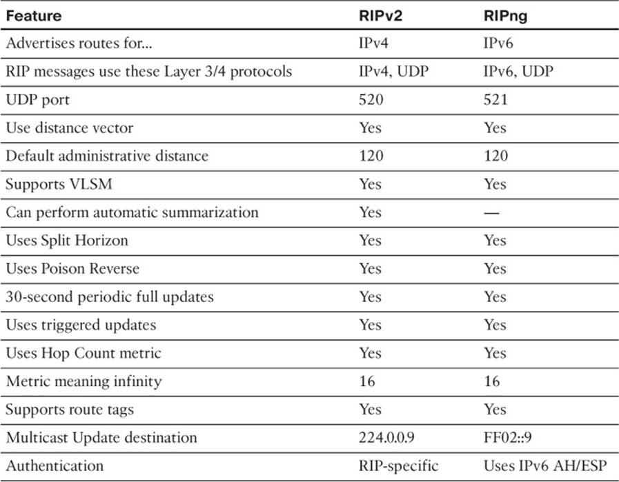
Table 3-12 Comparing RIPv2 to RIPng
The overall operation of RIPng closely matches RIPv2. In both, routers send periodic full updates with all routes, except for routes omitted because of Split Horizon rules. No neighbor relationships occur. The continuing periodic Updates, on a slightly variable 30-second period, also serve the purpose of confirming that the neighboring router still works. The metrics work exactly the same. When a router ceases to see a route in received updates, ceases to receive updates, or receives a poisoned (metric 16) route, it reacts to converge, but relatively slowly compared to EIGRP and OSPF.
Some differences relate specifically to IPv6. First, the messages themselves list IPv6 prefixes/lengths, rather than subnet/mask. In RIPv1 and RIPv2, RIP-encapsulated RIP Update messages inside an IPv4 and UDP header; with IPv6, the encapsulation uses IPv6 packets, again with a UDP header. Some small differences in the Update message format exist as well, with the most obvious difference being that the Updates list IPv6 prefixes and prefix lengths.
The last difference of note is that because IPv6 supports authentication using the IPsec Authentication Header (AH), RIPng does not natively support authentication, instead relying on IPsec.
Configuring RIPng
RIPng uses a new command style for the basic configuration, but most of the optional features and verification commands look much like the commands used for RIP for IPv4. This section first takes a look at the basic RIPng configuration, accepting as many defaults as possible.
The big difference between RIPv2 and RIPng configuration is that RIPng discards the age-old RIP network command in deference to the ipv6 rip name enable interface subcommand, which enables RIPng on an interface. Another difference relates to the routing of IPv4 and IPv6: Cisco IOS routes IPv4 by default (because of a default global configuration command of ip routing), but Cisco IOS does not route IPv6 by default (a default of no ipv6 unicast-routing). Finally, RIPng allows multiple RIPng processes on a single router, so Cisco IOS requires that each RIPng process is given a text name that identifies each RIPng process for that one router—another difference compared to RIPv2.
The following list shows the basic configuration steps for RIPng, including steps to enable IPv6 routing and enabling IPv6 on the interfaces:
Step 1. Enable IPv6 routing with the ipv6 unicast-routing global command.
Step 2. Enable RIPng using the ipv6 router rip name global configuration command. The name must be unique on a router but does not need to match on neighboring routers.
Step 3. Enable IPv6 on the interface, typically with one of these two methods:
![]() Configure an IPv6 unicast address on each interface using the ipv6 address address/prefix-length [eui-64] interface command.
Configure an IPv6 unicast address on each interface using the ipv6 address address/prefix-length [eui-64] interface command.
![]() Configure the ipv6 enable command, which enables IPv6 and causes the router to derive its link-local address.
Configure the ipv6 enable command, which enables IPv6 and causes the router to derive its link-local address.
Step 4. Enable RIP on the interface with the ipv6 rip name enable interface subcommand (where the name matches the ipv6 router rip name global configuration command).
The list includes just a few straightforward configuration commands, but a few subtle interactions also exist. The list shows steps related directly to RIPng (Steps 2 and 4), plus other steps related to making IPv6 itself work (Steps 1 and 3). The list also pairs two sets of dependent steps with each other, as follows:
![]() Step 2 relies on Step 1, because Cisco IOS rejects the command at Step 2 (ipv6 router rip name) if the command at Step 1 (ipv6 unicast-routing) has been omitted.
Step 2 relies on Step 1, because Cisco IOS rejects the command at Step 2 (ipv6 router rip name) if the command at Step 1 (ipv6 unicast-routing) has been omitted.
![]() Step 4 relies on Step 3, because Cisco IOS rejects the command at Step 4 if IPv6 has not yet been enabled on the interface.
Step 4 relies on Step 3, because Cisco IOS rejects the command at Step 4 if IPv6 has not yet been enabled on the interface.
Finally, note that although the ipv6 rip process-name enable interface subcommand (Step 4) refers to the process name configured at Step 2 (the ipv6 router rip process-name command), Cisco IOS creates the RIP process in reaction to the ipv6 rip process-name enable interface subcommand if that RIPng process name does not yet exist. In other words, if you followed the previous steps in order, but forgot to do Step 2, the command at Step 4 causes Cisco IOS to automatically create the command at Step 2.
As with RIPv1 and RIPv2, for any interface on which RIPng has been enabled, the RIP process does three main actions:
1. It starts sending RIP updates on that interface.
2. It also starts processing any RIP updates received on that interface.
3. Finally, it advertises the connected routes on that interface. In particular, because IPv6 allows the configuration of multiple IPv6 unicast addresses on an interface, RIP advertises most IPv6 unicast prefixes associated with the interface. The notable exceptions are that RIP does not advertise any link-local addresses, nor does RIP advertise the local host routes—routes with a /128 prefix length—created for each interface IPv6 address. In short, RIP advertises all routable subnets associated with the interface.
Figure 3-13 shows a sample internetwork with IPv6 global unicast IPv6 subnets displayed.
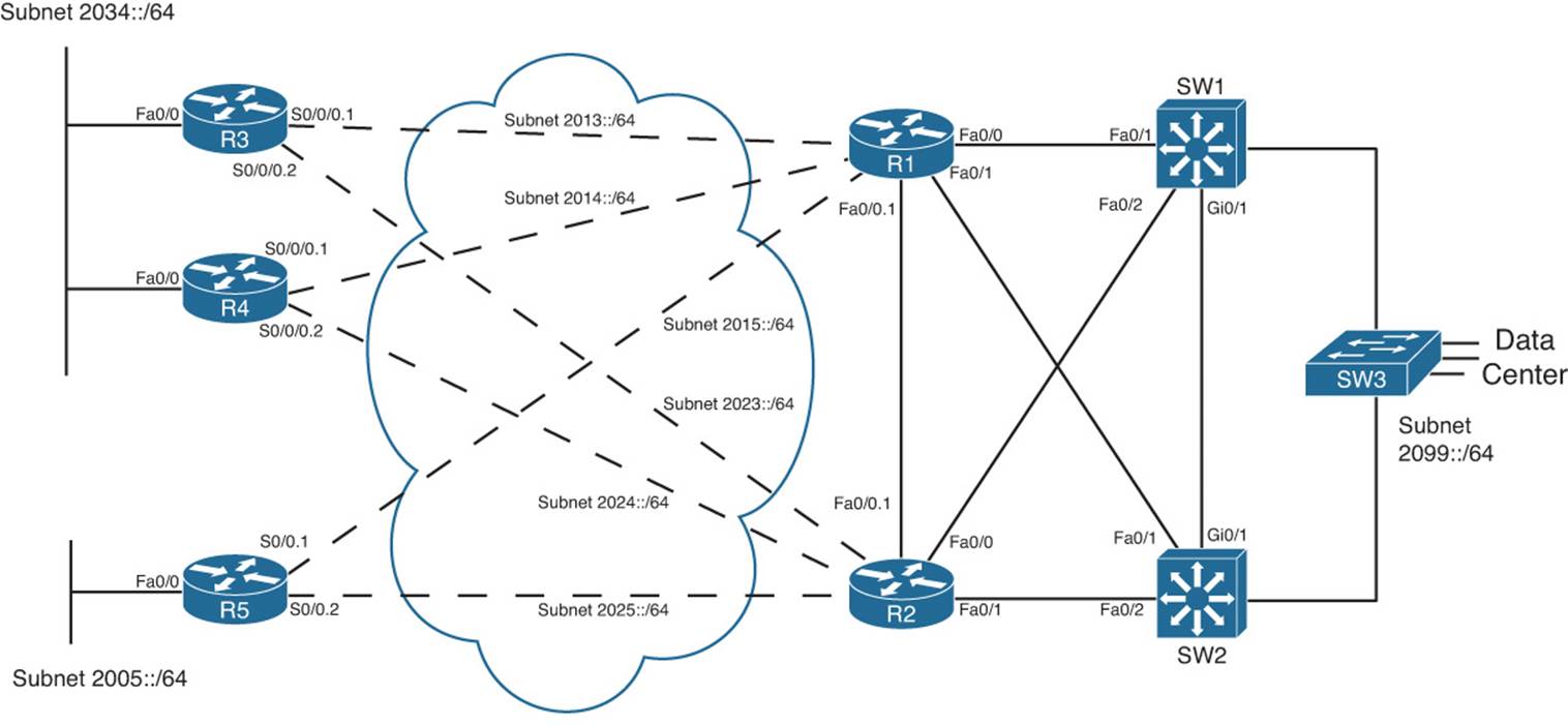
Figure 3-13 Sample Internetwork for IPv6 Routing Protocol Configuration
The sample internetwork uses addressing values that are both memorable and make for shorter IPv6 addresses when abbreviated. All the subnets use /64 prefix length, with quartets 2, 3, and 4 composed of all 0 values. The interface ID portion of each address uses all hex 0s in the first three quartets (quartets 5, 6, and 7 in the overall address), with the final digit in the final quartet used to identify each router. This last digit matches the name of each router in most cases.
For example, all of R1’s IPv6 addresses’ last four octets are 0000:0000:0000:0001. R1’s S0/0/0.3 subinterface, which connects with a permanent virtual circuit (PVC) to Router R3, uses a prefix of 2003:0000:0000:0000::/64, making the entire IPv6 address on this interface, when abbreviated, 2003::1/64—a convenient value for sifting through all the output in the upcoming examples.
Example 3-6 shows the RIPng configuration on Router R1 in this design. The RIP process name is fred.
Example 3-6 Configuring IPv6 Routing and Routing Protocols on R1
R1# show running-config
! The output is edited to remove lines not pertinent to this example.
! Next, step 1's task: enable IPv6 routing
ipv6 unicast-routing
!
! Next, on 5 interfaces, steps 3 and 4: configuring an IPv6 address,
! and enable RIPng, process "fred".
interface FastEthernet0/0.1
ipv6 address 2012::1/64
ipv6 rip fred enable
!
interface FastEthernet0/0.2
ipv6 address 2017::1/64
ipv6 rip fred enable
!
interface FastEthernet0/1.18
ipv6 address 2018::1/64
ipv6 rip fred enable
!
interface Serial0/0/0.3
ipv6 address 2013::1/64
ipv6 rip fred enable
!
interface Serial0/0/0.4
ipv6 address 2014::1/64
ipv6 rip fred enable
!
interface Serial0/0/0.5
ipv6 address 2015::1/64
ipv6 rip fred enable
!
! Next, step 2's task, creating the RIPng process named "fred"
ipv6 router rip fred
Verifying RIPng
The show commands related to RIPng have the same general kinds of information as seen with RIPv2. However, some of the commands used to get to the same piece of information differ, and of course, some obvious differences exist because of the different IPv6 address structure. Table 3-13 lists a cross-reference comparing all commands related to RIP that begin with either show ip or show ipv6. It also lists the similar debug commands used to display RIP routing information.
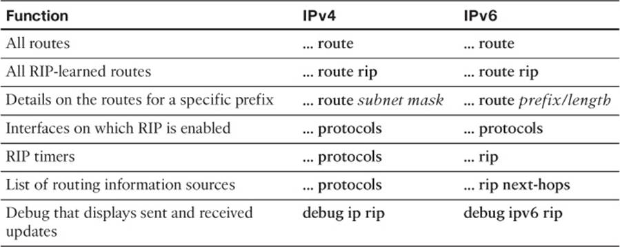
Table 3-13 Comparing Verification Commands: show ip and show ipv6
The most notable differences occur with the information seen with IPv4 in the show ip protocols command. The show ip protocols command displays a wide variety of information for IPv4 RIP, whereas the IPv6 commands spread the information over a couple of different commands, as listed in Table 3-13. Example 3-7 shows a sampling of the commands, taken from Router R3 in Figure 3-13. The explanatory comments are listed within the example in this case. Note that Router R3 used a RIPng process name of barney.
Example 3-7 IPv6 RIPng show Commands
! On R3, process name "barney" has two current routes to reach the
! datacenter prefix 2099::/64.
R3# show ipv6 route 2099::/64
Routing entry for 2099::/64
Known via "rip barney", distance 120, metric 3
Route count is 2/2, share count 0
Routing paths:
FE80::22FF:FE22:2222, Serial0/0/0.2
Last updated 00:27:12 ago
FE80::11FF:FE11:1111, Serial0/0/0.1
Last updated 00:27:10 ago
! Note that the next command lists only RIP-learned routes. It lists
! two next-hops for 2099::64. Note the next-hop information lists
! link-local addresses.
R3# show ipv6 route rip
IPv6 Routing Table - Default - 19 entries
Codes: C - Connected, L - Local, S - Static, U - Per-user Static route
B - BGP, M - MIPv6, R - RIP, I1 - ISIS L1
I2 - ISIS L2, IA - ISIS interarea, IS - ISIS summary, D - EIGRP
EX - EIGRP external
O - OSPF Intra, OI - OSPF Inter, OE1 - OSPF ext 1, OE2 - OSPF ext 2
ON1 - OSPF NSSA ext 1, ON2 - OSPF NSSA ext 2
R 2005::/64 [120/3]
via FE80::11FF:FE11:1111, Serial0/0/0.1
via FE80::22FF:FE22:2222, Serial0/0/0.2
R 2012::/64 [120/2]
via FE80::11FF:FE11:1111, Serial0/0/0.1
via FE80::22FF:FE22:2222, Serial0/0/0.2
! lines omitted for brevity...
R 2099::/64 [120/3]
via FE80::22FF:FE22:2222, Serial0/0/0.2
via FE80::11FF:FE11:1111, Serial0/0/0.1
! Unlike show ip protocols, show ipv6 protocols displays little info.
R3# show ipv6 protocols
IPv6 Routing Protocol is "connected"
IPv6 Routing Protocol is "rip barney"
Interfaces:
Serial0/0/0.2
Serial0/0/0.1
FastEthernet0/0
Redistribution:
None
! This command lists the timers displayed for RIPv2 with show ip protocols.
R3# show ipv6 rip
RIP process "barney", port 521, multicast-group FF02::9, pid 258
Administrative distance is 120. Maximum paths is 16
Updates every 30 seconds, expire after 180
Holddown lasts 0 seconds, garbage collect after 120
Split horizon is on; poison reverse is off
Default routes are not generated
Periodic updates 57, trigger updates 10
Interfaces:
Serial0/0/0.2
Serial0/0/0.1
FastEthernet0/0
Redistribution:
None
! This command lists the equivalent of the information in the
! show ip protocols commands' "Routing Information Sources" heading.
! Note the link-local addresses are listed.
R3# show ipv6 rip next-hops
RIP process "barney", Next Hops
FE80::11FF:FE11:1111/Serial0/0/0.1 [9 paths]
FE80::44FF:FE44:4444/FastEthernet0/0 [3 paths]
FE80::22FF:FE22:2222/Serial0/0/0.2 [9 paths]
Beyond the information emphasized in the comments inside the example, the next-hop IPv6 addresses in the example need to be scrutinized. RIPng uses the link-local IPv6 address as the next-hop IP address. (Reminder: link-local addresses begin with FE80.)
To discover which routers use which link-local addresses, and to make it easier to work with link-local addresses, you have a couple of options. First, you can set the MAC address of each LAN interface to something noticeable. For Example 3-7, the routers each used a recognizable MAC: R1 used 0200.1111.1111, R2 used 0200.2222.2222, and so on. Alternatively, you can just configure the link-local address with the ipv6 address command, using the link-local keyword at the end, and make each link-local address be more recognizable. Regardless, to find the router whose link-local address is listed in the IPv6 routing table, the show cdp entry name command can be useful, because it lists both the IPv4 and IPv6 addresses, including the neighbor’s link-local address.
Exam Preparation Tasks
Planning Practice
The CCNP ROUTE exam expects test takers to review design documents, create implementation plans, and create verification plans. This section provides some exercises that can help you to take a step back from the minute details of the topics in this chapter so that you can think about the same technical topics from the planning perspective.
For each planning practice table, simply complete the table. Note that any numbers in parentheses represent the number of options listed for each item in the solutions in Appendix F, “Completed Planning Practice Tables.”
Design Review Table
Table 3-14 lists several design goals related to this chapter. If these design goals were listed in a design document, and you had to take that document and develop an implementation plan, what implementation options come to mind? You should write a general description; specific configuration commands are not required.
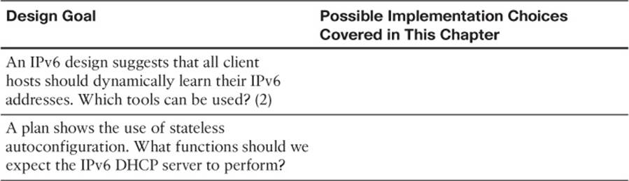
Table 3-14 Design Review
Implementation Plan Peer Review Table
Table 3-15 shows a list of questions that others might ask, or that you might think about, during a peer review of another network engineer’s implementation plan. Complete the table by answering the questions.
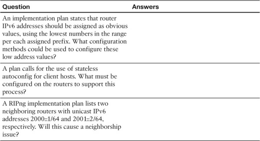
Table 3-15 Notable Questions from This Chapter to Consider During an Implementation Plan Peer Review
Create an Implementation Plan Table
To practice skills useful when creating your own implementation plan, list in Table 3-16 all configuration commands related to the configuration of the following features. You might want to record your answers outside the book, and set a goal to complete this table (and others like it) from memory during your final reviews before taking the exam.
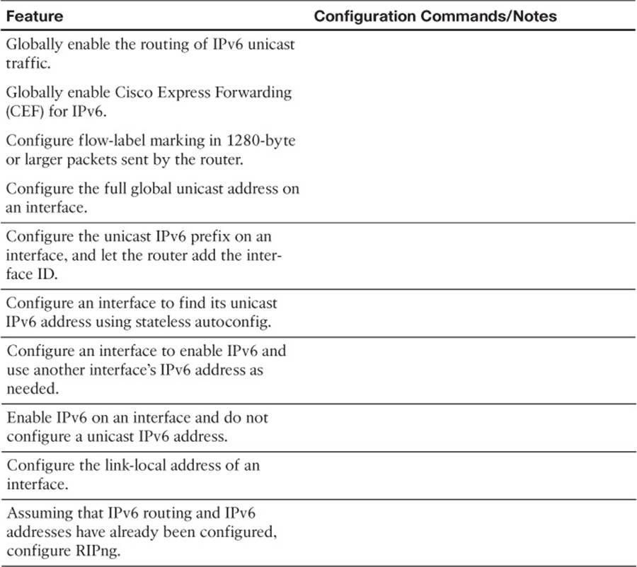
Table 3-16 Implementation Plan Configuration Memory Drill
Choose Commands for a Verification Plan Table
To practice skills useful when creating your own verification plan, list in Table 3-17 all commands that supply the requested information. You might want to record your answers outside the book, and set a goal to be able to complete this table (and others like it) from memory during your final reviews before taking the exam.
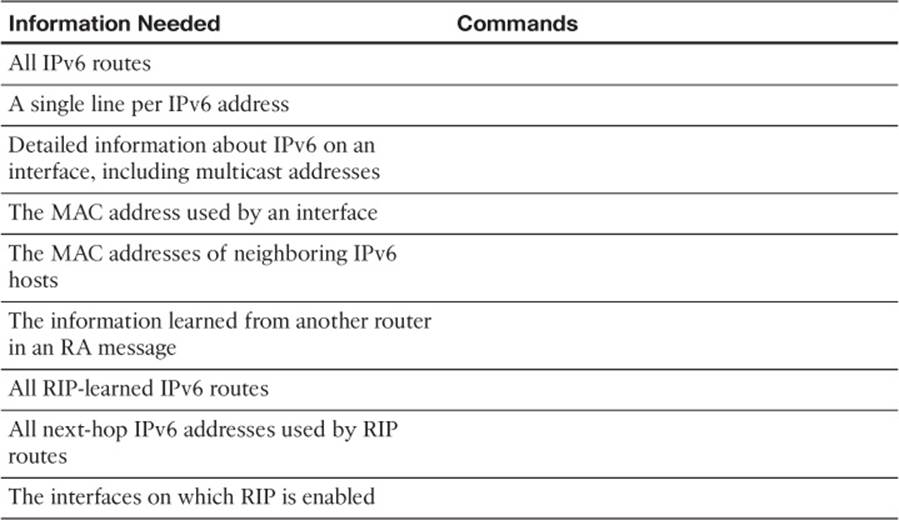
Table 3-17 Verification Plan Memory Drill
Note
Some of the entries in this table might not have been specifically mentioned in this chapter but are listed in this table for review and reference.
Review All the Key Topics
Review the most important topics from inside the chapter, noted with the Key Topic icon in the outer margin of the page. Table 3-18 lists a reference of these key topics and the page numbers on which each is found.
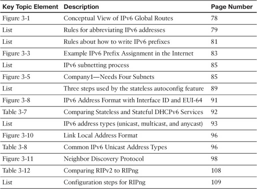
Table 3-18 Key Topics for Chapter 3
Complete the Tables and Lists from Memory
Print a copy of Appendix D, “Memory Tables,” (found on the CD) or at least the section for this chapter, and complete the tables and lists from memory. Appendix E, “Memory Tables Answer Key,” also on the CD, includes completed tables and lists to check your work.
Define Key Terms
Define the following key terms from this chapter, and check your answers in the glossary.
global unicast address
link-local address
unique local address
stateful DHCP
stateless DHCP
stateless autoconfig
Neighbor Discovery Protocol (NDP)
Neighbor Solicitation (NS)
Neighbor Advertisement (NA)
Router Solicitation (RS)
Router Advertisement (RA)
solicited node multicast address
Duplicate Address Detection (DAD)
Inverse Neighbor Discovery
RIP next generation (RIPng)