Juniper QFX5100 Series (2015)
Chapter 8. Overlay Networking
What is it and what problems can we solve with it?
These are the first questions that any good network engineer will ask when he first encounters a new technology or feature.
One of the larger problems in the data center is being able to easily orchestrate compute, storage, and networking to provide data center services with a click of a mouse. There are tools such as OpenStack, CloudStack, VMware vSphere and others that can help you accomplish this goal. The problem with these tools is that special plugins are required to help orchestrate the network. For example, if a new virtual machine (VM) was created and required to be on a separate network, the orchestration software would have to use a plugin to automatically configure the network switches with new Virtual Local Area Networks (VLANs), default gateways, and Access Control Lists (ACLs). The problem is that plugins only offer basic functionality and the feature parity varies between vendors. The other problem is that every time you create a new VM, add a NIC to an existing VM, or move a VM, it requires a change to the physical network.
One method of solving these problems is to decouple the virtual network from the physical network. The basic premise being that if all changes were made on the virtual networks, the physical network wouldn’t require changes. The tradeoff is that you’re moving complexity from one location to another. In this example, we’re moving physical network changes to a virtual concept. However, the benefit is that we can now abstract the way virtual networks are created, which reduces the operational complexity of the physical network. For example if you built a physical network with multiple vendors, the assumption is that no changes are required on the physical network when there’s a change to the virtual network. The benefit being that you don’t need to orchestrate network changes across a set of physical switches by different vendors; you simply worry about orchestrating change across the abstracted virtual network. Doing something the same way every time is much easier than doing the same thing with different styles. In a nutshell, overlay networking in the data center creates a hardware abstraction layer for the physical network and provides programmatic consistency.
Overlay networking might sound very similar to how physical servers were virtualized and abstracted from their underlying hardware. The basic premise is exactly the same. Virtualize the physical server and create a new virtual server that’s agnostic with respect to the underlying hardware. No need to worry about installing different operating system drivers to support different storage or networking cards. From the perspective of the VM, all of the operating system drivers are standardized, regardless if the underlying physical server uses solid-state drives (SSDs) or remotely mounted iSCSI targets. The same holds true for overlay networking in the data center. When you create a virtual network, it doesn’t have to worry about underlying protocols such as Spanning Tree Protocol (STP), Multi-Chassis Link Aggregation (MC-LAG), or Open Shortest Path First (OSPF).
As of this writing, overlay networking in the data center has started to trend and gain some adoption. The two primary options for data center overlay solutions are Juniper Contrail and VMware NSX. Each of these solutions creates virtual networks and decouples them from the physical hardware. You can orchestrate the virtual networks by using solutions such as OpenStack so that servers, storage, and networking are managed by a single tool.
Overview
As I mentioned in the introduction to this chapter, one of the key questions you should always ask when exploring a new piece of technology is what problem can you solve with it that you’re unable to solve today? If the answer is nothing new, the immediate follow-up question you should ask is does the new technology have a tangible benefit when compared with existing technology? The answer can come in multiple forms. For example, new technology might perform faster, have higher scale, or execute more quickly. If the new technology doesn’t offer any tangible benefits when compared with older technology, the industry refers to this as a “solution looking for a problem.”
So, what problem does overlay networking in the data center solve that can’t be solved today? The simple answer is that overlay networking gives you the capability to programmatically create logical networks in a standardized workflow without having to worry about the underlying hardware. Do you have a Juniper network? No problem, you can spin up logical networks using a standard Application Programming Interface (API). Do you have a Juniper network with other networking gear from other vendors? No problem. Use the same API to create logical networks.
There’s also another problem that exists in the data center. Standard access switches that are used as top-of-rack (ToR) switches are made by using merchant silicon (also referred to as “off-the-shelf silicon”) such as the Broadcom Trident 2 chipset. These switches have a limited Ternary Content Addressable Memory (TCAM) and can only scale so far in terms of MAC addresses, host entries, and IP address prefixes. Traditionally if you needed larger scale, you had to move away from merchant silicon and on to something that’s purpose built for high scale such as Juniper silicon. Two good examples of Juniper silicon are the Juniper MX routers and Juniper EX9200 switches; these products have much higher scale than their counterparts in the access switches. The problem is that you can’t use a Juniper MX or Juniper EX9200 as an access switch. Overlay networking moves the scale outside of the network and into the servers. All MAC addresses, host entries, and IP address prefixes are now stored in standard servers using x86 CPUs and large amounts of memory, which offer much greater scale than merchant silicon found in access switches.
Clearly, there are some unique benefits to overlay networking in the data center: standardized programmatic creation of logical networks and much higher scale are but two. How can you use these new advantages in a real-world use case? Two of the most popular use cases that benefit from overlay networking are IT-as-a-Service and Infrastructure-as-a-Service. Let’s take a look at each of these in more detail.
IT-as-a-Service
One of the most popular use cases for overlay networking is IT-as-a-Service (ITaaS), which you can see in Figure 8-1. The scenario is that a business would implement ITaaS so that internal corporate users could simply request IT resources through a self-service portal. The user would be presented with a menu of services such as the following:
§ Small VM: 1 core, 512 MB of memory, and 2 GB of storage
§ Medium VM: 2 cores, 2 GB of memory, and 10 GB of storage
§ Large VM: 4 cores, 8 GB of memory, and 50 GB of storage
The end user would select which item she wants from the menu of services and submit it into the self-service portal, as shown in the first step in Figure 8-1. The next step is that the self-service portal automatically creates the VM in the data center. The final step is that the VM is online and available to the user.
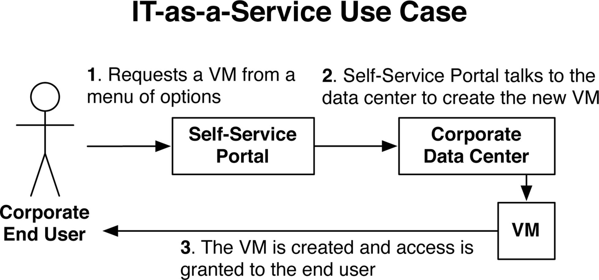
Figure 8-1. An ITaaS use case
The benefit is that end users can create, modify, and delete VMs without using a ticketing system that traditionally requires the work of three other people: a server administrator, a storage administrator, and a network engineer. When people are involved in the process, the time to create and deliver a VM back to the end user could take weeks. With ITaaS, the entire workflow is automated and the VM is delivered to the end user within minutes.
Infrastructure-as-a-Service
The second most common use case for overlay networking is Infrastructure-as-a-Service (IaaS). The scenario is that a service provider already has an existing MultiProtocol Label Switching (MPLS) network from which customers can buy transport services. The customers need a large WAN to interconnect their sites (see Figure 8-2). For example, the headquarters of Customer-1 is connected to his retail stores; and the headquarters of Customer-1 is connected to all of his branch offices. So far, this is a standard service provider offering around MPLS. The IaaS comes into play when the service provider offers managed VMs to customers over their existing MPLS transport. For example, Customer-3 can buy a VM from the service provider’s hosted data center and be able to access his private VM from his headquarters and data center. The same is true for Customer-1; she can buy a private VM from the service provider and access the VM directly from her retail stores through the service provider’s MPLS network, as illustrated in Figure 8-2.
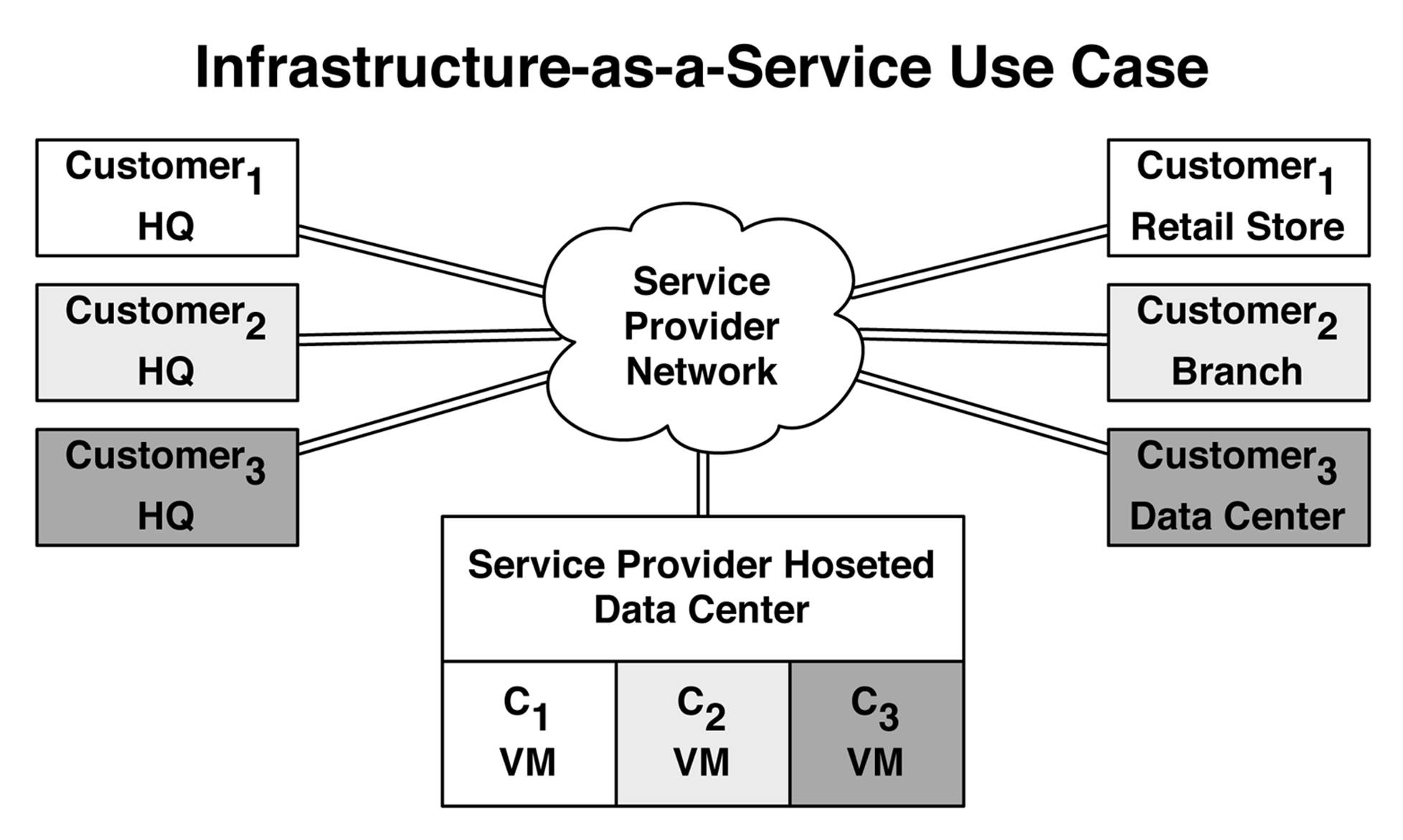
Figure 8-2. An IaaS use case
The benefit to the customers is that they can simply buy private VMs from the service provider and not have to worry about the underlying infrastructure. To make things even better, the customers can use their existing WAN connections from the service provider to access the VMs. Any customer locations such as headquarters, branch offices, or data centers that are connected into the service provider network will have connectivity to the VMs. The benefit to the service provider is that it can reuse its existing MPLS network to deliver new services to an existing customer base.
The Rise of IP Fabrics
There’s a fundamental shift in the way data centers are built when moving to an overlay network. Because the server traffic is encapsulated and transmitted through overlay tunnels, the networking requirements have been reduced to support only Layer 3. Even when two VMs require Layer 2 connectivity, you can do this through an overlay network between the two VMs; the only core requirement on the underlying network is to support Layer 3.
Building a data center network on top of a routed, Layer 3 network is inherently more stable because it only has to support a single routing protocol. The requirement for Layer 2 has been completely removed and you no longer need to worry about STP, MC-LAG, and other Layer 2 protocols. A pure Layer 3 network is also able to scale higher in terms of physical devices and logical routing. Each switch in the network can simply run a routing protocol with every other switch in the network and take advantage of full Equal-Cost Multipath (ECMP). Because each switch is in full Layer 3 mode, it doesn’t need to worry about propagating MAC addresses and can adjust its TCAM to support more Layer 3 entries.
Taking advantage of my personal experience in the data center, I’ve found that there’s an even split between traditional networks and Ethernet Fabrics in the enterprise market through tier-1 service providers (see Figure 8-3), with traditional networks being defined as a core switch running Layer 3, distribution switches running both Layer 2 and Layer 3, and the access switches in Layer 2 mode, and Ethernet Fabrics being defined as a solution such as Juniper QFabric and Virtual Chassis Fabric. As of this writing, only a small number of customers are moving toward IP Fabrics and overlay networks.
However, there is a segment of customers in the web-services market called Massively Scalable Data Centers (MSDC) that fully use IP Fabrics. Most of these customers do not virtualize their workloads and have no requirement for overlay networking. Instead, they have custom-written applications, built-in redundancy, and no requirement for Layer 2. The benefit being that large web-scale companies can build data centers that house 100,000s of servers and the application availability is very high.
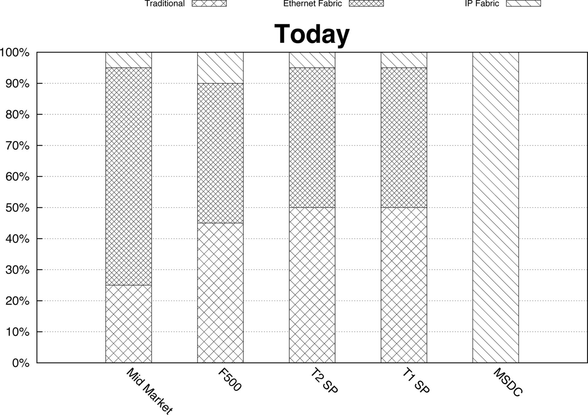
Figure 8-3. Network architectures mapped to customer segments as of August 2014
Given the benefits of overlay networking in the enterprise, it’s fully expected that as market adoption takes place, a larger percentage of enterprise customers will move toward an IP Fabric network architecture as depicted in Figure 8-4.
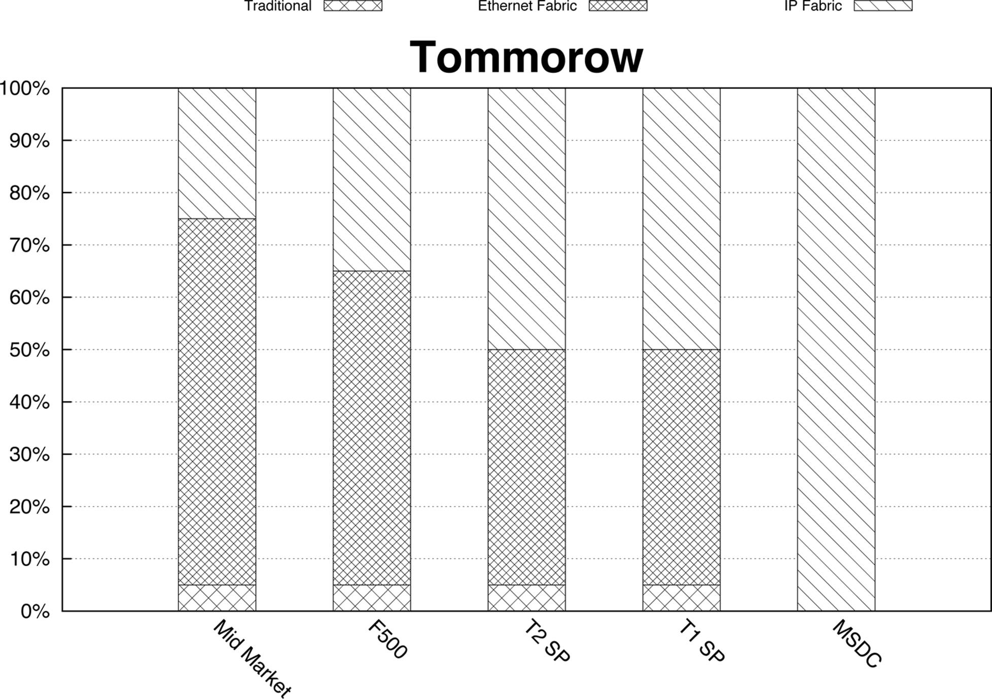
Figure 8-4. Network architectures mapped to customer segments—forecast for 2018
Today, there is a large percentage of enterprise and service-provider customers that are moving from a traditional network architecture to an Ethernet Fabric architecture, regardless of where overlay networking is going. The driving factors to use an Ethernet Fabric architecture is reduced operational complexity, storage convergence, and full support for Layer 2 and Layer 3 ECMP without depending on STP and MC-LAG.
To sum up, given the existing migration from traditional architectures to Ethernet Fabric architectures, plus the benefits of overlay architectures, it’s my assertion that within five years, there will be an even split between Ethernet Fabrics and IP Fabrics. There will be no change in the way the MSDC customers do business; it’s predicted that they will stay with an IP Fabric architecture and continue providing web-scale Software-as-a-Service (SaaS) applications.
Architecture
Overlay networking in the data center has many moving parts that are required to make it all work. The promise of being able to programmatically create virtual networks with standard APIs and not having to worry about the physical network isn’t an easy task. There are layers of abstraction that must work together to create a true end-to-end service offering to the network operator and end users.
The first thing to understand about overlay networking is that it gets its name from building overlay networks between the hypervisor hosts (see Figure 8-5). By creating overlay tunnels between hypervisor hosts, the underlying network simply needs to handle Layer 3 connectivity. Figure 8-5shows the entire data center network as a Layer 3 cloud. When VMs need to communicate with one another, the VM-to-VM traffic is encapsulated into an overlay tunnel and transmitted across the underlying Layer 3 network infrastructure until it reaches the destination hypervisor. The destination hypervisor receives the VM-to-VM traffic through the overlay tunnel, and it will decapsulate the traffic and forward it to the destination VM.
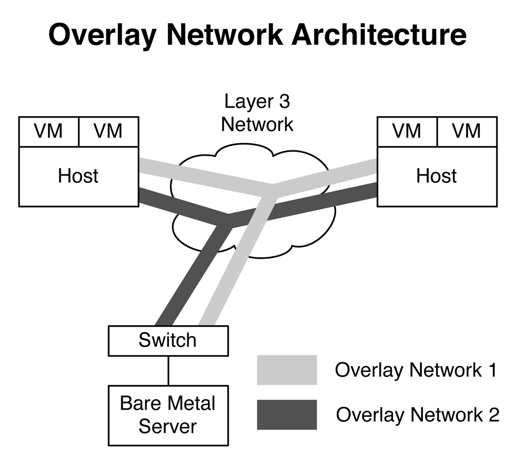
Figure 8-5. High-level architecture of overlay networking
Overlay networking works well when there’s nothing but VMs in your data center. The tricky part is how to handle nonvirtualized servers such as bare-metal servers and appliances. These servers expect to speak native Ethernet to the switch and do not have the benefit of a hypervisor handling the overlay tunnels on their behalf. The answer is that the access switch itself can handle the overlay tunnel encapsulation and forwarding on behalf of the nonvirtualized servers, as demonstrated in Figure 8-5. From the perspective of a bare-metal server, it simply speaks standard Ethernet to the access switch, and then the access switch handles the overlay tunnels. The end result is that both virtual and nonvirtualized servers can use the same overlay architecture in the data center.
Controller-Based Overlay Architecture
One of the most common types of overlay architectures includes the use of a controller. The basic premise being that all of the Virtual Tunnel End Points (VTEPs) are provisioned and MAC address learning is handled through a centralized controller. The benefit to a controller-based architecture is that the MAC address learning happens in the control plane, as opposed to the data plane, which is less efficient. A controller-based architecture also provides a single point of management for the provisioning of virtualized networks through the creation of tunnels and VTEPs. Let’s put all of the pieces together in a more detailed view of the end-to-end architecture for overlay networking. Figure 8-6 shows how virtualized and nonvirtualized servers are able to build overlay tunnels between the hypervisors and leaf switches.
All of the overlay tunnel end points are terminated in the host hypervisor or in the leaf switch. Notice that the overlay controller is connected to each tunnel end point. The controller handles the creation of overlay tunnels and MAC address learning. The overlay controller is connected to an overlay manager, which has a set of APIs. Cloud management software (CMS) such as OpenStack can use these APIs for network orchestration.
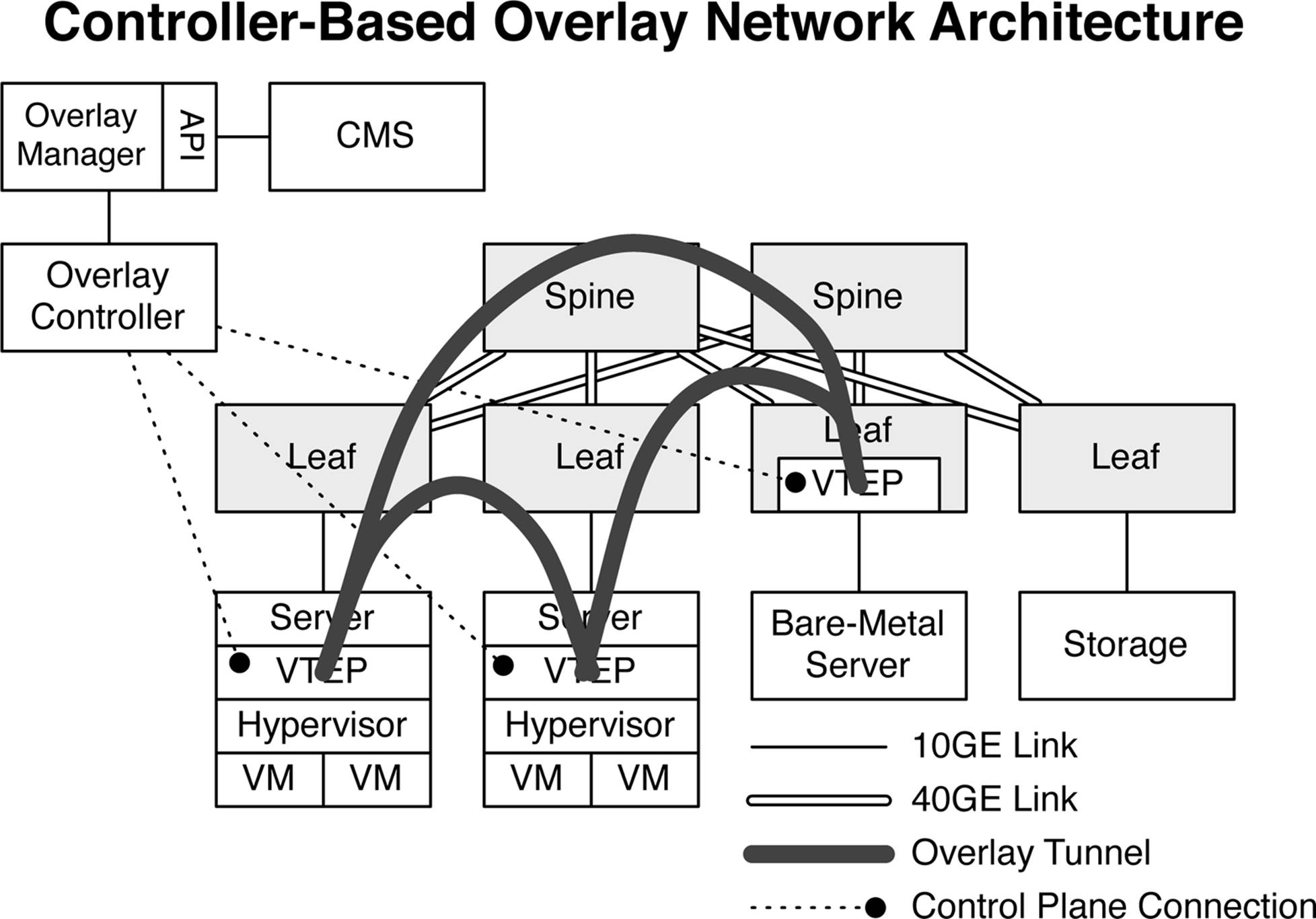
Figure 8-6. Controller-based overlay network architecture
Controller-Less Overlay Architecture
The alternative to a controller-based overlay architecture is a controller-less overlay architecture. The concept is that there is no centralized controller that’s handling the MAC address learning.
Multicast
In the original Virtual Extensible LAN (VXLAN) draft, it was suggested to use multicast between VTEPs to enable MAC address learning. Multicast would simulate an Ethernet switch and simply forward all broadcast and unknown unicast traffic to every other VTEP in the network. The end result is that MAC addresses are flooded to every port in the IP Fabric and MAC address learning happens in the data plane, as shown in Figure 8-7.
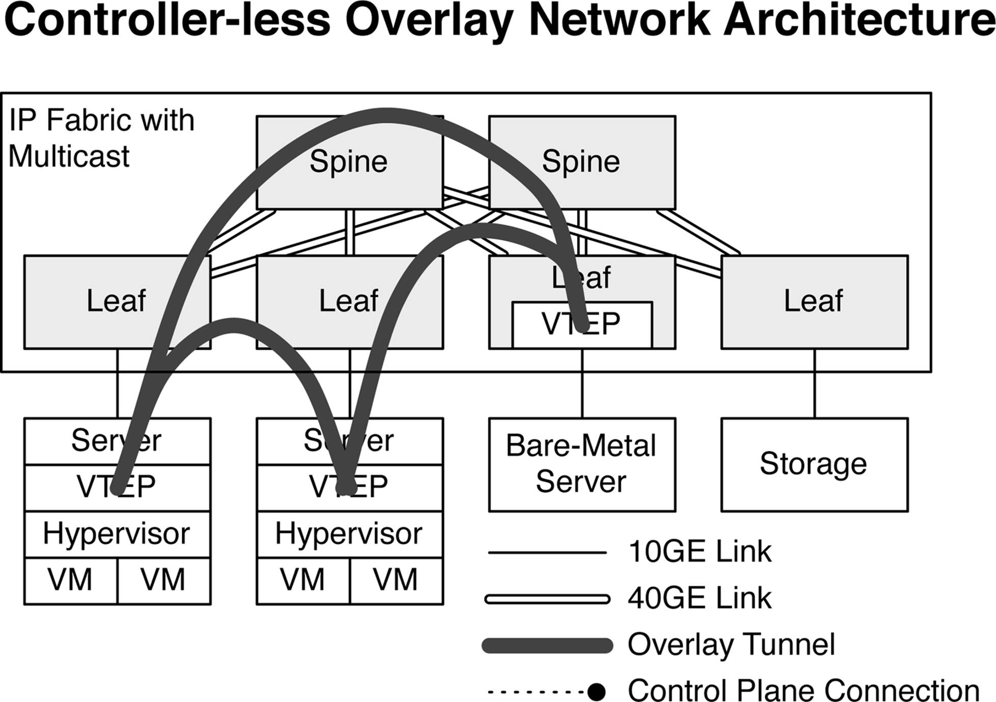
Figure 8-7. Controller-less overlay network architecture with multicast IP Fabric
The multicast option portrayed in Figure 8-7 is inefficient because it uses the data plane as a flooding mechanism for MAC address learning. It’s very common to have multiple VTEPs in a data center, but each VTEP will have different VXLAN memberships. For example a VTEP on Leaf-1 may have a VXLAN membership of VNI-1, VNI-2, and VNI-3; VTEP on Leaf-2 may have a VXLAN membership of VNI-2, VNI-3, and VNI-4. Using multicast in this scenario would send broadcast and unknown cast traffic for VNI-1 to Leaf-2, although Leaf-2 doesn’t have VNI-1 in the VTEP. The only way to work around this is to map VTEPs to a multicast group. However, this doesn’t scale very well, because sooner or later you run out of multicast groups. Besides, who wants to maintain a VTEP to multicast group mapping and have to continually update it?
EVPN
The alternative to using multicast in a controller-less overlay architecture is to use a control plane protocol such as EVPN. Most people think that Ethernet VPN (EVPN) is tied directly to MPLS VPNs, but Juniper has decoupled the EVPN control plane from the data plane. You can now couple the EVPN control plane protocol with any data plane encapsulation, such as VXLAN, as shown in Figure 8-8.
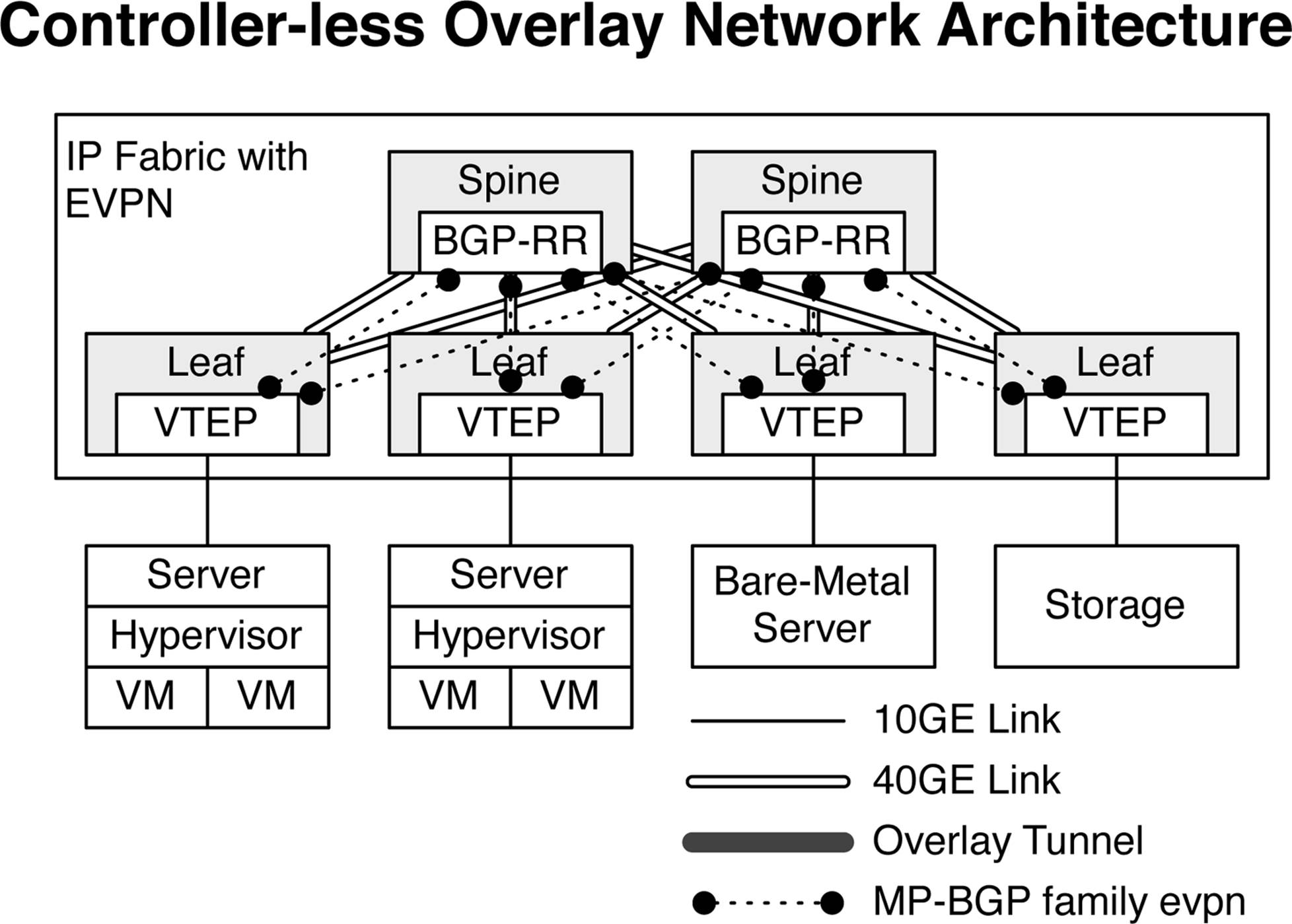
Figure 8-8. Controller-less overlay network architecture with IP Fabric and EVPN
EVPN is a very efficient control plane protocol because it uses standard Multiprotocol-Border Gateway Protocol (MP-BGP) extended communities such as route targets (RT) and route distinguishers (RD) to uniquely identify VTEP and VXLAN memberships. Now, VTEPs can exchange MAC addresses through EVPN with other VTEPs who are interested in specific VXLAN Network Identifiers (VNIs). The result is that MAC address learning is perfectly efficient when compared to multicast.
The controller-less overlay network architecture with EVPN is commonly referred to as a VXLAN Fabric. One of the other architectural changes in a VXLAN Fabric is that all of the VTEPs are now located in the networking equipment. The servers no longer need to worry about VTEPs and MAC address learning. All of the VXLAN switching, routing, and MAC address learning is handled by the networking equipment. From the perspective of the server, it’s simply Ethernet.
The inter-VXLAN routing is handled in the spine with hardware that uses Juniper silicon, such as the Trio chipset. As of this writing, there is no available merchant silicon from Broadcom that’s able to route VXLAN traffic. The default gateway of the servers is also handled by the spine switches, as illustrated in Figure 8-9.
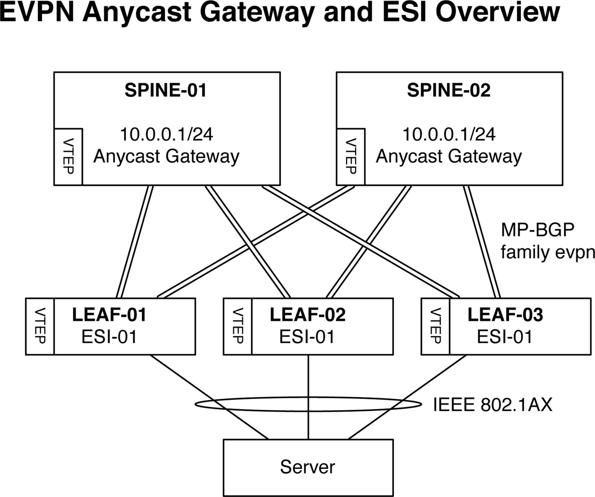
Figure 8-9. Illustration of EVPN Anycast gateway and ESI overview
The default gateway is synchronized with the EVPN protocol; each spine switch shares a common Anycast default gateway that’s able to route traffic from any server. For example, in Figure 8-9, the server’s default gateway would be 10.0.0.1. Also notice that the server is connected via LACP/IEEE 802.1AX to three switches: LEAF-01, LEAF-02, and LEAF-03. Depending on how the traffic is locally hashed within the server, the traffic can end up going to any of the three leaf switches. Because each of the three leaf switches share a common Ethernet Segment ID (ESI) for the server, each switch knows that any traffic that arrives from the server is part of the same virtual IEEE 802.1AX bundle.
EVPN has major benefits in a VXLAN Fabric architecture. The first is the reduction of wasted IP space for default gateways. Now, you can use the same IP address across a set of spine switches and serve as the Anycast default gateway for a particular broadcast domain. The second benefit is that EVPN allows a server to be multi-homed into the network, as opposed to dual-homed. The advantage is that EVPN can span more than two leaf switches to provide the ultimate link resiliency.
Traffic Profiles
Let’s take a look at the basic traffic patterns in an overlay network. It’s important to understand where data can originate and where it can be destined. Depending on what the source and destination end points are, different functional roles in the architecture are used to ensure that traffic is delivered end to end. Figure 8-7 shows that in an overlay architecture, there are three basic traffic patterns that can take place:
§ VM-to-VM traffic
§ VM-to–physical server traffic
§ Physical server–to–physical server traffic
Regardless of the traffic profile, the thing in common is that all traffic must pass through a VTEP. The VTEP is what terminates the tunnel at the source and destination of each overlay tunnel, as shown in Figure 8-10.
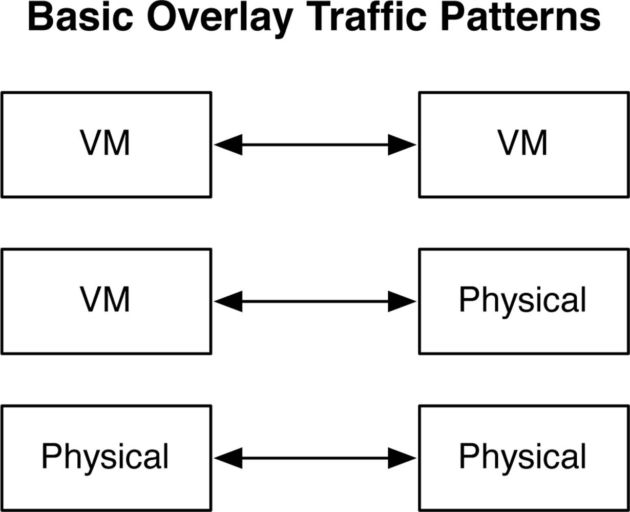
Figure 8-10. Basic overlay traffic patterns
VM-to-VM traffic will be handled by the VTEPs in the host hypervisor. The exception is that if a VM needs to communicate with a physical server, the traffic will still flow from VTEP to VTEP, but in this example, the host hypervisor VTEP will communicate with the access switch VTEP to handle the VM-to–physical server traffic. The final traffic profile is physical server–to–physical server. In this example, the traffic will be handled completely by access switch VTEPs at the source and at the destination. The end result is that regardless of the traffic profiles, overlay networking provides a seamless architecture to the network operator.
VTEPs
We already know that VTEPs terminate each end of an overlay tunnel. Let’s make a closer examination to see how they actually work. There are three primary functions for each VTEP, as shown in Figure 8-11.
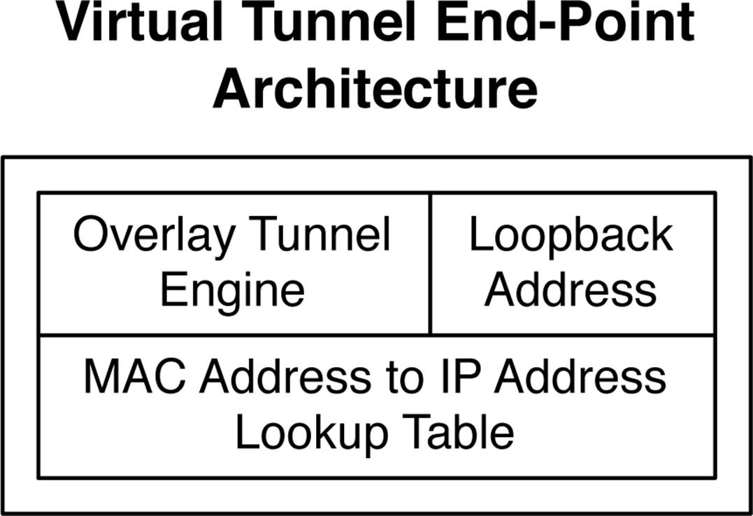
Figure 8-11. VTEP architecture
Overlay Tunnel Engine
As VMs and physical servers transmit and receive traffic, that traffic needs to be placed into and out of the overlay tunnel. As traffic enters the overlay tunnel it will be encapsulated with the data plane of choice, which is typically VXLAN. When the traffic exits the other end of the tunnel, the overlay data plane needs to be removed and forwarded to the destination server.
Loopback Address
As traffic is transmitted across an overlay tunnel, it requires a source and destination VTEP address. The loopback address provides the VTEP with Layer 3 reachability to other VTEPs in the network. Because VTEPs only require Layer 3 reachability between each other, this removes the underlying requirement for Layer 2 in the physical network.
MAC Address–to–IP Address Lookup Table
One of the most critical roles of the VTEP is its ability to learn MAC addresses and map them to IP addresses and VTEP addresses. If MAC-1 was learned by VTEP-1, how would VTEP-2 know to forward any traffic with a destination address of MAC-1 to VTEP-1? The answer is that each VTEP has a global table of every MAC address in the network and which VTEP and IP address with which it’s associated.
MAC address learning takes place inside the hypervisor or access switch and is replicated within each local VTEP. For every MAC address learned, its associated IP address and local VTEP loopback address is populated into a VTEP table, as illustrated in Figure 8-12.
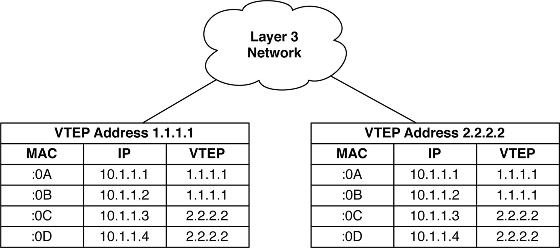
Figure 8-12. VTEP MAC, IP, and loopback tables
Each VTEP knows all local and remote MAC addresses and IP addresses. For example, if VTEP 1.1.1.1 wanted to send traffic to a destination VM with a MAC address ending in :0A, it knows that the VM is local and can simply perform local forwarding. However if VTEP 1.1.1.1 wanted to send traffic to a destination VM with the MAC address ending in :0D, it knows that the VM is owned by the VTEP with the address of 2.2.2.2. In this case, VTEP 1.1.1.1 would encapsulate the traffic destined to the MAC address ending in :0D in an overlay tunnel that was destined to the VTEP address 2.2.2.2 and transmit it over Layer 3. The destination VTEP 2.2.2.2 receives the encapsulated traffic and removes the overlay encapsulation. It inspects the destination MAC address and sees that :0D is a local MAC address and simply forwards the traffic to the VM. The same function is performed for both VMs and physical servers attached to access switches that have VTEPs.
Broadcom Trident II VTEPs
One caveat regarding the Broadcom Trident II VTEP is that it only maps MAC addresses to interfaces. This is because it’s unable to route VXLAN traffic; it can only forward it across Layer 2. The end result is that something besides a Broadcom Trident II VTEP is required to route VXLAN traffic. Here are three alternatives:
Juniper Silicon
Juniper switches such as the EX9200, and routers such as the MX series use custom-built Juniper silicon called the Trio chipset. These platforms make it possible for you to bind the MAC address, interface, and IP address within the chipset. The end result is that you can both switch and route VXLAN traffic.
Hypervisor VTEP
VTEPs that reside within a hypervisor such as Linux KVM have a specialized function called a virtual router (vRouter). These vRouters are able to map the MAC addresses, interfaces, and IP addresses into tables in the hypervisor, which allow it to switch and route VXLAN traffic.
Custom Appliances
The same principle applies, except the VXLAN routing is handled by a specialized piece of hardware in an appliance form factor. This option isn’t very popular, but does exist.
Control Plane
Depending on the overlay solution used, there are various types of control plane options. At a high level, there are two methods to take care of MAC address learning between VTEPs: multicast and unicast. Multicast simply uses the data plane to replicate traffic between VTEPs; it’s wildly inefficient, but it works. A more elegant method is to use a real control plane protocol with unicast traffic.
There are two major options when it comes to the control plane in an overlay network. The first option is the Open vSwitch Database (OVSDB), which is used by VMware NSX. The second option is the more well-known EVPN protocol, which is used by Juniper Contrail.
NOTE
Juniper has led the industry in decoupling the EVPN control plane protocol from the underlying data plane encapsulations. The first appearance of EVPN was in the WAN with MPLS. Customers wanting to upgrade from VPLS to enable control plane MAC address learning and active-active ECMP use EVPN.
Juniper Contrail also uses EVPN, but with a MPLS over UDP data plane encapsulation. The functions are identical; use a control plane–based protocol for MAC address learning.
Solutions that take advantage of a unicast control plane require the use of an overlay controller. The overlay controller is the centralized mechanism for MAC address learning. As different VTEPs throughout the network learn MAC addresses, they update the overlay controller, as shown inFigure 8-6. In return, as the overlay controller learns new MAC addresses from other VTEPs, it replicates those MAC addresses to all other VTEPs in the network. The replication of MAC addresses throughout the network using a control plane protocol is very efficient and scales nicely.
Data Plane
As traffic moves between VMs and physical servers in an overlay network, it must be transmitted by an overlay encapsulation. Table 8-1 shows the various options that are available when it comes to the data plane encapsulation in an overlay architecture.
|
Product |
VM-to-VM traffic |
VM-to-physical traffic |
|
Juniper Contrail |
Agnostic VXLAN or GRE. |
Agnostic VXLAN or GRE. |
|
VMware NSX-MH |
STT |
VXLAN |
|
VMware NSX-V |
VXLAN |
VXLAN |
|
Table 8-1. Overlay architecture data plane encapsulation mapping |
||
Juniper Contrail has kept an open mind in terms of what data plane encapsulation it uses. Because it has standardized on EVPN, it’s able to use any type of data plane. VMware NSX has two products for overlay architectures:
VMware NSX for Multi-Hypervisor (NSX-MH)
NSX-MH is focused for service providers and large enterprise customers that have a mixed environment of hypervisors such as Linux KVM and Xen. It has good support for OpenStack for data center orchestration. It also supports hardware accelerated VTEPs in networking switches using the OVSDB control plane protocol.
VMware NSX for vSphere (NSX-V)
NSX-V is purely focused on enterprise customers who want a vertically integrated solution from VMware. For example, NSX-V has tight integration with VMware vSphere, vCloud Director, and VMware vCenter Operations. However, it doesn’t support hardware-accelerated VTEPs in networking switches using the OVSDB control plane protocol. If you need to handle physical servers in the network, it must be performed in software through a VMware Service VM.
VXLAN
The most popular data plane encapsulation for overlay tunnels is VXLAN. It adds an additional 64 bits to the overall packet size, as shown in Figure 8-13.
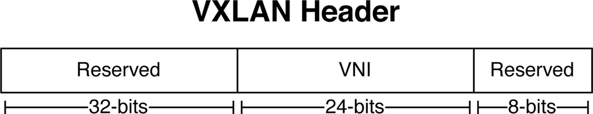
Figure 8-13. A VXLAN header
The first 32 bits of the VXLAN header are reserved. However, at least according to the IETF draft-mahalingam-dutt-dcops-vxlan, the fifth bit must have a value of 1 to indicate that it’s a valid VXLAN header. Otherwise the other 31 bits have a value of 0.
The next 24 bits are the VNI. The VNI identifies the scope of the inner MAC frame that was originated by a VM. For example, you may create multiple VNIs with overlapping MAC addresses. To recap, you can think of a VNI as a bridge domain or VLAN. The good news is that we have twice the bits to play with when compared to traditional VXLANs. VLANs can support up to 212 bridge domains. VXLAN tunnels can support up to 224 or over 16 million bridge domains. Of course, this is the theoretical limit; real-world scaling numbers are dependent on the hardware and software used.
However, simply calculating the additional overhead of 64 bits for the VXLAN header doesn’t tell the entire story when creating overlay tunnels across the network. Recall that you also need to transport this new VXLAN header across a Layer 3 network. A new outer Ethernet header, outer IP header, and outer UDP datagram is required to transport the VXLAN header across a Layer 3 network, as depicted in Figure 8-14.
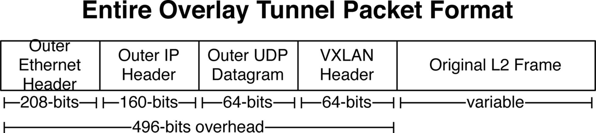
Figure 8-14. The entire overlay tunnel packet format
To sum up, an additional 496 bits of overhead is required to support a VXLAN tunnel between two VTEPs over a Layer 3 network. The total amount will vary slightly depending on the size of the original Layer 2 frame from the VM or physical server that’s being encapsulated.
NOTE
Because overlay networking requires additional overhead in a Layer 3 network, it’s a great idea to enable jumbo frames throughout the entire network. Juniper QFX5100 switches support a Maximum Transmission Unit (MTU) of up to 9,216 bytes.
Overlay Controller
When using a unicast control plane protocol such as EVPN or OVSDB, a centralized overlay controller is required. At a high level, the overlay controller performs ingress replication for MAC learning when using a unicast control plane protocol. For example, with EVPN the overlay controller would speak MP-BGP to each VTEP as well as provide BGP route reflection services to all of the other VTEPs to propagate new MAC addresses throughout the data center.
A controller is also required to provision VTEP across hypervisors and network switches. For example, every time a new hypervisor is added to the data center, it would require a management connection to the overlay controller. As new virtual networks are created, the overlay controller can create the appropriate VTEPs in the hypervisor and propagate MAC addresses.
The exception is using EVPN in a network-based VXLAN fabric, which does not require a centralized controller. Each switch will be running MP-BGP with family EVPN for MAC address learning. It’s just like building an MPLS network, but the data plane encapsulation is VXLAN. The other note is that the VXLAN VNI is globally significant as opposed to MPLS labels which are locally significant.
Virtual Routers
Up to this point in the chapter, I have only covered switching and forwarding of Ethernet frames within the same bridge domain. If a VM needs to route to another VM in a different VNI, there needs to be a Layer 3 gateway address that the VM can use as a default router. Each VNI has a virtual router (vRouter) associated with it that VMs can use as a default gateway. The vRouter is depicted as “L3 GW” in Figure 8-15.
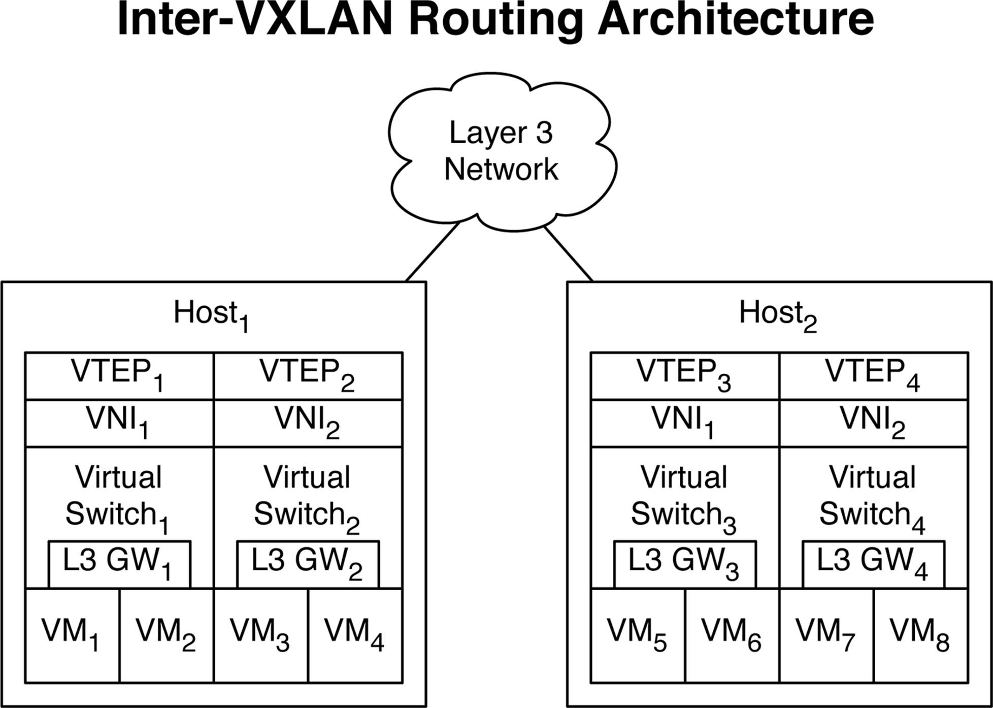
Figure 8-15. Inter-VXLAN routing architecture
Routing VM traffic
Let’s study a simple example of VM1 routing to VM3. In this scenario, the VMs are in different VNI segments and require routing. We’ll also make the assumption that VM1 and VM3 are in different networks, so that the operating system in VM1 sees that the network address of VM3 isn’t part of the same subnet and must use the default gateway. VM1 sends traffic to L3 GW1; because the L3 GW1 has full visibility of the VTEP lookup table, it sees that the destination MAC address of VM3 is associated with VTEP2. Because VM1 and VM3 are within the same host, there’s no need to encapsulate the packet. The L3 GW1 can simply locally route the traffic directly to VM3.
The next example is if VM1 needs to route traffic to VM8. The same initial steps take place. VM1 uses its default gateway of L3 GW1. The L3 GW1 receives the traffic and because it has full visibility into the VTEP tables, it sees that the destination IP address is owned by VTEP4. The L3 GW1 sends the traffic to VTEP1 which encapsulates the packet and sends it off to VTEP4. When the packet arrives at VTEP4, it strips the packet of the VXLAN encapsulation and sees that the destination address is associated with a MAC address in Virtual Switch4. The frame is forwarded through Virtual Switch4 with a source MAC address of the L3 GW4 and a destination MAC address of VM8.
Routing physical traffic
Routing VM traffic between VNIs is fairly straightforward; it all happens in software with vRouters. The more difficult use case is routing physical servers in an overlay architecture. At a high level, there are two options:
Software-Based VXLAN Routing
The physical server uses a default gateway that’s located within a VM. This means that traffic from the physical server destined to the virtual default gateway must pass through overlay tunnels until it reaches the Service VM that owns the default gateway for that VNI. When the traffic reaches the Service VM, the same process applies as if it were a VM. The major drawback is that it creates asymmetric traffic flows for physical servers.
Hardware-Based VXLAN Routing
Routing between VXLAN VNIs can happen in the networking hardware if the underlying equipment supports it. For example, the Juniper EX9200 and Juniper MX series routers support VXLAN routing. You simply create bridge domains and associate them with VNIs. Each bridge domain has a routed interface that is associated with an Integrated Routing and Bridging (IRB) interface that’s able to route traffic between bridge domains. Because the VXLAN traffic is routed in hardware, there is no performance loss and servers can transmit at line rate. Routing VXLAN traffic in the networking hardware also eliminates the asymmetric traffic patterns that exist in the software-based VXLAN routing solution, because the default gateways exist a single hop away in hardware. Also keep your eyes out for some new high-density Juniper QFX switches based on Juniper silicon that will support hardware.
The most preferable option would be to have a completely virtualized environment and not have to worry about routing physical traffic across an overlay architecture. The second best option would be to simply use the underlying networking equipment to route between VXLAN segments so that the virtual and physical servers operate in a seamless overlay architecture.
Storage
Many people assume that the storage must also take part in the overlay architecture because all of the VMs and physical servers require VTEPs to communicate with one another. However this is a common misconception. Making the assumption that the storage is IP-based, such as iSCSI or NFS, hypervisors and physical servers can simply use the underlying IP Fabric to reach the storage device directly over IP, as is demonstrated in Figure 8-16.
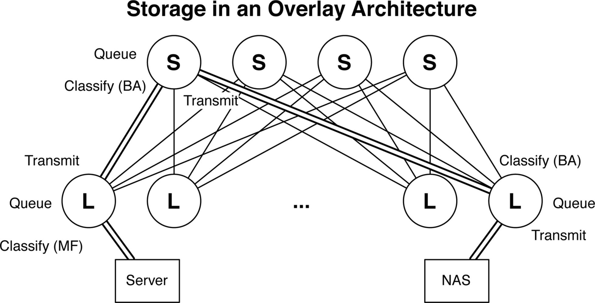
Figure 8-16. Storage in an overlay architecture
One of the benefits of using IP-based storage in an IP Fabric is that it’s reachable from any location by using Layer 3. The server in Figure 8-16 needs to access the network-attached storage (NAS) and simply routes the traffic. Although the underlying network is an IP Fabric, you can still configure lossless Ethernet queues so that storage traffic is prioritized through the network, as shown in Figure 8-16. The path between the server and NAS device is shown in a double-line in Figure 8-16. Here is what happens at each step along the way:
§ The server transmits a packet destined to the NAS device.
§ The first leaf switch receives the traffic and classifies the storage traffic by using a multifield classifier with a firewall filter.
§ The leaf switch gives priority to the storage traffic and sends the traffic to the spine switch by using a high-priority IEEE 802.1p bit.
§ The spine switch receives the traffic and identifies the high-priority storage traffic based on the IEEE 802.1p bit by using a behavior aggregate (BA).
§ The spine switch gives priority to the storage traffic and sends the traffic to the destination spine switch by using a high-priority IEEE 802.1p bit.
§ The destination leaf switch identifies the storage traffic with a BA, gives it priority, and transmits it to its final destination.
If your server and storage device support Priority-Based Flow Control (PFC)/IEEE 802.1Qbb, the Juniper QFX5100 series supports PFC over Layer 3, as well. The caveat is that PFC must operate over the IEEE 802.1p bits, therefore the point-to-point links between the spine and leaves must support IEEE 802.1Q. The result is that with lossless Ethernet queuing and PFC, servers and storage will always have guaranteed bandwidth and flow control in an overlay architecture based on an IP Fabric.
Juniper Architectures for Overlay Networks
Now that you have a better understanding of what problems an overlay architecture solves and how overlay networks operate, the next question is how can the Juniper QFX5100 family add additional value to an overlay network? Juniper QFX5100 switches support two key architectures to enable overlay architectures: Virtual Chassis Fabric (VCF) and an IP Fabric. Each architecture has its advantages and disadvantages. Most enterprise customers lean toward VCF because of its plug-and-play nature and because it’s easy to manage. Large enterprises and service providers prefer to use an IP Fabric because it offers much larger scale and a seamless routing protocol with their existing environments.
We discussed VCF in detail in Chapter 5. The power of VCF increases when you combine it with an overlay networking architecture. The first thing to recall about VCF is that the routing engine is centralized and all of the other switches in the fabric are line cards. When you create a VTEP in a VCF, you do so in the configuration only once. However, the VTEP is programmed into every single switch in the VCF, saving you from having to configure numerous times throughout your network, as shown in Figure 8-17.

Figure 8-17. VCF architecture with overlay integration
It’s also common that hypervisor hosts have multiple connections into the network. A common standard is to use 4 10GbE or 8 10GbE ports from the host into the network depending on the VM density of the host. Because VCF natively supports IEEE 802.3ad/LACP across multiple access switches, the host hypervisor can use standard LACP across all its uplinks into the network.
The really cool thing is that if there’s a physical network that needs to be integrated into the overlay architecture and requires multihoming via IEEE 802.3ad/LACP, VCF can support it and also handle the VTEP and MAC learning across LACP on behalf of the server.
Of course, VCF supports ISSU. When you need to perform network maintenance and upgrade the software, you can do so without interrupting the traffic flow of the servers.
In brief, VCF is a great solution for enterprise customers looking to move toward an overlay architecture. It offers a single point of management, so the entire data center looks like a single logical switch. Physical servers can seamlessly be integrated into the overlay architecture and support multihoming.
Configuration
Let’s jump right into the configuration details of overlay networking. There are many moving parts, as discussed in the architecture section. Let’s take each component, one by one, and see how it works on the command line.
The assumption made in this configuration exercise is that we’re integrating the Juniper QFX5100 switch into an existing VMware NSX environment running the OVSDB protocol.
Supported Hardware
First things first: let’s review which Juniper hardware supports overlay networking with built-in VTEPs into the hardware. As of this writing, there are three platforms that support hardware accelerated VTEPs:
§ Juniper QFX5100 series
§ Juniper EX9200 series
§ Juniper MX series
The Juniper QFX5100 family uses the Broadcom Trident II chipset and accommodates basic Layer 2–only VTEPs. Keep in mind that these VTEPs can only map the MAC addresses to an interface and aren’t capable of VXLAN routing. The Juniper EX9200 and MX Series are based on purpose-built Juniper silicon and support mapping of MAC addresses, interfaces, and IP addresses, allowing you to both switch and route VXLAN traffic.
Controller
Let’s make the assumption that you’re configuring a controller-based overlay network architecture by using the OVSDB control plane protocol. The first step is to configure the controller’s IP address:
[edit]
root# set protocols ovsdb controller 192.168.61.112
After you commit the configuration, the next step is to check the connection to the controller and see if it established an active connection:
dhanks@QFX5100> show ovsdb controller
VTEP controller information:
Controller IP address: 192.168.61.112
Controller protocol: ssl
Controller port: 6632
Controller connection: up
Controller seconds-since-connect: 56376
Controller seconds-since-disconnect: 0
Controller connection status: active
You can see that the connection to the VMware NSX controller is up and active.
Interfaces
The next step is to identify which interfaces are to be controlled by the OVSDB protocol. These are typically interfaces handling physical servers so that they can participate in the overlay architecture with the other VMs:
[edit]
root# set protocols ovsdb interfaces xe-0/0/3.0
Now, verify that the interface is managed by OVSDB:
dhanks@QFX5100> show ovsdb statistics interface
Interface Name: xe-0/0/3.0
Num of rx pkts: 0 Num of tx pkts: 0
Num of rx bytes: 0 Num of tx bytes: 0
Although there’s no traffic flowing through the interface yet, you can see that the interface now appears in the show ovsdb statistics command.
Switch Options
The last step is to configure the switch at a global level to be managed by OVSDB. You also need to configure the source address to be used by the switch when talking to the OVSDB controller:
[edit]
root# set switch-options ovsdb-managed
[edit]
root# set switch-options vtep-source-interface lo0.0
With the basics configured, let’s move on to the verification.
Logical Switch
Because you set a global knob called ovsdb-managed, the VMware NSX controller is able to dynamically create logical switches on the Juniper QFX5100 switch. Take a look at the logical switches on the switch:
dhanks@QFX5100> show ovsdb logical-switch
Logical switch information:
Logical Switch Name: 4918d9c6-0ac2-444f-b819-d763d577b099
Flags: Created by both
VNI: 100
Num of Remote MAC: 5
Num of Local MAC: 0
Notice the dynamically created logical switch name that ensures uniqueness across the network. This particular logical switch is associated with VNI and has already learned five remote MAC addresses.
Remote MACs
To view what MAC addresses were learned by the controller, use the following command:
dhanks@QFX5100> show ovsdb mac remote
Logical Switch Name: 4918d9c6-0ac2-444f-b819-d763d577b099
Mac IP Encapsulation Vtep
Address Address Address
40:b4:f0:07:97:f0 0.0.0.0 Vxlan over Ipv4 100.100.120.120
64:87:88:ac:42:0d 0.0.0.0 Vxlan over Ipv4 100.100.120.120
64:87:88:ac:42:18 0.0.0.0 Vxlan over Ipv4 100.100.130.130
a8:d0:e5:5b:5f:08 0.0.0.0 Vxlan over Ipv4 100.100.130.130
ff:ff:ff:ff:ff:ff 0.0.0.0 Vxlan over Ipv4 100.100.100.1
You can see that five MAC addresses have been learned. Recall that the Juniper QFX5100 series is based on the Broadcom Trident II chipset and is unable to see the IP address, because the VTEP table only holds the MAC address and interface.
OVSDB Interfaces
You can also verify that the OVSDB-managed interfaces are associated to the correct bridge domains by using the following command:
root@QFX5100> show ovsdb interface
Interface VLAN ID Bridge-domain
xe-0/0/3.0 0 4918d9c6-0ac2-444f-b819-d763d577b099
You can see that the xe-0/0/3.0 interface is correctly associated with the dynamically created bridge domain from the VMware NSX controller.
VTEPs
One of the more interesting commands that you can use is to discover what other VTEPs exist in the network. Recall that we learned five MAC addresses from the VMware NSX controller. Let’s take a look and see how many MAC addresses are associated with remote VTEPs:
dhanks@QFX5100> show ovsdb virtual-tunnel-end-point
Encapsulation Ip Address Num of MAC's
VXLAN over IPv4 100.100.100.1 1
VXLAN over IPv4 100.100.120.120 2
VXLAN over IPv4 100.100.130.130 2
You can see that a single MAC address came from the VTEP 100.100.100.1, whereas you received two MAC addresses from the VTEPs 100.100.120.120 and 100.100.130.130.
Switching Table
The last step is to see the Ethernet switching table. We can verify the MAC addresses and see which logical interface to which they’re being forwarded:
dhanks@QFX5100> show ethernet-switching table
MAC flags (S - static MAC, D - dynamic MAC, L - locally learned, P - Persistent static
SE - statistics enabled, NM - non configured MAC, R - remote PE MAC)
Ethernet switching table : 4 entries, 0 learned
Routing instance : default-switch
Vlan MAC MAC Age Logical
name address flags interface
4918d9c6-0ac2-444f-b819-d763d577b099 40:b4:f0:07:97:f0 SO - vtep.32769
4918d9c6-0ac2-444f-b819-d763d577b099 64:87:88:ac:42:0d SO - vtep.32769
4918d9c6-0ac2-444f-b819-d763d577b099 64:87:88:ac:42:18 SO - vtep.32770
4918d9c6-0ac2-444f-b819-d763d577b099 a8:d0:e5:5b:5f:08 SO - vtep.32770
Each of the five MAC addresses are being forwarded within the same bridge domain, but to different VTEPs, as shown in the Logical interface column.
Multicast VTEP Exercise
Now that you have an idea how to handle a controller-based overlay configuration, let’s move to a controller-less architecture using multicast. In this exercise, you’ll set up the topology in Figure 8-18.
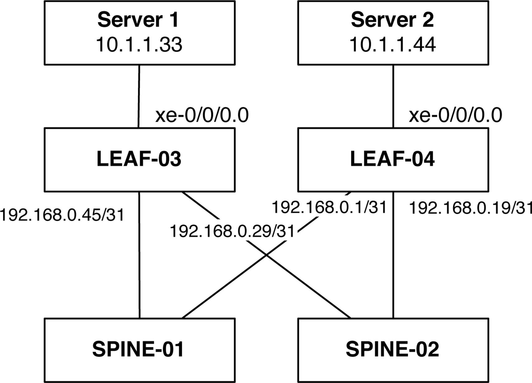
Figure 8-18. The multicast VTEP topology
The assumption is that there is a pure Layer 3 network with multicast enabled to which LEAF-03 and LEAF-04 are connected. The trick is to make Server 1 and Server 2 talk to each other over Layer 2 through a VXLAN tunnel that traverses the Layer 3 network. If Server 1 can ping Server 2 through a VXLAN tunnel, the test will be considered successful.
LEAF-03 Configuration
The first step is to configure the server-facing interface on LEAF-01 as an access port in the foobar VLAN and configure a loopback address for the switch:
interfaces {
xe-0/0/0 {
unit 0 {
family ethernet-switching {
interface-mode access;
vlan {
members foobar;
}
}
}
}
lo0 {
unit 0 {
family inet {
address 10.0.0.7/32;
}
}
}
Next, configure a static VTEP and use the loopback address as its source address:
switch-options {
vtep-source-interface lo0.0;
}
Finally, define the foobar VLAN and set up the VXLAN VNI:
vlans {
foobar {
vlan-id 100;
vxlan {
vni 100;
multicast-group 225.10.10.10;
}
}
}
Notice that we have the ability to perform VLAN normalization. As long as the VNI stays the same between remote VTEPs, the VLAN handoff can be any value back to the server. Because we’re using multicast for the MAC learning, we need to associate the VNI with a multicast group.
LEAF-04
The configuration for LEAF-04 is identical to that of LEAF-03:
interfaces {
xe-0/0/0 {
unit 0 {
family ethernet-switching {
interface-mode access;
vlan {
members foobar;
}
}
}
}
lo0 {
unit 0 {
family inet {
address 10.0.0.5/32;
}
}
}
switch-options {
vtep-source-interface lo0.0;
}
vlans {
foobar {
vlan-id 100;
vxlan {
vni 100;
multicast-group 225.10.10.10;
}
}
}
Verification
Take a moment to use some show commands to verify that you configured the basics correctly:
{master:0}
dhanks@temp-leaf-03> show vlans
Routing instance VLAN name Tag Interfaces
default-switch foobar 100
vtep.32769*
xe-0/0/0.0*
The VLAN is there and associated with the correct interface. You can also see that the VTEP is successfully created and associated with the foobar VLAN, as well.
Now, double-check your VTEP and ensure that it’s associated with the correct VLAN and multicast group:
{master:0}
dhanks@temp-leaf-03> show ethernet-switching vxlan-tunnel-end-point source
Logical System Name Id SVTEP-IP IFL L3-Idx
<default> 0 10.0.0.7 lo0.0 0
L2-RTT Bridge Domain VNID MC-Group-IP
default-switch foobar+100 100 225.10.10.10
Very cool! You see that your foobar bridge domain is bound to the VNI 100 with the correct multicast group. You can also see that your source VTEP is configured with the local loopback address of 10.0.0.7.
Take a look at what remote VTEPs have been identified:
{master:0}
root@temp-leaf-03> show ethernet-switching vxlan-tunnel-end-point remote
Logical System Name Id SVTEP-IP IFL L3-Idx
<default> 0 10.0.0.7 lo0.0 0
RVTEP-IP IFL-Idx NH-Id
10.0.0.5 567 1757
VNID MC-Group-IP
100 225.10.10.10
This is great. You can see the remote VTEP on LEAF-04 as 10.0.0.5.
Now, check the Ethernet switching table and see if the two servers have exchanged MAC addresses yet:
{master:0}
dhanks@temp-leaf-03> show ethernet-switching table
MAC flags (S - static MAC, D - dynamic MAC, L - locally learned, P - Persistent
static
SE - statistics enabled, NM - non configured MAC, R - remote PE MAC)
Ethernet switching table : 2 entries, 2 learned
Routing instance : default-switch
Vlan MAC MAC Age Logical
name address flags interface
foobar f4:b5:2f:40:66:f8 D - xe-0/0/0.0
foobar f4:b5:2f:40:66:f9 D - vtep.32769
Excellent! There is a local (f4:b5:2f:40:66:f8) and remote (f4:b5:2f:40:66:f9) MAC address in the switching table!
The last step is to ping from Server 1 to Server 2. Given that the VTEPs have discovered each other and the servers have already exchanged MAC addresses, you can be pretty confident that the ping should work:
bash# ping –c 10.1.1.44
PING 10.1.1.44 (10.1.1.44): 56 data bytes
64 bytes from 10.1.1.44: icmp_seq=0 ttl=64 time=1.127 ms
64 bytes from 10.1.1.44: icmp_seq=1 ttl=64 time=1.062 ms
64 bytes from 10.1.1.44: icmp_seq=2 ttl=64 time=1.035 ms
64 bytes from 10.1.1.44: icmp_seq=3 ttl=64 time=1.040 ms
64 bytes from 10.1.1.44: icmp_seq=4 ttl=64 time=1.064 ms
--- 10.1.1.44 ping statistics ---
5 packets transmitted, 5 packets received, 0% packet loss
round-trip min/avg/max/stddev = 1.035/1.066/1.127/0.033 ms
Indeed. Just as expected. With the tunnel successfully created, bound to the correct VLAN, and the MAC addresses showing up in the switching table, the ping has worked successfully. Server 1 is able to ping Server 2 across the same Layer 2 network through a VXLAN tunnel that’s traversing a Layer 3 network. The VTEPs on the switches are using multicast for MAC address learning, which simulates a physical Layer 2 switch characteristics to flood, filter, and forward broadcast and unknown unicast Ethernet traffic.
Summary
This chapter thoroughly discussed overlay networking in the data center. There are two categories of overlay architectures: controller-based and controller-less. The controller-based architectures use control plane–based protocols such as OVSDB (VMware NSX) and EVPN (Juniper Contrail) for MAC address learning. The controller-less options include multicast for data plane learning and MP-BGP with EVPN.
We reviewed the Juniper products that support overlay architectures and how they vary. The Juniper QFX5100 series, which is based on the Broadcom Trident II chipset, only supports Layer 2 VTEPs. The Juniper EX9200 and MX Series, which are based on the Juniper Trio chipset, offer both Layer 2 and Layer 3 VTEPs with which you can switch and route overlay traffic.
We walked through two configuration examples of overlay architectures. The first was an assumption of an IP Fabric with VMware NSX that uses the OVSDB protocol. We configured the controller, VTEP, interfaces, and walked through the commands to verify the setup. The final exercise was using a controller-less architecture that used multicast for MAC learning between the statically defined VTEPs. We were able to ping between two servers across a Layer 2 VXLAN tunnel across a Layer 3 IP Fabric.
All materials on the site are licensed Creative Commons Attribution-Sharealike 3.0 Unported CC BY-SA 3.0 & GNU Free Documentation License (GFDL)
If you are the copyright holder of any material contained on our site and intend to remove it, please contact our site administrator for approval.
© 2016-2026 All site design rights belong to S.Y.A.