Hadoop: The Definitive Guide (2015)

Part IV. Related Projects

Chapter 17. Hive

In “Information Platforms and the Rise of the Data Scientist,”^[106^] Jeff Hammerbacher describes Information Platforms as “the locus of their organization’s efforts to ingest, process, and generate information,” and how they “serve to accelerate the process of learning from empirical data.”

One of the biggest ingredients in the Information Platform built by Jeff’s team at Facebook was Apache Hive, a framework for data warehousing on top of Hadoop. Hive grew from a need to manage and learn from the huge volumes of data that Facebook was producing every day from its burgeoning social network. After trying a few different systems, the team chose Hadoop for storage and processing, since it was cost effective and met the scalability requirements.

Hive was created to make it possible for analysts with strong SQL skills (but meager Java programming skills) to run queries on the huge volumes of data that Facebook stored in HDFS. Today, Hive is a successful Apache project used by many organizations as a general-purpose, scalable data processing platform.

Of course, SQL isn’t ideal for every big data problem — it’s not a good fit for building complex machine-learning algorithms, for example — but it’s great for many analyses, and it has the huge advantage of being very well known in the industry. What’s more, SQL is the lingua franca in business intelligence tools (ODBC is a common bridge, for example), so Hive is well placed to integrate with these products.

This chapter is an introduction to using Hive. It assumes that you have working knowledge of SQL and general database architecture; as we go through Hive’s features, we’ll often compare them to the equivalent in a traditional RDBMS.

Installing Hive

In normal use, Hive runs on your workstation and converts your SQL query into a series of jobs for execution on a Hadoop cluster. Hive organizes data into tables, which provide a means for attaching structure to data stored in HDFS. Metadata — such as table schemas — is stored in a database called the metastore.

When starting out with Hive, it is convenient to run the metastore on your local machine. In this configuration, which is the default, the Hive table definitions that you create will be local to your machine, so you can’t share them with other users. We’ll see how to configure a shared remote metastore, which is the norm in production environments, in The Metastore.

Installation of Hive is straightforward. As a prerequisite, you need to have the same version of Hadoop installed locally that your cluster is running.^[107^] Of course, you may choose to run Hadoop locally, either in standalone or pseudodistributed mode, while getting started with Hive. These options are all covered in Appendix A.

WHICH VERSIONS OF HADOOP DOES HIVE WORK WITH?

Any given release of Hive is designed to work with multiple versions of Hadoop. Generally, Hive works with the latest stable release of Hadoop, as well as supporting a number of older versions, listed in the release notes. You don’t need to do anything special to tell Hive which version of Hadoop you are using, beyond making sure that the hadoop executable is on the path or setting the HADOOP_HOME environment variable.

Download a release, and unpack the tarball in a suitable place on your workstation:

% tar xzf apache-hive-x.y.z-bin.tar.gz

It’s handy to put Hive on your path to make it easy to launch:

% export HIVE_HOME=~/sw/apache-hive-x.y.z-bin

% export PATH=$PATH:$HIVE_HOME/bin

Now type hive to launch the Hive shell:

% hive

hive>

The Hive Shell

The shell is the primary way that we will interact with Hive, by issuing commands in HiveQL. HiveQL is Hive’s query language, a dialect of SQL. It is heavily influenced by MySQL, so if you are familiar with MySQL, you should feel at home using Hive.

When starting Hive for the first time, we can check that it is working by listing its tables — there should be none. The command must be terminated with a semicolon to tell Hive to execute it:

hive> SHOW TABLES;

OK

Time taken: 0.473 seconds

Like SQL, HiveQL is generally case insensitive (except for string comparisons), so show tables; works equally well here. The Tab key will autocomplete Hive keywords and functions.

For a fresh install, the command takes a few seconds to run as it lazily creates the metastore database on your machine. (The database stores its files in a directory called metastore_db, which is relative to the location from which you ran the hive command.)

You can also run the Hive shell in noninteractive mode. The -f option runs the commands in the specified file, which is script.q in this example:

% hive -f script.q

For short scripts, you can use the -e option to specify the commands inline, in which case the final semicolon is not required:

% hive -e 'SELECT * FROM dummy'

OK

X

Time taken: 1.22 seconds, Fetched: 1 row(s)

NOTE

It’s useful to have a small table of data to test queries against, such as trying out functions in SELECT expressions using literal data (see Operators and Functions). Here’s one way of populating a single-row table:

% echo 'X' > /tmp/dummy.txt

% hive -e "CREATE TABLE dummy (value STRING); \

LOAD DATA LOCAL INPATH '/tmp/dummy.txt' \

OVERWRITE INTO TABLE dummy"

In both interactive and noninteractive mode, Hive will print information to standard error — such as the time taken to run a query — during the course of operation. You can suppress these messages using the -S option at launch time, which has the effect of showing only the output result for queries:

% hive -S -e 'SELECT * FROM dummy'

X

Other useful Hive shell features include the ability to run commands on the host operating system by using a ! prefix to the command and the ability to access Hadoop filesystems using the dfs command.

An Example

Let’s see how to use Hive to run a query on the weather dataset we explored in earlier chapters. The first step is to load the data into Hive’s managed storage. Here we’ll have Hive use the local filesystem for storage; later we’ll see how to store tables in HDFS.

Just like an RDBMS, Hive organizes its data into tables. We create a table to hold the weather data using the CREATE TABLE statement:

CREATE TABLE records (year STRING, temperature INT, quality INT)

ROW FORMAT DELIMITED

FIELDS TERMINATED BY '\t';

The first line declares a records table with three columns: year, temperature, and quality. The type of each column must be specified, too. Here the year is a string, while the other two columns are integers.

So far, the SQL is familiar. The ROW FORMAT clause, however, is particular to HiveQL. This declaration is saying that each row in the data file is tab-delimited text. Hive expects there to be three fields in each row, corresponding to the table columns, with fields separated by tabs and rows by newlines.

Next, we can populate Hive with the data. This is just a small sample, for exploratory purposes:

LOAD DATA LOCAL INPATH 'input/ncdc/micro-tab/sample.txt'

OVERWRITE INTO TABLE records;

Running this command tells Hive to put the specified local file in its warehouse directory. This is a simple filesystem operation. There is no attempt, for example, to parse the file and store it in an internal database format, because Hive does not mandate any particular file format. Files are stored verbatim; they are not modified by Hive.

In this example, we are storing Hive tables on the local filesystem (fs.defaultFS is set to its default value of file:///). Tables are stored as directories under Hive’s warehouse directory, which is controlled by the hive.metastore.warehouse.dir property and defaults to/user/hive/warehouse.

Thus, the files for the records table are found in the /user/hive/warehouse/records directory on the local filesystem:

% ls /user/hive/warehouse/records/

sample.txt

In this case, there is only one file, sample.txt, but in general there can be more, and Hive will read all of them when querying the table.

The OVERWRITE keyword in the LOAD DATA statement tells Hive to delete any existing files in the directory for the table. If it is omitted, the new files are simply added to the table’s directory (unless they have the same names, in which case they replace the old files).

Now that the data is in Hive, we can run a query against it:

hive> SELECT year, MAX(temperature)

> FROM records

> WHERE temperature != 9999 AND quality IN (0, 1, 4, 5, 9)

> GROUP BY year;

1949 111

1950 22

This SQL query is unremarkable. It is a SELECT statement with a GROUP BY clause for grouping rows into years, which uses the MAX aggregate function to find the maximum temperature for each year group. The remarkable thing is that Hive transforms this query into a job, which it executes on our behalf, then prints the results to the console. There are some nuances, such as the SQL constructs that Hive supports and the format of the data that we can query — and we explore some of these in this chapter — but it is the ability to execute SQL queries against our raw data that gives Hive its power.

Running Hive

In this section, we look at some more practical aspects of running Hive, including how to set up Hive to run against a Hadoop cluster and a shared metastore. In doing so, we’ll see Hive’s architecture in some detail.

Configuring Hive

Hive is configured using an XML configuration file like Hadoop’s. The file is called hive-site.xml and is located in Hive’s conf directory. This file is where you can set properties that you want to set every time you run Hive. The same directory contains hive-default.xml, which documents the properties that Hive exposes and their default values.

You can override the configuration directory that Hive looks for in hive-site.xml by passing the --config option to the hive command:

% hive --config /Users/tom/dev/hive-conf

Note that this option specifies the containing directory, not hive-site.xml itself. It can be useful when you have multiple site files — for different clusters, say — that you switch between on a regular basis. Alternatively, you can set the HIVE_CONF_DIR environment variable to the configuration directory for the same effect.

The hive-site.xml file is a natural place to put the cluster connection details: you can specify the filesystem and resource manager using the usual Hadoop properties, fs.defaultFS and yarn.resourcemanager.address (see Appendix A for more details on configuring Hadoop). If not set, they default to the local filesystem and the local (in-process) job runner — just like they do in Hadoop — which is very handy when trying out Hive on small trial datasets. Metastore configuration settings (covered in The Metastore) are commonly found in hive-site.xml, too.

Hive also permits you to set properties on a per-session basis, by passing the -hiveconf option to the hive command. For example, the following command sets the cluster (in this case, to a pseudodistributed cluster) for the duration of the session:

% hive -hiveconf fs.defaultFS=hdfs://localhost \

-hiveconf mapreduce.framework.name=yarn \

-hiveconf yarn.resourcemanager.address=localhost:8032

WARNING

If you plan to have more than one Hive user sharing a Hadoop cluster, you need to make the directories that Hive uses writable by all users. The following commands will create the directories and set their permissions appropriately:

% hadoop fs -mkdir /tmp

% hadoop fs -chmod a+w /tmp

% hadoop fs -mkdir -p /user/hive/warehouse

% hadoop fs -chmod a+w /user/hive/warehouse

If all users are in the same group, then permissions g+w are sufficient on the warehouse directory.

You can change settings from within a session, too, using the SET command. This is useful for changing Hive settings for a particular query. For example, the following command ensures buckets are populated according to the table definition (see Buckets):

hive> SET hive.enforce.bucketing=true;

To see the current value of any property, use SET with just the property name:

hive> SET hive.enforce.bucketing;

hive.enforce.bucketing=true

By itself, SET will list all the properties (and their values) set by Hive. Note that the list will not include Hadoop defaults, unless they have been explicitly overridden in one of the ways covered in this section. Use SET -v to list all the properties in the system, including Hadoop defaults.

There is a precedence hierarchy to setting properties. In the following list, lower numbers take precedence over higher numbers:

1. The Hive SET command

2. The command-line -hiveconf option

3. hive-site.xml and the Hadoop site files (core-site.xml, hdfs-site.xml, mapred-site.xml, and yarn-site.xml)

4. The Hive defaults and the Hadoop default files (core-default.xml, hdfs-default.xml, mapred-default.xml, and yarn-default.xml)

Setting configuration properties for Hadoop is covered in more detail in Which Properties Can I Set?.

Execution engines

Hive was originally written to use MapReduce as its execution engine, and that is still the default. It is now also possible to run Hive using Apache Tez as its execution engine, and work is underway to support Spark (see Chapter 19), too. Both Tez and Spark are general directed acyclic graph (DAG) engines that offer more flexibility and higher performance than MapReduce. For example, unlike MapReduce, where intermediate job output is materialized to HDFS, Tez and Spark can avoid replication overhead by writing the intermediate output to local disk, or even store it in memory (at the request of the Hive planner).

The execution engine is controlled by the hive.execution.engine property, which defaults to mr (for MapReduce). It’s easy to switch the execution engine on a per-query basis, so you can see the effect of a different engine on a particular query. Set Hive to use Tez as follows:

hive> SET hive.execution.engine=tez;

Note that Tez needs to be installed on the Hadoop cluster first; see the Hive documentation for up-to-date details on how to do this.

Logging

You can find Hive’s error log on the local filesystem at ${java.io.tmpdir}/${user.name}/hive.log. It can be very useful when trying to diagnose configuration problems or other types of error. Hadoop’s MapReduce task logs are also a useful resource for troubleshooting; see Hadoop Logs for where to find them.

On many systems, ${java.io.tmpdir} is /tmp, but if it’s not, or if you want to set the logging directory to be another location, then use the following:

% hive -hiveconf hive.log.dir='/tmp/${user.name}'

The logging configuration is in conf/hive-log4j.properties, and you can edit this file to change log levels and other logging-related settings. However, often it’s more convenient to set logging configuration for the session. For example, the following handy invocation will send debug messages to the console:

% hive -hiveconf hive.root.logger=DEBUG,console

Hive Services

The Hive shell is only one of several services that you can run using the hive command. You can specify the service to run using the --service option. Type hive --service help to get a list of available service names; some of the most useful ones are described in the following list:

cli

The command-line interface to Hive (the shell). This is the default service.

hiveserver2

Runs Hive as a server exposing a Thrift service, enabling access from a range of clients written in different languages. HiveServer 2 improves on the original HiveServer by supporting authentication and multiuser concurrency. Applications using the Thrift, JDBC, and ODBC connectors need to run a Hive server to communicate with Hive. Set the hive.server2.thrift.port configuration property to specify the port the server will listen on (defaults to 10000).

beeline

A command-line interface to Hive that works in embedded mode (like the regular CLI), or by connecting to a HiveServer 2 process using JDBC.

hwi

The Hive Web Interface. A simple web interface that can be used as an alternative to the CLI without having to install any client software. See also Hue for a more fully featured Hadoop web interface that includes applications for running Hive queries and browsing the Hive metastore.

jar

The Hive equivalent of hadoop jar, a convenient way to run Java applications that includes both Hadoop and Hive classes on the classpath.

metastore

By default, the metastore is run in the same process as the Hive service. Using this service, it is possible to run the metastore as a standalone (remote) process. Set the METASTORE_PORT environment variable (or use the -p command-line option) to specify the port the server will listen on (defaults to 9083).

Hive clients

If you run Hive as a server (hive --service hiveserver2), there are a number of different mechanisms for connecting to it from applications (the relationship between Hive clients and Hive services is illustrated in Figure 17-1):

Thrift Client

The Hive server is exposed as a Thrift service, so it’s possible to interact with it using any programming language that supports Thrift. There are third-party projects providing clients for Python and Ruby; for more details, see the Hive wiki.

JDBC driver

Hive provides a Type 4 (pure Java) JDBC driver, defined in the class org.apache.hadoop.hive.jdbc.HiveDriver. When configured with a JDBC URI of the form jdbc:hive2://host:port/dbname, a Java application will connect to a Hive server running in a separate process at the given host and port. (The driver makes calls to an interface implemented by the Hive Thrift Client using the Java Thrift bindings.)

You may alternatively choose to connect to Hive via JDBC in embedded mode using the URI jdbc:hive2://. In this mode, Hive runs in the same JVM as the application invoking it; there is no need to launch it as a standalone server, since it does not use the Thrift service or the Hive Thrift Client.

The Beeline CLI uses the JDBC driver to communicate with Hive.

ODBC driver

An ODBC driver allows applications that support the ODBC protocol (such as business intelligence software) to connect to Hive. The Apache Hive distribution does not ship with an ODBC driver, but several vendors make one freely available. (Like the JDBC driver, ODBC drivers use Thrift to communicate with the Hive server.)

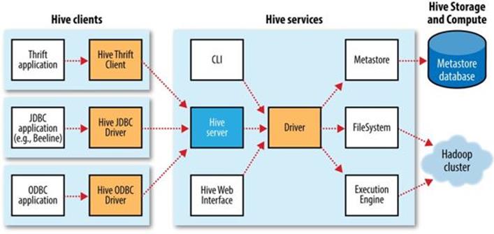
Figure 17-1. Hive architecture

The Metastore

The metastore is the central repository of Hive metadata. The metastore is divided into two pieces: a service and the backing store for the data. By default, the metastore service runs in the same JVM as the Hive service and contains an embedded Derby database instance backed by the local disk. This is called the embedded metastore configuration (see Figure 17-2).

Using an embedded metastore is a simple way to get started with Hive; however, only one embedded Derby database can access the database files on disk at any one time, which means you can have only one Hive session open at a time that accesses the same metastore. Trying to start a second session produces an error when it attempts to open a connection to the metastore.

The solution to supporting multiple sessions (and therefore multiple users) is to use a standalone database. This configuration is referred to as a local metastore, since the metastore service still runs in the same process as the Hive service but connects to a database running in a separate process, either on the same machine or on a remote machine. Any JDBC-compliant database may be used by setting the javax.jdo.option.* configuration properties listed in Table 17-1.^[108^]

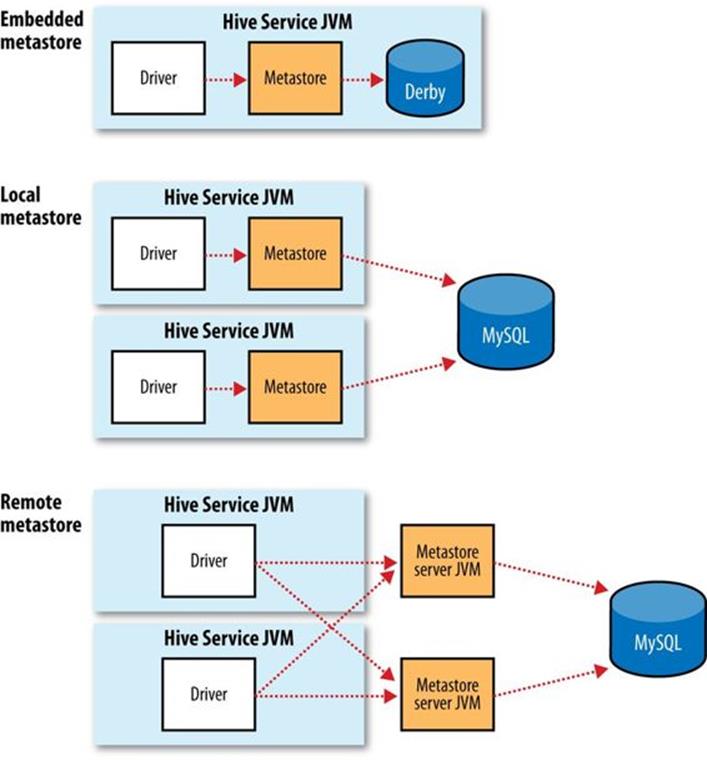
Figure 17-2. Metastore configurations

MySQL is a popular choice for the standalone metastore. In this case, the javax.jdo.option.ConnectionURL property is set to jdbc:mysql://host/dbname?createDatabaseIfNotExist=true, and javax.jdo.option.ConnectionDriverName is set to com.mysql.jdbc.Driver. (The username and password should be set too, of course.) The JDBC driver JAR file for MySQL (Connector/J) must be on Hive’s classpath, which is simply achieved by placing it in Hive’s lib directory.

Going a step further, there’s another metastore configuration called a remote metastore, where one or more metastore servers run in separate processes to the Hive service. This brings better manageability and security because the database tier can be completely firewalled off, and the clients no longer need the database credentials.

A Hive service is configured to use a remote metastore by setting hive.metastore.uris to the metastore server URI(s), separated by commas if there is more than one. Metastore server URIs are of the form thrift://host:port, where the port corresponds to the one set byMETASTORE_PORT when starting the metastore server (see Hive Services).

Table 17-1. Important metastore configuration properties

Comparison with Traditional Databases

Although Hive resembles a traditional database in many ways (such as supporting a SQL interface), its original HDFS and MapReduce underpinnings mean that there are a number of architectural differences that have directly influenced the features that Hive supports. Over time, however, these limitations have been (and continue to be) removed, with the result that Hive looks and feels more like a traditional database with every year that passes.

Schema on Read Versus Schema on Write

In a traditional database, a table’s schema is enforced at data load time. If the data being loaded doesn’t conform to the schema, then it is rejected. This design is sometimes called schema on write because the data is checked against the schema when it is written into the database.

Hive, on the other hand, doesn’t verify the data when it is loaded, but rather when a query is issued. This is called schema on read.

There are trade-offs between the two approaches. Schema on read makes for a very fast initial load, since the data does not have to be read, parsed, and serialized to disk in the database’s internal format. The load operation is just a file copy or move. It is more flexible, too: consider having two schemas for the same underlying data, depending on the analysis being performed. (This is possible in Hive using external tables; see Managed Tables and External Tables.)

Schema on write makes query time performance faster because the database can index columns and perform compression on the data. The trade-off, however, is that it takes longer to load data into the database. Furthermore, there are many scenarios where the schema is not known at load time, so there are no indexes to apply, because the queries have not been formulated yet. These scenarios are where Hive shines.

Updates, Transactions, and Indexes

Updates, transactions, and indexes are mainstays of traditional databases. Yet, until recently, these features have not been considered a part of Hive’s feature set. This is because Hive was built to operate over HDFS data using MapReduce, where full-table scans are the norm and a table update is achieved by transforming the data into a new table. For a data warehousing application that runs over large portions of the dataset, this works well.

Hive has long supported adding new rows in bulk to an existing table by using INSERT INTO to add new data files to a table. From release 0.14.0, finer-grained changes are possible, so you can call INSERT INTO TABLE...VALUES to insert small batches of values computed in SQL. In addition, it is possible to UPDATE and DELETE rows in a table.

HDFS does not provide in-place file updates, so changes resulting from inserts, updates, and deletes are stored in small delta files. Delta files are periodically merged into the base table files by MapReduce jobs that are run in the background by the metastore. These features only work in the context of transactions (introduced in Hive 0.13.0), so the table they are being used on needs to have transactions enabled on it. Queries reading the table are guaranteed to see a consistent snapshot of the table.

Hive also has support for table- and partition-level locking. Locks prevent, for example, one process from dropping a table while another is reading from it. Locks are managed transparently using ZooKeeper, so the user doesn’t have to acquire or release them, although it is possible to get information about which locks are being held via the SHOW LOCKS statement. By default, locks are not enabled.

Hive indexes can speed up queries in certain cases. A query such as SELECT * from t WHERE x = a, for example, can take advantage of an index on column x, since only a small portion of the table’s files need to be scanned. There are currently two index types: compact and bitmap. (The index implementation was designed to be pluggable, so it’s expected that a variety of implementations will emerge for different use cases.)

Compact indexes store the HDFS block numbers of each value, rather than each file offset, so they don’t take up much disk space but are still effective for the case where values are clustered together in nearby rows. Bitmap indexes use compressed bitsets to efficiently store the rows that a particular value appears in, and they are usually appropriate for low-cardinality columns (such as gender or country).

SQL-on-Hadoop Alternatives

In the years since Hive was created, many other SQL-on-Hadoop engines have emerged to address some of Hive’s limitations. Cloudera Impala, an open source interactive SQL engine, was one of the first, giving an order of magnitude performance boost compared to Hive running on MapReduce. Impala uses a dedicated daemon that runs on each datanode in the cluster. When a client runs a query it contacts an arbitrary node running an Impala daemon, which acts as a coordinator node for the query. The coordinator sends work to other Impala daemons in the cluster and combines their results into the full result set for the query. Impala uses the Hive metastore and supports Hive formats and most HiveQL constructs (plus SQL-92), so in practice it is straightforward to migrate between the two systems, or to run both on the same cluster.

Hive has not stood still, though, and since Impala was launched, the “Stinger” initiative by Hortonworks has improved the performance of Hive through support for Tez as an execution engine, and the addition of a vectorized query engine among other improvements.

Other prominent open source Hive alternatives include Presto from Facebook, Apache Drill, and Spark SQL. Presto and Drill have similar architectures to Impala, although Drill targets SQL:2011 rather than HiveQL. Spark SQL uses Spark as its underlying engine, and lets you embed SQL queries in Spark programs.

NOTE

Spark SQL is different to using the Spark execution engine from within Hive (“Hive on Spark,” see Execution engines). Hive, on Spark provides all the features of Hive since it is a part of the Hive project. Spark SQL, on the other hand, is a new SQL engine that offers some level of Hive compatibility.

Apache Phoenix takes a different approach entirely: it provides SQL on HBase. SQL access is through a JDBC driver that turns queries into HBase scans and takes advantage of HBase coprocessors to perform server-side aggregation. Metadata is stored in HBase, too.

HiveQL

Hive’s SQL dialect, called HiveQL, is a mixture of SQL-92, MySQL, and Oracle’s SQL dialect. The level of SQL-92 support has improved over time, and will likely continue to get better. HiveQL also provides features from later SQL standards, such as window functions (also known as analytic functions) from SQL:2003. Some of Hive’s non-standard extensions to SQL were inspired by MapReduce, such as multitable inserts (see Multitable insert) and the TRANSFORM, MAP, and REDUCE clauses (see MapReduce Scripts).

This chapter does not provide a complete reference to HiveQL; for that, see the Hive documentation. Instead, we focus on commonly used features and pay particular attention to features that diverge from either SQL-92 or popular databases such as MySQL. Table 17-2 provides a high-level comparison of SQL and HiveQL.

Table 17-2. A high-level comparison of SQL and HiveQL

Data Types

Hive supports both primitive and complex data types. Primitives include numeric, Boolean, string, and timestamp types. The complex data types include arrays, maps, and structs. Hive’s data types are listed in Table 17-3. Note that the literals shown are those used from within HiveQL; they are not the serialized forms used in the table’s storage format (see Storage Formats).

Table 17-3. Hive data types

Primitive types

Hive’s primitive types correspond roughly to Java’s, although some names are influenced by MySQL’s type names (some of which, in turn, overlap with SQL-92’s). There is a BOOLEAN type for storing true and false values. There are four signed integral types: TINYINT, SMALLINT, INT, and BIGINT, which are equivalent to Java’s byte, short, int, and long primitive types, respectively (they are 1-byte, 2-byte, 4-byte, and 8-byte signed integers).

Hive’s floating-point types, FLOAT and DOUBLE, correspond to Java’s float and double, which are 32-bit and 64-bit floating-point numbers.

The DECIMAL data type is used to represent arbitrary-precision decimals, like Java’s BigDecimal, and are commonly used for representing currency values. DECIMAL values are stored as unscaled integers. The precision is the number of digits in the unscaled value, and the scale is the number of digits to the right of the decimal point. So, for example, DECIMAL(5,2) stores numbers between −999.99 and 999.99. If the scale is omitted then it defaults to 0, so DECIMAL(5)stores numbers in the range −99,999 to 99,999 (i.e., integers). If the precision is omitted then it defaults to 10, so DECIMAL is equivalent to DECIMAL(10,0). The maximum allowed precision is 38, and the scale must be no larger than the precision.

There are three Hive data types for storing text. STRING is a variable-length character string with no declared maximum length. (The theoretical maximum size STRING that may be stored is 2 GB, although in practice it may be inefficient to materialize such large values. Sqoop has large object support; see Importing Large Objects.) VARCHAR types are similar except they are declared with a maximum length between 1 and 65355; for example, VARCHAR(100). CHAR types are fixed-length strings that are padded with trailing spaces if necessary; for example, CHAR(100). Trailing spaces are ignored for the purposes of string comparison of CHAR values.

The BINARY data type is for storing variable-length binary data.

The TIMESTAMP data type stores timestamps with nanosecond precision. Hive comes with UDFs for converting between Hive timestamps, Unix timestamps (seconds since the Unix epoch), and strings, which makes most common date operations tractable. TIMESTAMP does not encapsulate a time zone; however, the to_utc_timestamp and from_utc_timestamp functions make it possible to do time zone conversions.

The DATE data type stores a date with year, month, and day components.

Complex types

Hive has four complex types: ARRAY, MAP, STRUCT, and UNION. ARRAY and MAP are like their namesakes in Java, whereas a STRUCT is a record type that encapsulates a set of named fields. A UNION specifies a choice of data types; values must match exactly one of these types.

Complex types permit an arbitrary level of nesting. Complex type declarations must specify the type of the fields in the collection, using an angled bracket notation, as illustrated in this table definition with three columns (one for each complex type):

CREATE TABLE complex (

c1 ARRAY<INT>,

c2 MAP<STRING, INT>,

c3 STRUCT<a:STRING, b:INT, c:DOUBLE>,

c4 UNIONTYPE<STRING, INT>

);

If we load the table with one row of data for ARRAY, MAP, STRUCT, and UNION, as shown in the “Literal examples” column in Table 17-3 (we’ll see the file format needed to do this in Storage Formats), the following query demonstrates the field accessor operators for each type:

hive> SELECT c1[0], c2['b'], c3.c, c4 FROM complex;

1 2 1.0 {1:63}

Operators and Functions

The usual set of SQL operators is provided by Hive: relational operators (such as x = 'a' for testing equality, x IS NULL for testing nullity, and x LIKE 'a%' for pattern matching), arithmetic operators (such as x + 1 for addition), and logical operators (such as x OR y for logical OR). The operators match those in MySQL, which deviates from SQL-92 because || is logical OR, not string concatenation. Use the concat function for the latter in both MySQL and Hive.

Hive comes with a large number of built-in functions — too many to list here — divided into categories that include mathematical and statistical functions, string functions, date functions (for operating on string representations of dates), conditional functions, aggregate functions, and functions for working with XML (using the xpath function) and JSON.

You can retrieve a list of functions from the Hive shell by typing SHOW FUNCTIONS.^[109^] To get brief usage instructions for a particular function, use the DESCRIBE command:

hive> DESCRIBE FUNCTION length;

length(str | binary) - Returns the length of str or number of bytes in binary

data

In the case when there is no built-in function that does what you want, you can write your own; see User-Defined Functions.

Conversions

Primitive types form a hierarchy that dictates the implicit type conversions Hive will perform in function and operator expressions. For example, a TINYINT will be converted to an INT if an expression expects an INT; however, the reverse conversion will not occur, and Hive will return an error unless the CAST operator is used.

The implicit conversion rules can be summarized as follows. Any numeric type can be implicitly converted to a wider type, or to a text type (STRING, VARCHAR, CHAR). All the text types can be implicitly converted to another text type. Perhaps surprisingly, they can also be converted toDOUBLE or DECIMAL. BOOLEAN types cannot be converted to any other type, and they cannot be implicitly converted to any other type in expressions. TIMESTAMP and DATE can be implicitly converted to a text type.

You can perform explicit type conversion using CAST. For example, CAST('1' AS INT) will convert the string '1' to the integer value 1. If the cast fails — as it does in CAST('X' AS INT), for example — the expression returns NULL.

Tables

A Hive table is logically made up of the data being stored and the associated metadata describing the layout of the data in the table. The data typically resides in HDFS, although it may reside in any Hadoop filesystem, including the local filesystem or S3. Hive stores the metadata in arelational database and not in, say, HDFS (see The Metastore).

In this section, we look in more detail at how to create tables, the different physical storage formats that Hive offers, and how to import data into tables.

MULTIPLE DATABASE/SCHEMA SUPPORT

Many relational databases have a facility for multiple namespaces, which allows users and applications to be segregated into different databases or schemas. Hive supports the same facility and provides commands such as CREATE DATABASE dbname, USE dbname, and DROP DATABASE dbname. You can fully qualify a table by writing dbname.tablename. If no database is specified, tables belong to the default database.

Managed Tables and External Tables

When you create a table in Hive, by default Hive will manage the data, which means that Hive moves the data into its warehouse directory. Alternatively, you may create an external table, which tells Hive to refer to the data that is at an existing location outside the warehouse directory.

The difference between the two table types is seen in the LOAD and DROP semantics. Let’s consider a managed table first.

When you load data into a managed table, it is moved into Hive’s warehouse directory. For example, this:

CREATE TABLE managed_table (dummy STRING);

LOAD DATA INPATH '/user/tom/data.txt' INTO table managed_table;

will move the file hdfs://user/tom/data.txt into Hive’s warehouse directory for the managed_table table, which is hdfs://user/hive/warehouse/managed_table.^[110^]

NOTE

The load operation is very fast because it is just a move or rename within a filesystem. However, bear in mind that Hive does not check that the files in the table directory conform to the schema declared for the table, even for managed tables. If there is a mismatch, this will become apparent at query time, often by the query returning NULL for a missing field. You can check that the data is being parsed correctly by issuing a simple SELECT statement to retrieve a few rows directly from the table.

If the table is later dropped, using:

DROP TABLE managed_table;

the table, including its metadata and its data, is deleted. It bears repeating that since the initial LOAD performed a move operation, and the DROP performed a delete operation, the data no longer exists anywhere. This is what it means for Hive to manage the data.

An external table behaves differently. You control the creation and deletion of the data. The location of the external data is specified at table creation time:

CREATE EXTERNAL TABLE external_table (dummy STRING)

LOCATION '/user/tom/external_table';

LOAD DATA INPATH '/user/tom/data.txt' INTO TABLE external_table;

With the EXTERNAL keyword, Hive knows that it is not managing the data, so it doesn’t move it to its warehouse directory. Indeed, it doesn’t even check whether the external location exists at the time it is defined. This is a useful feature because it means you can create the data lazily after creating the table.

When you drop an external table, Hive will leave the data untouched and only delete the metadata.

So how do you choose which type of table to use? In most cases, there is not much difference between the two (except of course for the difference in DROP semantics), so it is a just a matter of preference. As a rule of thumb, if you are doing all your processing with Hive, then use managed tables, but if you wish to use Hive and other tools on the same dataset, then use external tables. A common pattern is to use an external table to access an initial dataset stored in HDFS (created by another process), then use a Hive transform to move the data into a managed Hive table. This works the other way around, too; an external table (not necessarily on HDFS) can be used to export data from Hive for other applications to use.^[111^]

Another reason for using external tables is when you wish to associate multiple schemas with the same dataset.

Partitions and Buckets

Hive organizes tables into partitions — a way of dividing a table into coarse-grained parts based on the value of a partition column, such as a date. Using partitions can make it faster to do queries on slices of the data.

Tables or partitions may be subdivided further into buckets to give extra structure to the data that may be used for more efficient queries. For example, bucketing by user ID means we can quickly evaluate a user-based query by running it on a randomized sample of the total set of users.

Partitions

To take an example where partitions are commonly used, imagine logfiles where each record includes a timestamp. If we partition by date, then records for the same date will be stored in the same partition. The advantage to this scheme is that queries that are restricted to a particular date or set of dates can run much more efficiently, because they only need to scan the files in the partitions that the query pertains to. Notice that partitioning doesn’t preclude more wide-ranging queries: it is still feasible to query the entire dataset across many partitions.

A table may be partitioned in multiple dimensions. For example, in addition to partitioning logs by date, we might also subpartition each date partition by country to permit efficient queries by location.

Partitions are defined at table creation time using the PARTITIONED BY clause,^[112^] which takes a list of column definitions. For the hypothetical logfiles example, we might define a table with records comprising a timestamp and the log line itself:

CREATE TABLE logs (ts BIGINT, line STRING)

PARTITIONED BY (dt STRING, country STRING);

When we load data into a partitioned table, the partition values are specified explicitly:

LOAD DATA LOCAL INPATH 'input/hive/partitions/file1'

INTO TABLE logs

PARTITION (dt='2001-01-01', country='GB');

At the filesystem level, partitions are simply nested subdirectories of the table directory. After loading a few more files into the logs table, the directory structure might look like this:

/user/hive/warehouse/logs

├── dt=2001-01-01/

│ ├── country=GB/

│ │ ├── file1

│ │ └── file2

│ └── country=US/

│ └── file3

└── dt=2001-01-02/

├── country=GB/

│ └── file4

└── country=US/

├── file5

└── file6

The logs table has two date partitions (2001-01-01 and 2001-01-02, corresponding to subdirectories called dt=2001-01-01 and dt=2001-01-02); and two country subpartitions (GB and US, corresponding to nested subdirectories called country=GB and country=US). The datafiles reside in the leaf directories.

We can ask Hive for the partitions in a table using SHOW PARTITIONS:

hive> SHOW PARTITIONS logs;

dt=2001-01-01/country=GB

dt=2001-01-01/country=US

dt=2001-01-02/country=GB

dt=2001-01-02/country=US

One thing to bear in mind is that the column definitions in the PARTITIONED BY clause are full-fledged table columns, called partition columns; however, the datafiles do not contain values for these columns, since they are derived from the directory names.

You can use partition columns in SELECT statements in the usual way. Hive performs input pruning to scan only the relevant partitions. For example:

SELECT ts, dt, line

FROM logs

WHERE country='GB';

will only scan file1, file2, and file4. Notice, too, that the query returns the values of the dt partition column, which Hive reads from the directory names since they are not in the datafiles.

Buckets

There are two reasons why you might want to organize your tables (or partitions) into buckets. The first is to enable more efficient queries. Bucketing imposes extra structure on the table, which Hive can take advantage of when performing certain queries. In particular, a join of two tables that are bucketed on the same columns — which include the join columns — can be efficiently implemented as a map-side join.

The second reason to bucket a table is to make sampling more efficient. When working with large datasets, it is very convenient to try out queries on a fraction of your dataset while you are in the process of developing or refining them. We will see how to do efficient sampling at the end of this section.

First, let’s see how to tell Hive that a table should be bucketed. We use the CLUSTERED BY clause to specify the columns to bucket on and the number of buckets:

CREATE TABLE bucketed_users (id INT, name STRING)

CLUSTERED BY (id) INTO 4 BUCKETS;

Here we are using the user ID to determine the bucket (which Hive does by hashing the value and reducing modulo the number of buckets), so any particular bucket will effectively have a random set of users in it.

In the map-side join case, where the two tables are bucketed in the same way, a mapper processing a bucket of the left table knows that the matching rows in the right table are in its corresponding bucket, so it need only retrieve that bucket (which is a small fraction of all the data stored in the right table) to effect the join. This optimization also works when the number of buckets in the two tables are multiples of each other; they do not have to have exactly the same number of buckets. The HiveQL for joining two bucketed tables is shown in Map joins.

The data within a bucket may additionally be sorted by one or more columns. This allows even more efficient map-side joins, since the join of each bucket becomes an efficient merge sort. The syntax for declaring that a table has sorted buckets is:

CREATE TABLE bucketed_users (id INT, name STRING)

CLUSTERED BY (id) SORTED BY (id ASC) INTO 4 BUCKETS;

How can we make sure the data in our table is bucketed? Although it’s possible to load data generated outside Hive into a bucketed table, it’s often easier to get Hive to do the bucketing, usually from an existing table.

WARNING

Hive does not check that the buckets in the datafiles on disk are consistent with the buckets in the table definition (either in number or on the basis of bucketing columns). If there is a mismatch, you may get an error or undefined behavior at query time. For this reason, it is advisable to get Hive to perform the bucketing.

Take an unbucketed users table:

hive> SELECT * FROM users;

0 Nat

2 Joe

3 Kay

4 Ann

To populate the bucketed table, we need to set the hive.enforce.bucketing property to true so that Hive knows to create the number of buckets declared in the table definition. Then it is just a matter of using the INSERT command:

INSERT OVERWRITE TABLE bucketed_users

SELECT * FROM users;

Physically, each bucket is just a file in the table (or partition) directory. The filename is not important, but bucket n is the nth file when arranged in lexicographic order. In fact, buckets correspond to MapReduce output file partitions: a job will produce as many buckets (output files) as reduce tasks. We can see this by looking at the layout of the bucketed_users table we just created. Running this command:

hive> dfs -ls /user/hive/warehouse/bucketed_users;

shows that four files were created, with the following names (the names are generated by Hive):

000000_0

000001_0

000002_0

000003_0

The first bucket contains the users with IDs 0 and 4, since for an INT the hash is the integer itself, and the value is reduced modulo the number of buckets — four, in this case:^[113^]

hive> dfs -cat /user/hive/warehouse/bucketed_users/000000_0;

0Nat

4Ann

We can see the same thing by sampling the table using the TABLESAMPLE clause, which restricts the query to a fraction of the buckets in the table rather than the whole table:

hive> SELECT * FROM bucketed_users

> TABLESAMPLE(BUCKET 1 OUT OF 4 ON id);

4 Ann

0 Nat

Bucket numbering is 1-based, so this query retrieves all the users from the first of four buckets. For a large, evenly distributed dataset, approximately one-quarter of the table’s rows would be returned. It’s possible to sample a number of buckets by specifying a different proportion (which need not be an exact multiple of the number of buckets, as sampling is not intended to be a precise operation). For example, this query returns half of the buckets:

hive> SELECT * FROM bucketed_users

> TABLESAMPLE(BUCKET 1 OUT OF 2 ON id);

4 Ann

0 Nat

2 Joe

Sampling a bucketed table is very efficient because the query only has to read the buckets that match the TABLESAMPLE clause. Contrast this with sampling a nonbucketed table using the rand() function, where the whole input dataset is scanned, even if only a very small sample isneeded:

hive> SELECT * FROM users

> TABLESAMPLE(BUCKET 1 OUT OF 4 ON rand());

2 Joe

Storage Formats

There are two dimensions that govern table storage in Hive: the row format and the file format. The row format dictates how rows, and the fields in a particular row, are stored. In Hive parlance, the row format is defined by a SerDe, a portmanteau word for a Serializer-Deserializer.

When acting as a deserializer, which is the case when querying a table, a SerDe will deserialize a row of data from the bytes in the file to objects used internally by Hive to operate on that row of data. When used as a serializer, which is the case when performing an INSERT or CTAS (see Importing Data), the table’s SerDe will serialize Hive’s internal representation of a row of data into the bytes that are written to the output file.

The file format dictates the container format for fields in a row. The simplest format is a plain-text file, but there are row-oriented and column-oriented binary formats available, too.

The default storage format: Delimited text

When you create a table with no ROW FORMAT or STORED AS clauses, the default format is delimited text with one row per line.^[114^]

The default row delimiter is not a tab character, but the Ctrl-A character from the set of ASCII control codes (it has ASCII code 1). The choice of Ctrl-A, sometimes written as ^A in documentation, came about because it is less likely to be a part of the field text than a tab character. There is no means for escaping delimiter characters in Hive, so it is important to choose ones that don’t occur in data fields.

The default collection item delimiter is a Ctrl-B character, used to delimit items in an ARRAY or STRUCT, or in key-value pairs in a MAP. The default map key delimiter is a Ctrl-C character, used to delimit the key and value in a MAP. Rows in a table are delimited by a newline character.

WARNING

The preceding description of delimiters is correct for the usual case of flat data structures, where the complex types contain only primitive types. For nested types, however, this isn’t the whole story, and in fact the level of the nesting determines the delimiter.

For an array of arrays, for example, the delimiters for the outer array are Ctrl-B characters, as expected, but for the inner array they are Ctrl-C characters, the next delimiter in the list. If you are unsure which delimiters Hive uses for a particular nested structure, you can run a command like:

CREATE TABLE nested

AS

SELECT array(array(1, 2), array(3, 4))

FROM dummy;

and then use hexdump or something similar to examine the delimiters in the output file.

Hive actually supports eight levels of delimiters, corresponding to ASCII codes 1, 2, ... 8, but you can override only the first three.

Thus, the statement:

CREATE TABLE ...;

is identical to the more explicit:

CREATE TABLE ...

ROW FORMAT DELIMITED

FIELDS TERMINATED BY '\001'

COLLECTION ITEMS TERMINATED BY '\002'

MAP KEYS TERMINATED BY '\003'

LINES TERMINATED BY '\n'

STORED AS TEXTFILE;

Notice that the octal form of the delimiter characters can be used — 001 for Ctrl-A, for instance.

Internally, Hive uses a SerDe called LazySimpleSerDe for this delimited format, along with the line-oriented MapReduce text input and output formats we saw in Chapter 8. The “lazy” prefix comes about because it deserializes fields lazily — only as they are accessed. However, it is not a compact format because fields are stored in a verbose textual format, so a Boolean value, for instance, is written as the literal string true or false.

The simplicity of the format has a lot going for it, such as making it easy to process with other tools, including MapReduce programs or Streaming, but there are more compact and performant binary storage formats that you might consider using. These are discussed next.

Binary storage formats: Sequence files, Avro datafiles, Parquet files, RCFiles, and ORCFiles

Using a binary format is as simple as changing the STORED AS clause in the CREATE TABLE statement. In this case, the ROW FORMAT is not specified, since the format is controlled by the underlying binary file format.

Binary formats can be divided into two categories: row-oriented formats and column-oriented formats. Generally speaking, column-oriented formats work well when queries access only a small number of columns in the table, whereas row-oriented formats are appropriate when a large number of columns of a single row are needed for processing at the same time.

The two row-oriented formats supported natively in Hive are Avro datafiles (see Chapter 12) and sequence files (see SequenceFile). Both are general-purpose, splittable, compressible formats; in addition, Avro supports schema evolution and multiple language bindings. From Hive 0.14.0, a table can be stored in Avro format using:

SET hive.exec.compress.output=true;

SET avro.output.codec=snappy;

CREATE TABLE ... STORED AS AVRO;

Notice that compression is enabled on the table by setting the relevant properties.

Similarly, the declaration STORED AS SEQUENCEFILE can be used to store sequence files in Hive. The properties for compression are listed in Using Compression in MapReduce.

Hive has native support for the Parquet (see Chapter 13), RCFile, and ORCFile column-oriented binary formats (see Other File Formats and Column-Oriented Formats). Here is an example of creating a copy of a table in Parquet format using CREATE TABLE...AS SELECT (see CREATE TABLE...AS SELECT):

CREATE TABLE users_parquet STORED AS PARQUET

AS

SELECT * FROM users;

Using a custom SerDe: RegexSerDe

Let’s see how to use a custom SerDe for loading data. We’ll use a contrib SerDe that uses a regular expression for reading the fixed-width station metadata from a text file:

CREATE TABLE stations (usaf STRING, wban STRING, name STRING)

ROW FORMAT SERDE 'org.apache.hadoop.hive.contrib.serde2.RegexSerDe'

WITH SERDEPROPERTIES (

"input.regex" = "(\\d{6}) (\\d{5}) (.{29}) .*"

);

In previous examples, we have used the DELIMITED keyword to refer to delimited text in the ROW FORMAT clause. In this example, we instead specify a SerDe with the SERDE keyword and the fully qualified classname of the Java class that implements the SerDe,org.apache.hadoop.hive.contrib.serde2.RegexSerDe.

SerDes can be configured with extra properties using the WITH SERDEPROPERTIES clause. Here we set the input.regex property, which is specific to RegexSerDe.

input.regex is the regular expression pattern to be used during deserialization to turn the line of text forming the row into a set of columns. Java regular expression syntax is used for the matching, and columns are formed from capturing groups of parentheses.^[115^] In this example, there are three capturing groups for usaf (a six-digit identifier), wban (a five-digit identifier), and name (a fixed-width column of 29 characters).

To populate the table, we use a LOAD DATA statement as before:

LOAD DATA LOCAL INPATH "input/ncdc/metadata/stations-fixed-width.txt"

INTO TABLE stations;

Recall that LOAD DATA copies or moves the files to Hive’s warehouse directory (in this case, it’s a copy because the source is the local filesystem). The table’s SerDe is not used for the load operation.

When we retrieve data from the table the SerDe is invoked for deserialization, as we can see from this simple query, which correctly parses the fields for each row:

hive> SELECT * FROM stations LIMIT 4;

010000 99999 BOGUS NORWAY

010003 99999 BOGUS NORWAY

010010 99999 JAN MAYEN

010013 99999 ROST

As this example demonstrates, RegexSerDe can be useful for getting data into Hive, but due to its inefficiency it should not be used for general-purpose storage. Consider copying the data into a binary storage format instead.

Storage handlers

Storage handlers are used for storage systems that Hive cannot access natively, such as HBase. Storage handlers are specified using a STORED BY clause, instead of the ROW FORMAT and STORED AS clauses. For more information on HBase integration, see the Hive wiki.

Importing Data

We’ve already seen how to use the LOAD DATA operation to import data into a Hive table (or partition) by copying or moving files to the table’s directory. You can also populate a table with data from another Hive table using an INSERT statement, or at creation time using the CTASconstruct, which is an abbreviation used to refer to CREATE TABLE...AS SELECT.

If you want to import data from a relational database directly into Hive, have a look at Sqoop; this is covered in Imported Data and Hive.

Inserts

Here’s an example of an INSERT statement:

INSERT OVERWRITE TABLE target

SELECT col1, col2

FROM source;

For partitioned tables, you can specify the partition to insert into by supplying a PARTITION clause:

INSERT OVERWRITE TABLE target

PARTITION (dt='2001-01-01')

SELECT col1, col2

FROM source;

The OVERWRITE keyword means that the contents of the target table (for the first example) or the 2001-01-01 partition (for the second example) are replaced by the results of the SELECT statement. If you want to add records to an already populated nonpartitioned table or partition, useINSERT INTO TABLE.

You can specify the partition dynamically by determining the partition value from the SELECT statement:

INSERT OVERWRITE TABLE target

PARTITION (dt)

SELECT col1, col2, dt

FROM source;

This is known as a dynamic partition insert.

NOTE

From Hive 0.14.0, you can use the INSERT INTO TABLE...VALUES statement for inserting a small collection of records specified in literal form.

Multitable insert

In HiveQL, you can turn the INSERT statement around and start with the FROM clause for the same effect:

FROM source

INSERT OVERWRITE TABLE target

SELECT col1, col2;

The reason for this syntax becomes clear when you see that it’s possible to have multiple INSERT clauses in the same query. This so-called multitable insert is more efficient than multiple INSERT statements because the source table needs to be scanned only once to produce the multiple disjoint outputs.

Here’s an example that computes various statistics over the weather dataset:

FROM records2

INSERT OVERWRITE TABLE stations_by_year

SELECT year, COUNT(DISTINCT station)

GROUP BY year

INSERT OVERWRITE TABLE records_by_year

SELECT year, COUNT(1)

GROUP BY year

INSERT OVERWRITE TABLE good_records_by_year

SELECT year, COUNT(1)

WHERE temperature != 9999 AND quality IN (0, 1, 4, 5, 9)

GROUP BY year;

There is a single source table (records2), but three tables to hold the results from three different queries over the source.

CREATE TABLE...AS SELECT

It’s often very convenient to store the output of a Hive query in a new table, perhaps because it is too large to be dumped to the console or because there are further processing steps to carry out on the result.

The new table’s column definitions are derived from the columns retrieved by the SELECT clause. In the following query, the target table has two columns named col1 and col2 whose types are the same as the ones in the source table:

CREATE TABLE target

AS

SELECT col1, col2

FROM source;

A CTAS operation is atomic, so if the SELECT query fails for some reason, the table is not created.

Altering Tables

Because Hive uses the schema-on-read approach, it’s flexible in permitting a table’s definition to change after the table has been created. The general caveat, however, is that in many cases, it is up to you to ensure that the data is changed to reflect the new structure.

You can rename a table using the ALTER TABLE statement:

ALTER TABLE source RENAME TO target;

In addition to updating the table metadata, ALTER TABLE moves the underlying table directory so that it reflects the new name. In the current example, /user/hive/warehouse/source is renamed to /user/hive/warehouse/target. (An external table’s underlying directory is not moved; only the metadata is updated.)

Hive allows you to change the definition for columns, add new columns, or even replace all existing columns in a table with a new set.

For example, consider adding a new column:

ALTER TABLE target ADD COLUMNS (col3 STRING);

The new column col3 is added after the existing (nonpartition) columns. The datafiles are not updated, so queries will return null for all values of col3 (unless of course there were extra fields already present in the files). Because Hive does not permit updating existing records, you will need to arrange for the underlying files to be updated by another mechanism. For this reason, it is more common to create a new table that defines new columns and populates them using a SELECT statement.

Changing a column’s metadata, such as a column’s name or data type, is more straightforward, assuming that the old data type can be interpreted as the new data type.

To learn more about how to alter a table’s structure, including adding and dropping partitions, changing and replacing columns, and changing table and SerDe properties, see the Hive wiki.

Dropping Tables

The DROP TABLE statement deletes the data and metadata for a table. In the case of external tables, only the metadata is deleted; the data is left untouched.

If you want to delete all the data in a table but keep the table definition, use TRUNCATE TABLE. For example:

TRUNCATE TABLE my_table;

This doesn’t work for external tables; instead, use dfs -rmr (from the Hive shell) to remove the external table directory directly.

In a similar vein, if you want to create a new, empty table with the same schema as another table, then use the LIKE keyword:

CREATE TABLE new_table LIKE existing_table;

Querying Data

This section discusses how to use various forms of the SELECT statement to retrieve data from Hive.

Sorting and Aggregating

Sorting data in Hive can be achieved by using a standard ORDER BY clause. ORDER BY performs a parallel total sort of the input (like that described in Total Sort). When a globally sorted result is not required — and in many cases it isn’t — you can use Hive’s nonstandard extension, SORT BY, instead. SORT BY produces a sorted file per reducer.

In some cases, you want to control which reducer a particular row goes to — typically so you can perform some subsequent aggregation. This is what Hive’s DISTRIBUTE BY clause does. Here’s an example to sort the weather dataset by year and temperature, in such a way as to ensure that all the rows for a given year end up in the same reducer partition:^[116^]

hive> FROM records2

> SELECT year, temperature

> DISTRIBUTE BY year

> SORT BY year ASC, temperature DESC;

1949 111

1949 78

1950 22

1950 0

1950 -11

A follow-on query (or a query that nests this query as a subquery; see Subqueries) would be able to use the fact that each year’s temperatures were grouped and sorted (in descending order) in the same file.

If the columns for SORT BY and DISTRIBUTE BY are the same, you can use CLUSTER BY as a shorthand for specifying both.

MapReduce Scripts

Using an approach like Hadoop Streaming, the TRANSFORM, MAP, and REDUCE clauses make it possible to invoke an external script or program from Hive. Suppose we want to use a script to filter out rows that don’t meet some condition, such as the script in Example 17-1, which removes poor-quality readings.

Example 17-1. Python script to filter out poor-quality weather records

#!/usr/bin/env python

import re

import sys

for line insys.stdin:

(year, temp, q) = line.strip().split()

if (temp != "9999" andre.match("[01459]", q)):

print "%s\t%s" % (year, temp)

We can use the script as follows:

hive> ADD FILE /Users/tom/book-workspace/hadoop-book/ch17-hive/

src/main/python/is_good_quality.py;

hive> FROM records2

> SELECT TRANSFORM(year, temperature, quality)

> USING 'is_good_quality.py'

> AS year, temperature;

1950 0

1950 22

1950 -11

1949 111

1949 78

Before running the query, we need to register the script with Hive. This is so Hive knows to ship the file to the Hadoop cluster (see Distributed Cache).

The query itself streams the year, temperature, and quality fields as a tab-separated line to the is_good_quality.py script, and parses the tab-separated output into year and temperature fields to form the output of the query.

This example has no reducers. If we use a nested form for the query, we can specify a map and a reduce function. This time we use the MAP and REDUCE keywords, but SELECT TRANSFORM in both cases would have the same result. (Example 2-10 includes the source for themax_temperature_reduce.py script):

FROM (

FROM records2

MAP year, temperature, quality

USING 'is_good_quality.py'

AS year, temperature) map_output

REDUCE year, temperature

USING 'max_temperature_reduce.py'

AS year, temperature;

Joins

One of the nice things about using Hive, rather than raw MapReduce, is that Hive makes performing commonly used operations very simple. Join operations are a case in point, given how involved they are to implement in MapReduce (see Joins).

Inner joins

The simplest kind of join is the inner join, where each match in the input tables results in a row in the output. Consider two small demonstration tables, sales (which lists the names of people and the IDs of the items they bought) and things (which lists the item IDs and their names):

hive> SELECT * FROM sales;

Joe 2

Hank 4

Ali 0

Eve 3

Hank 2

hive> SELECT * FROM things;

2 Tie

4 Coat

3 Hat

1 Scarf

We can perform an inner join on the two tables as follows:

hive> SELECT sales.*, things.*

> FROM sales JOIN things ON (sales.id = things.id);

Joe 2 2 Tie

Hank 4 4 Coat

Eve 3 3 Hat

Hank 2 2 Tie

The table in the FROM clause (sales) is joined with the table in the JOIN clause (things), using the predicate in the ON clause. Hive only supports equijoins, which means that only equality can be used in the join predicate, which here matches on the id column in both tables.

In Hive, you can join on multiple columns in the join predicate by specifying a series of expressions, separated by AND keywords. You can also join more than two tables by supplying additional JOIN...ON... clauses in the query. Hive is intelligent about trying to minimize the number of MapReduce jobs to perform the joins.

NOTE

Hive (like MySQL and Oracle) allows you to list the join tables in the FROM clause and specify the join condition in the WHERE clause of a SELECT statement. For example, the following is another way of expressing the query we just saw:

SELECT sales.*, things.*

FROM sales, things

WHERE sales.id = things.id;

A single join is implemented as a single MapReduce job, but multiple joins can be performed in less than one MapReduce job per join if the same column is used in the join condition.^[117^] You can see how many MapReduce jobs Hive will use for any particular query by prefixing itwith the EXPLAIN keyword:

EXPLAIN

SELECT sales.*, things.*

FROM sales JOIN things ON (sales.id = things.id);

The EXPLAIN output includes many details about the execution plan for the query, including the abstract syntax tree, the dependency graph for the stages that Hive will execute, and information about each stage. Stages may be MapReduce jobs or operations such as file moves. For even more detail, prefix the query with EXPLAIN EXTENDED.

Hive currently uses a rule-based query optimizer for determining how to execute a query, but a cost-based optimizer is available from Hive 0.14.0.

Outer joins

Outer joins allow you to find nonmatches in the tables being joined. In the current example, when we performed an inner join, the row for Ali did not appear in the output, because the ID of the item she purchased was not present in the things table. If we change the join type to LEFT OUTER JOIN, the query will return a row for every row in the left table (sales), even if there is no corresponding row in the table it is being joined to (things):

hive> SELECT sales.*, things.*

> FROM sales LEFT OUTER JOIN things ON (sales.id = things.id);

Joe 2 2 Tie

Hank 4 4 Coat

Ali 0 NULL NULL

Eve 3 3 Hat

Hank 2 2 Tie

Notice that the row for Ali is now returned, and the columns from the things table are NULL because there is no match.

Hive also supports right outer joins, which reverses the roles of the tables relative to the left join. In this case, all items from the things table are included, even those that weren’t purchased by anyone (a scarf):

hive> SELECT sales.*, things.*

> FROM sales RIGHT OUTER JOIN things ON (sales.id = things.id);

Joe 2 2 Tie

Hank 2 2 Tie

Hank 4 4 Coat

Eve 3 3 Hat

NULL NULL 1 Scarf

Finally, there is a full outer join, where the output has a row for each row from both tables in the join:

hive> SELECT sales.*, things.*

> FROM sales FULL OUTER JOIN things ON (sales.id = things.id);

Ali 0 NULL NULL

NULL NULL 1 Scarf

Hank 2 2 Tie

Joe 2 2 Tie

Eve 3 3 Hat

Hank 4 4 Coat

Semi joins

Consider this IN subquery, which finds all the items in the things table that are in the sales table:

SELECT *

FROM things

WHERE things.id IN (SELECT id from sales);

We can also express it as follows:

hive> SELECT *

> FROM things LEFT SEMI JOIN sales ON (sales.id = things.id);

2 Tie

4 Coat

3 Hat

There is a restriction that we must observe for LEFT SEMI JOIN queries: the right table (sales) may appear only in the ON clause. It cannot be referenced in a SELECT expression, for example.

Map joins

Consider the original inner join again:

SELECT sales.*, things.*

FROM sales JOIN things ON (sales.id = things.id);

If one table is small enough to fit in memory, as things is here, Hive can load it into memory to perform the join in each of the mappers. This is called a map join.

The job to execute this query has no reducers, so this query would not work for a RIGHT or FULL OUTER JOIN, since absence of matching can be detected only in an aggregating (reduce) step across all the inputs.

Map joins can take advantage of bucketed tables (see Buckets), since a mapper working on a bucket of the left table needs to load only the corresponding buckets of the right table to perform the join. The syntax for the join is the same as for the in-memory case shown earlier; however, you also need to enable the optimization with the following:

SET hive.optimize.bucketmapjoin=true;

Subqueries

A subquery is a SELECT statement that is embedded in another SQL statement. Hive has limited support for subqueries, permitting a subquery in the FROM clause of a SELECT statement, or in the WHERE clause in certain cases.

NOTE

Hive allows uncorrelated subqueries, where the subquery is a self-contained query referenced by an IN or EXISTS statement in the WHERE clause. Correlated subqueries, where the subquery references the outer query, are not currently supported.

The following query finds the mean maximum temperature for every year and weather station:

SELECT station, year, AVG(max_temperature)

FROM (

SELECT station, year, MAX(temperature) AS max_temperature

FROM records2

WHERE temperature != 9999 AND quality IN (0, 1, 4, 5, 9)

GROUP BY station, year

) mt

GROUP BY station, year;

The FROM subquery is used to find the maximum temperature for each station/date combination, and then the outer query uses the AVG aggregate function to find the average of the maximum temperature readings for each station/date combination.

The outer query accesses the results of the subquery like it does a table, which is why the subquery must be given an alias (mt). The columns of the subquery have to be given unique names so that the outer query can refer to them.

Views

A view is a sort of “virtual table” that is defined by a SELECT statement. Views can be used to present data to users in a way that differs from the way it is actually stored on disk. Often, the data from existing tables is simplified or aggregated in a particular way that makes it convenient for further processing. Views may also be used to restrict users’ access to particular subsets of tables that they are authorized to see.

In Hive, a view is not materialized to disk when it is created; rather, the view’s SELECT statement is executed when the statement that refers to the view is run. If a view performs extensive transformations on the base tables or is used frequently, you may choose to manually materialize it by creating a new table that stores the contents of the view (see CREATE TABLE...AS SELECT).

We can use views to rework the query from the previous section for finding the mean maximum temperature for every year and weather station. First, let’s create a view for valid records — that is, records that have a particular quality value:

CREATE VIEW valid_records

AS

SELECT *

FROM records2

WHERE temperature != 9999 AND quality IN (0, 1, 4, 5, 9);

When we create a view, the query is not run; it is simply stored in the metastore. Views are included in the output of the SHOW TABLES command, and you can see more details about a particular view, including the query used to define it, by issuing the DESCRIBE EXTENDED view_namecommand.

Next, let’s create a second view of maximum temperatures for each station and year. It is based on the valid_records view:

CREATE VIEW max_temperatures (station, year, max_temperature)

AS

SELECT station, year, MAX(temperature)

FROM valid_records

GROUP BY station, year;

In this view definition, we list the column names explicitly. We do this because the maximum temperature column is an aggregate expression, and otherwise Hive would create a column alias for us (such as _c2). We could equally well have used an AS clause in the SELECT to name the column.

With the views in place, we can now use them by running a query:

SELECT station, year, AVG(max_temperature)

FROM max_temperatures

GROUP BY station, year;

The result of the query is the same as that of running the one that uses a subquery. In particular, Hive creates the same number of MapReduce jobs for both: two in each case, one for each GROUP BY. This example shows that Hive can combine a query on a view into a sequence of jobs that is equivalent to writing the query without using a view. In other words, Hive won’t needlessly materialize a view, even at execution time.

Views in Hive are read-only, so there is no way to load or insert data into an underlying base table via a view.

User-Defined Functions

Sometimes the query you want to write can’t be expressed easily (or at all) using the built-in functions that Hive provides. By allowing you to write a user-defined function (UDF), Hive makes it easy to plug in your own processing code and invoke it from a Hive query.

UDFs have to be written in Java, the language that Hive itself is written in. For other languages, consider using a SELECT TRANSFORM query, which allows you to stream data through a user-defined script (MapReduce Scripts).

There are three types of UDF in Hive: (regular) UDFs, user-defined aggregate functions (UDAFs), and user-defined table-generating functions (UDTFs). They differ in the number of rows that they accept as input and produce as output:

§ A UDF operates on a single row and produces a single row as its output. Most functions, such as mathematical functions and string functions, are of this type.

§ A UDAF works on multiple input rows and creates a single output row. Aggregate functions include such functions as COUNT and MAX.

§ A UDTF operates on a single row and produces multiple rows — a table — as output.

Table-generating functions are less well known than the other two types, so let’s look at an example. Consider a table with a single column, x, which contains arrays of strings. It’s instructive to take a slight detour to see how the table is defined and populated:

CREATE TABLE arrays (x ARRAY<STRING>)

ROW FORMAT DELIMITED

FIELDS TERMINATED BY '\001'

COLLECTION ITEMS TERMINATED BY '\002';

Notice that the ROW FORMAT clause specifies that the entries in the array are delimited by Ctrl-B characters. The example file that we are going to load has the following contents, where ^B is a representation of the Ctrl-B character to make it suitable for printing:

a^Bb

c^Bd^Be

After running a LOAD DATA command, the following query confirms that the data was loaded correctly:

hive> SELECT * FROM arrays;

["a","b"]

["c","d","e"]

Next, we can use the explode UDTF to transform this table. This function emits a row for each entry in the array, so in this case the type of the output column y is STRING. The result is that the table is flattened into five rows:

hive> SELECT explode(x) AS y FROM arrays;

a

b

c

d

e

SELECT statements using UDTFs have some restrictions (e.g., they cannot retrieve additional column expressions), which make them less useful in practice. For this reason, Hive supports LATERAL VIEW queries, which are more powerful. LATERAL VIEW queries are not covered here, but you may find out more about them in the Hive wiki.

Writing a UDF

To illustrate the process of writing and using a UDF, we’ll write a simple UDF to trim characters from the ends of strings. Hive already has a built-in function called trim, so we’ll call ours strip. The code for the Strip Java class is shown in Example 17-2.

Example 17-2. A UDF for stripping characters from the ends of strings

package com.hadoopbook.hive;

import org.apache.commons.lang.StringUtils;

import org.apache.hadoop.hive.ql.exec.UDF;

import org.apache.hadoop.io.Text;

public class Strip extends UDF {

private Text result = new Text();

public Text evaluate(Text str) {

if (str == null) {

return null;

}

result.set(StringUtils.strip(str.toString()));

return result;

} public Text evaluate(Text str, String stripChars) {

if (str == null) {

return null;

}

result.set(StringUtils.strip(str.toString(), stripChars));

return result;

}

}

A UDF must satisfy the following two properties:

§ A UDF must be a subclass of org.apache.hadoop.hive.ql.exec.UDF.

§ A UDF must implement at least one evaluate() method.

The evaluate() method is not defined by an interface, since it may take an arbitrary number of arguments, of arbitrary types, and it may return a value of arbitrary type. Hive introspects the UDF to find the evaluate() method that matches the Hive function that was invoked.

The Strip class has two evaluate() methods. The first strips leading and trailing whitespace from the input, and the second can strip any of a set of supplied characters from the ends of the string. The actual string processing is delegated to the StringUtils class from the Apache Commons project, which makes the only noteworthy part of the code the use of Text from the Hadoop Writable library. Hive actually supports Java primitives in UDFs (and a few other types, such as java.util.List and java.util.Map), so a signature like:

public String evaluate(String str)

would work equally well. However, by using Text we can take advantage of object reuse, which can bring efficiency savings, so this is preferred in general.

To use the UDF in Hive, we first need to package the compiled Java class in a JAR file. You can do this by typing mvn package with the book’s example code. Next, we register the function in the metastore and give it a name using the CREATE FUNCTION statement:

CREATE FUNCTION strip AS 'com.hadoopbook.hive.Strip'

USING JAR '/path/to/hive-examples.jar';

When using Hive locally, a local file path is sufficient, but on a cluster you should copy the JAR file into HDFS and use an HDFS URI in the USING JAR clause.

The UDF is now ready to be used, just like a built-in function:

hive> SELECT strip(' bee ') FROM dummy;

bee

hive> SELECT strip('banana', 'ab') FROM dummy;

nan

Notice that the UDF’s name is not case sensitive:

hive> SELECT STRIP(' bee ') FROM dummy;

bee

If you want to remove the function, use the DROP FUNCTION statement:

DROP FUNCTION strip;

It’s also possible to create a function for the duration of the Hive session, so it is not persisted in the metastore, using the TEMPORARY keyword:

ADD JAR /path/to/hive-examples.jar;

CREATE TEMPORARY FUNCTION strip AS 'com.hadoopbook.hive.Strip';

When using temporary functions, it may be useful to create a .hiverc file in your home directory containing the commands to define your UDFs. The file will be automatically run at the beginning of each Hive session.

NOTE

As an alternative to calling ADD JAR at launch time, you can specify a path where Hive looks for auxiliary JAR files to put on its classpath (including the task classpath). This technique is useful for automatically adding your own library of UDFs every time you run Hive.

There are two ways of specifying the path. Either pass the --auxpath option to the hive command:

% hive --auxpath /path/to/hive-examples.jar

or set the HIVE_AUX_JARS_PATH environment variable before invoking Hive. The auxiliary path may be a comma-separated list of JAR file paths or a directory containing JAR files.

Writing a UDAF

An aggregate function is more difficult to write than a regular UDF. Values are aggregated in chunks (potentially across many tasks), so the implementation has to be capable of combining partial aggregations into a final result. The code to achieve this is best explained by example, so let’s look at the implementation of a simple UDAF for calculating the maximum of a collection of integers (Example 17-3).

Example 17-3. A UDAF for calculating the maximum of a collection of integers

package com.hadoopbook.hive;

import org.apache.hadoop.hive.ql.exec.UDAF;

import org.apache.hadoop.hive.ql.exec.UDAFEvaluator;

import org.apache.hadoop.io.IntWritable;

public class Maximum extends UDAF {

public static class MaximumIntUDAFEvaluator implements UDAFEvaluator {

private IntWritable result;

public void init() {

result = null;

}

public boolean iterate(IntWritable value) {

if (value == null) {

return true;

}

if (result == null) {

result = new IntWritable(value.get());

} else {

result.set(Math.max(result.get(), value.get()));

}

return true;

}

public IntWritable terminatePartial() {

return result;

}

public boolean merge(IntWritable other) {

return iterate(other);

}

public IntWritable terminate() {

return result;

}

}

}

The class structure is slightly different from the one for UDFs. A UDAF must be a subclass of org.apache.hadoop.hive.ql.exec.UDAF (note the “A” in UDAF) and contain one or more nested static classes implementing org.apache.hadoop.hive.ql.exec.UDAFEvaluator. In this example, there is a single nested class, MaximumIntUDAFEvaluator, but we could add more evaluators, such as MaximumLongUDAFEvaluator, MaximumFloatUDAFEvaluator, and so on, to provide overloaded forms of the UDAF for finding the maximum of a collection of longs, floats, and so on.

An evaluator must implement five methods, described in turn here (the flow is illustrated in Figure 17-3):

init()

The init() method initializes the evaluator and resets its internal state. In MaximumIntUDAFEvaluator, we set the IntWritable object holding the final result to null. We use null to indicate that no values have been aggregated yet, which has the desirable effect of making the maximum value of an empty set NULL.

iterate()

The iterate() method is called every time there is a new value to be aggregated. The evaluator should update its internal state with the result of performing the aggregation. The arguments that iterate() takes correspond to those in the Hive function from which it was called. In this example, there is only one argument. The value is first checked to see whether it is null, and if it is, it is ignored. Otherwise, the result instance variable is set either to value’s integer value (if this is the first value that has been seen) or to the larger of the current result andvalue (if one or more values have already been seen). We return true to indicate that the input value was valid.

terminatePartial()

The terminatePartial() method is called when Hive wants a result for the partial aggregation. The method must return an object that encapsulates the state of the aggregation. In this case, an IntWritable suffices because it encapsulates either the maximum value seen or null if no values have been processed.

merge()

The merge() method is called when Hive decides to combine one partial aggregation with another. The method takes a single object, whose type must correspond to the return type of the terminatePartial() method. In this example, the merge() method can simply delegate to theiterate() method because the partial aggregation is represented in the same way as a value being aggregated. This is not generally the case (we’ll see a more general example later), and the method should implement the logic to combine the evaluator’s state with the state of the partial aggregation.

terminate()

The terminate() method is called when the final result of the aggregation is needed. The evaluator should return its state as a value. In this case, we return the result instance variable.

Let’s exercise our new function:

hive> CREATE TEMPORARY FUNCTION maximum AS 'com.hadoopbook.hive.Maximum';

hive> SELECT maximum(temperature) FROM records;

111

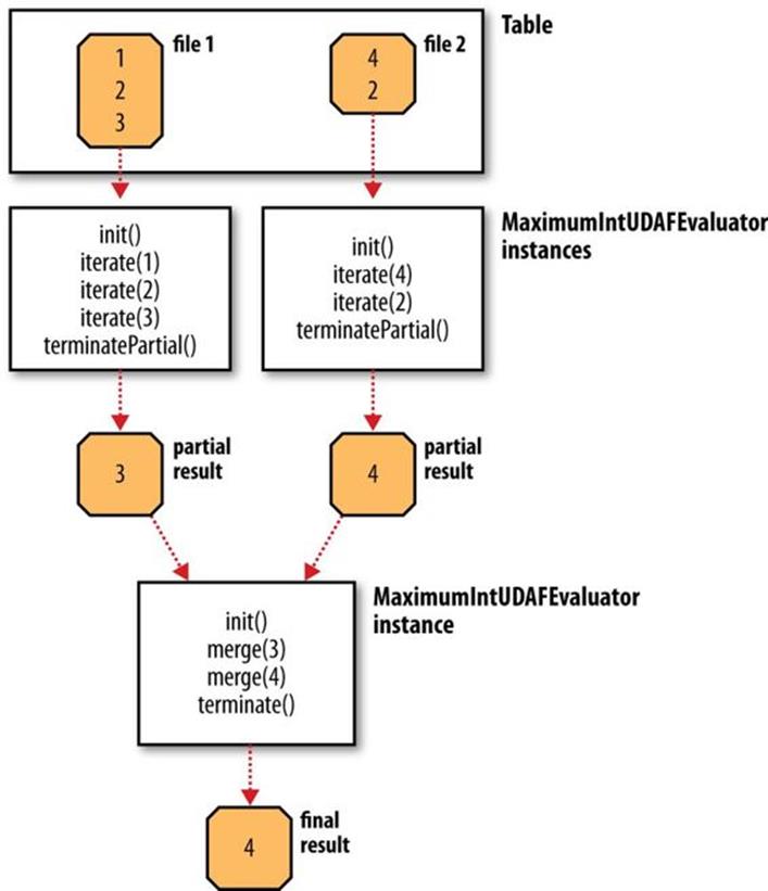
Figure 17-3. Data flow with partial results for a UDAF

A more complex UDAF

The previous example is unusual in that a partial aggregation can be represented using the same type (IntWritable) as the final result. This is not generally the case for more complex aggregate functions, as can be seen by considering a UDAF for calculating the mean (average) of a collection of double values. It’s not mathematically possible to combine partial means into a final mean value (see Combiner Functions). Instead, we can represent the partial aggregation as a pair of numbers: the cumulative sum of the double values processed so far, and the number of values.

This idea is implemented in the UDAF shown in Example 17-4. Notice that the partial aggregation is implemented as a “struct” nested static class, called PartialResult, which Hive is intelligent enough to serialize and deserialize, since we are using field types that Hive can handle (Java primitives in this case).

In this example, the merge() method is different from iterate() because it combines the partial sums and partial counts by pairwise addition. In addition to this, the return type of terminatePartial() is PartialResult — which, of course, is never seen by the user calling the function — whereas the return type of terminate() is DoubleWritable, the final result seen by the user.

Example 17-4. A UDAF for calculating the mean of a collection of doubles

package com.hadoopbook.hive;

import org.apache.hadoop.hive.ql.exec.UDAF;

import org.apache.hadoop.hive.ql.exec.UDAFEvaluator;

import org.apache.hadoop.hive.serde2.io.DoubleWritable;

public class Mean extends UDAF {

public static class MeanDoubleUDAFEvaluator implements UDAFEvaluator {

public static class PartialResult {

double sum;

long count;

}

private PartialResult partial;

public void init() {

partial = null;

}

public boolean iterate(DoubleWritable value) {

if (value == null) {

return true;

}

if (partial == null) {

partial = new PartialResult();

}

partial.sum += value.get();

partial.count++;

return true;

}

public PartialResult terminatePartial() {

return partial;

}

public boolean merge(PartialResult other) {

if (other == null) {

return true;

}

if (partial == null) {

partial = new PartialResult();

}

partial.sum += other.sum;

partial.count += other.count;

return true;

}

public DoubleWritable terminate() {

if (partial == null) {

return null;

}

return new DoubleWritable(partial.sum / partial.count);

}

}

}

Further Reading

For more information about Hive, see Programming Hive by Edward Capriolo, Dean Wampler, and Jason Rutherglen (O’Reilly, 2012).

^[106^] Toby Segaran and Jeff Hammerbacher, Beautiful Data: The Stories Behind Elegant Data Solutions (O’Reilly, 2009).

^[107^] It is assumed that you have network connectivity from your workstation to the Hadoop cluster. You can test this before running Hive by installing Hadoop locally and performing some HDFS operations with the hadoop fs command.

^[108^] The properties have the javax.jdo prefix because the metastore implementation uses the Java Data Objects (JDO) API for persisting Java objects. Specifically, it uses the DataNucleus implementation of JDO.

^[109^] Or see the Hive function reference.

^[110^] The move will succeed only if the source and target filesystems are the same. Also, there is a special case when the LOCAL keyword is used, where Hive will copy the data from the local filesystem into Hive’s warehouse directory (even if it, too, is on the same local filesystem). In all other cases, though, LOAD is a move operation and is best thought of as such.

^[111^] You can also use INSERT OVERWRITE DIRECTORY to export data to a Hadoop filesystem.

^[112^] However, partitions may be added to or removed from a table after creation using an ALTER TABLE statement.

^[113^] The fields appear to run together when displaying the raw file because the separator character in the output is a nonprinting control character. The control characters used are explained in the next section.

^[114^] The default format can be changed by setting the property hive.default.fileformat.

^[115^] Sometimes you need to use parentheses for regular expression constructs that you don’t want to count as a capturing group — for example, the pattern (ab)+ for matching a string of one or more ab characters. The solution is to use a noncapturing group, which has a ? character after the first parenthesis. There are various noncapturing group constructs (see the Java documentation), but in this example we could use (?:ab)+ to avoid capturing the group as a Hive column.

^[116^] This is a reworking in Hive of the discussion in Secondary Sort.

^[117^] The order of the tables in the JOIN clauses is significant. It’s generally best to have the largest table last, but see the Hive wiki for more details, including how to give hints to the Hive planner.