SQL Server Integration Services Design Patterns, Second Edition (2014)

Chapter 8. Loading a PDW Region in APS

SQL Server Parallel Data Warehouse (PDW) is Microsoft’s massively parallel processing (MPP) offering and is available as part of Microsoft’s Analytics Platform System (APS). APS is a turnkey solution focused on big data analytics. It offers two regions, or software options, to customers: PDW and HDInsight, which is Microsoft’s 100% Apache Hadoop distribution. PDW is built upon the SQL Server platform, although it is a separate product with a build of SQL Server specifically designed to support MPP operations.

Massively Parallel Processing

As the name suggests, massively parallel processing (MPP) uses multiple servers working as one system, called an appliance, to achieve much greater performance and scan rates than in traditional SMP systems. SMP refers to symmetric multiprocessing; most database systems, such as all other versions of SQL Server, are SMP.

To obtain a better understanding of the difference between SMP and MPP systems, let’s examine a common analogy. Imagine you are handed a shuffled deck of 52 playing cards and are asked to retrieve all of the queens. Even at your fastest, it would take you several seconds to retrieve the requested cards. Let’s now take that same deck of 52 cards and divide it among ten people. No matter how quick you are, these ten people working together can retrieve all of the queens much faster than you can by yourself.

As you may have inferred, you represent the SMP system, and the ten people represent the MPP system. This divide-and-conquer strategy is why MPP appliances are particularly well suited for high-volume, scan-intensive data warehousing environments, especially ones that need to scale to hundreds of terabytes—or even petabytes!—of storage. There are other MPP appliance vendors available besides Microsoft; however, the ability to easily join unstructured data in HDInsight with structured data in PDW via PolyBase, close integration with the Microsoft business intelligence stack (SQL Server, Integration Services, Analysis Services, and Reporting Services), and a compelling cost-per-terabyte makes APS a natural progression for organizations that need to take their SQL Server data warehouse to the next level. In this chapter, we will walk through how to efficiently load data into a PDW region in an APS appliance using Integration Services. But before we do that, we will first explore the architecture of APS. APS could easily consume a book in its own right, so we will only be covering the most pertinent parts to ensure that you have the foundation necessary for efficiently loading data into PDW.

Tip Learn more about Microsoft’s Analytics Platform System (APS), Parallel Data Warehouse (PDW), and HDInsight at http://microsoft.com/aps.

APS Appliance Overview

Generally, ETL developers and data integration engineers need not worry about the hardware specifications of the database systems they interact with. This isn’t the case when you are loading MPP systems. Because MPP systems are designed to take advantage of distributed data and parallelized workloads, you will find tremendous performance benefits in designing ETL solutions that take advantage of the parallelization units of an MPP system. For that reason, we will briefly review general hardware and software architectures for Microsoft’s APS appliance before we dive into load patterns.

Hardware Architecture

Microsoft has partnered and closely collaborated with Dell, HP, and Quanta to provide customers with a choice in hardware vendors. The hardware specifications of an APS appliance will vary depending on your chosen hardware vendor and capacity requirements, although there are some consistencies across the vendors.

Note For simplicity, we will examine APS configurations comprised only of PDW. It’s worth noting, however, that both PDW and HDInsight can run side-by-side in the same appliance through the use of separate hardware regions dedicated to each application. Microsoft calls this configuration a multi-region appliance.

The base rack is the smallest unit available for purchase and contains everything required to run a SQL Server PDW region. Depending on the hardware vendor, the minimum configuration will include either two or three Compute nodes. Similarly, the scale unit—that is, the number of compute nodes required to increase the capacity of the appliance—is dependent on vendor and will either be two or three Compute nodes. For all base racks, irrespective of hardware vendor, the top of the base rack includes the following:

· Two redundant InfiniBand switches

· Two redundant Ethernet switches

· One active server, which contains VMs for

· SQL Server PDW Control node

· Management and Active Directory

· Fabric Active Directory

· Hyper-V Virtual Machine Manager

· One passive spare server

The bottom of the base rack includes additional servers and storage. To add more storage or processing capacity, add scale units to the base rack until the base rack is full.

Note For simplicity and consistency, we will use depictions of Dell’s hardware configurations. However, please do not mistake that as an endorsement on the part of the authors. We suggest you review the offerings of each hardware vendor and make the selection that best meets your requirements.

Once the base rack is full, you can continue to add near-linear scalability to your APS appliance by adding one or more expansion racks. All expansion racks, irrespective of hardware vendor, are comprised of the following:

· Two redundant InfiniBand switches

· Two redundant Ethernet switches

· Scale units of either two or three Compute nodes

The expansion rack is very similar to the base rack. Just like the base rack, the bottom of the expansion rack includes servers and storage in scale units of either two or three Compute nodes. In fact, the only difference between the base rack and the expansion rack is the absence of the active server and optional spare server at the top of the rack.

Software Architecture

In the previous section, we discussed that the primary difference between the base rack and the expansion rack is the active server at the top of the rack. Let’s dig into that server in a little more detail.

The active server is comprised of four virtual machines (VMs) that provide functionality essential to the operation of the appliance. The four VMs are the PDW Control node (CTL), the Management and Active Directory (MAD), the Fabric Active Directory (AD), and Hyper-V Virtual Machine Manager (VMM). As an ETL developer or data integration engineer, you will only interact directly with the PDW Control node VM. Figure 8-1 depicts a nine-node rack and the four VMs that reside in the Active Server.

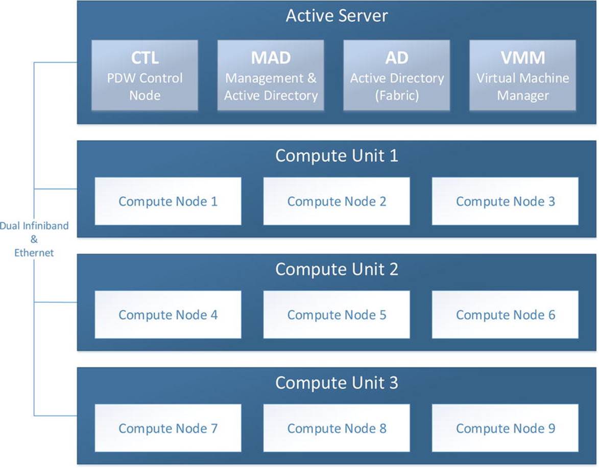
Figure 8-1. APS virtual machines

The PDW Control node VM provides the following critical functionality:

· Client connectivity and authentication

· System and database metadata

· SQL request processing

· Execution plan preparation

· Distributed execution orchestration

· Result aggregation

You can think of the Control node as the “brains” behind the distribution and parallelization of PDW. Although metadata resides on the Control node, no user data is persisted there. Rather, the Control node directs the loading and retrieval of user data to the appropriate Compute node and distribution. This is the first time we’ve introduced the term distribution, so if you’re not yet familiar with the term, don’t worry. We’ll cover distributions in the next section.

Shared-Nothing Architecture

At the core of PDW is the concept of shared-nothing architecture. In a shared-nothing architecture, a single logical table is broken up into numerous smaller physical pieces. The exact number of pieces depends on the number of Compute nodes in the PDW region. Within a single Compute node, each data piece is then split across eight (8) distributions. The number of distributions per Compute node cannot be configured and is consistent across all hardware vendors.

A distribution is the most granular physical level within PDW. Each distribution contains its own dedicated CPU, memory, and storage (LUNs), which it uses to store and retrieve data. Because each distribution contains its own dedicated hardware, it can perform load and retrieval operations in parallel with other distributions. This concept is what we mean by “shared-nothing.” There are numerous benefits that a shared-nothing architecture enables, such as more linear scalability. But perhaps PDW’s greatest power is its ability to scan data at incredible speeds.

Let’s do some math. Assume you have a PDW appliance with a base rack containing 9 Compute nodes, and you need to store a table with 1 billion rows. The data will be split across all 9 Compute nodes, and each Compute node will split its data across 8 distributions. Thus, the 1-billion-row table will be split into 72 distributions (9 Compute nodes × 8 distributions per Compute node). That means each distribution will store roughly 13,900,000 rows.

But what does this mean from the end user’s standpoint? Let’s look at a hypothetical situation. You are a user at a retail company and you have a query that joins two tables together: a Sales table with 1 billion rows, and a Customer table with 50 million rows. And, as luck would have it, there are no indexes available that will cover your query. This means you will need to scan, or read, every row in each table.

In an SMP system—where memory, storage, and CPU are shared—this query could take hours or days to run. On some systems, it might not even be feasible to attempt this query, depending on factors such as the server hardware and the amount of activity on the server. Suffice it to say, the query will take a considerable amount of time to return and will most likely have a negative impact on other activity on the server.

In PDW, these kinds of queries often return in minutes, and a well-designed schema, where the rows you’re joining are stored together on the same distribution, can even execute this query in seconds. This is because the architecture is optimized for scans; PDW expects to scan every row in the table. Remember how we said that every distribution has its own dedicated CPU, memory, and storage? When you submit the query to join 1 billion rows to 50 million rows, each distribution is performing a scan on its own Sales table of 13,800,000 rows and Customer table with 695,000 rows. These smaller volumes are much more manageable, and an idle distribution can handle this workload with ease. The data is then sent back to the Control node across an ultra-fast dual-InfiniBand channel to consolidate the results and return the data to the end user. It is this divide-and-conquer strategy that allows PDW to significantly outperform SMP systems.

Clustered Columnstore Indexes

Columnstore refers to the storing of data in a columnar—or column-oriented—storage format. In traditional RDBMS systems, data is stored using a rowstore—or row-oriented—storage format. Rowstores are generally well suited for transactional applications where the application is concerned with most or all columns for one or a small number of rows. Columnstores, on the other hand, are better suited for analytical applications, which are generally concerned with a subset of columns and a large portion, or even all, of the rows in the table.

For those of you familiar with indexing in SQL Server, you may think of a clustered columnstore index (CCI) as analogous to a clustered index in a row-oriented table. But unlike a clustered index, once a CCI has been defined, additional indexes such as nonclustered indexes may not be created on that table.

CCIs offer several performance improvements over traditional rowstores in PDW. Some customers have seen up to ten times the query performance and up to seven times the data compression improvements. Because of the compression and related performance improvements, Microsoft recommends CCI as the standard storage format for tables in PDW.

Tip Columnstores are available in both PDW and SQL Server Enterprise Edition. For more information on columnstore indexes, refer to the “Columnstore Indexes Described” topic on MSDN, or navigate to http://msdn.microsoft.com/en-us/library/gg492088.

Loading Data

We discussed in the previous section that PDW is able to query data very efficiently because of its shared-nothing architecture. For the same reason, PDW is also able to load data very efficiently. Let’s briefly discuss how PDW can perform data imports so efficiently.

As previously mentioned, the Control VM is the first stop for anything being written or retrieved from the appliance. The Control node determines which Compute nodes will be involved in the storage operation. Each Compute node then uses a hashing algorithm to determine where to store the data, down to the individual distribution and associated LUNs. This allows each distribution to load its data in parallel with other distributions. Again, dividing and conquering a large table import in parallel will be much faster than performing a single large import or performing several smaller imports serially.

Data can be imported from numerous platforms, including from Oracle, SQL Server, MySQL, and flat files. There are two primary methods of loading data into the PDW appliance: DWLoader and Integration Services. We will briefly discuss when to use DWLoader vs. Integration Services. After that, we will walk through an example of loading data from SQL Server using Integration Services.

DWLoader vs. Integration Services

DWLoader is a command-line utility that ships with PDW. Those familiar with SQL Server BCP (bulk copy program) will have an easy time learning DWLoader, because both utilities share a very similar syntax. One very common pattern for loading data into PDW from SQL Server is to

1. Export data from SQL Server to a flat file using BCP.

2. Store the flat file on the loading server.

3. Import the data file from the loading server to PDW using DWLoader.

This is a very efficient method for importing data, and it is very easy to generate scripts for table DDL, BCP commands, and DWLoader commands. For this reason, you may want to consider DWLoader for performing initial and incremental loading of the large quantity of small dimensional tables that often exist in data warehouses. Doing so can greatly speed up a data warehouse migration. This same load pattern can also be used with flat files generated from any system, not just SQL Server.

For your larger tables, you may instead want to consider Integration Services. Integration Services offers greater functionality and arguably more end-to-end convenience. This is because Integration Services is able to connect directly to the data source and load the data into the PDW appliance without having to stop at a file share. Another important distinction is that Integration Services can also perform transformations in flight, which DWLoader does not support.

It’s worth noting that each data flow within Integration Services is single-threaded and can bottleneck on I/O. Typically, a single-threaded Integration Services package will perform up to ten times slower than DWLoader. However, a multithreaded Integration Services package—similar to the one we will create shortly—can mitigate that limitation. For large tables requiring data type conversions, an Integration Services package with ten parallel data flows provides the best of both worlds: similar performance to DWLoader and all the advanced functionality that Integration Services offers.

You should consider a number of variables when deciding whether to use DWLoader or Integration Services. In addition to table size, both network speed and table design can have an impact. At the end of the day, most PDW implementations will likely use a combination of both tools. The best idea is to test the performance of each method in your environment and use the tool that makes the most sense for each table pattern.

ETL vs. ELT

Many Integration Services packages are designed using an extract, transform, and load (ETL) process. This is a practical model that strives to lessen the impact of moving data on the source and destination servers, which are traditionally more resource-constrained, by placing the burden of data filtering, cleansing, and other such activities on the (arguably more easy-to-scale) ETL server. Extract, load, and transform (ELT) processes, in contrast, place the burden on the destination server.

Although both models have their place and PDW supports both, ELT makes more sense with PDW from both a technical and a business perspective. On the technical side, PDW is able to utilize its massively parallel processing (MPP) power to more efficiently load and transform large volumes of data. From the business aspect, having more data co-located allows more meaningful data to be gleaned during the transformation process. Organizations with MPP systems often find that the ability to co-locate and transform large quantities of disparate data enables them to make the leap from reactive data marts (How much of this product did we sell?) to predictive data modeling (How can we sell more of this product?).

Just because you have decided on an ELT strategy does not necessarily mean your Integration Services package will not have to perform any transformations. In fact, many Integration Services packages may require data type transformations. Table 8-1 illustrates the data types supported in PDW and the equivalent Integration Services data types.

Table 8-1. Data Type Mappings for PDW and Integration Services

Also, it is worth noting that PDW does not currently support the following data types at the time of this writing:

· DT_DBTIMESTAMPOFFSET

· DT_DBTIME2

· DT_GUID

· DT_IMAGE

· DT_NTEXT

· DT_TEXT

Any of these unsupported data types will need to be converted to a compatible data type using the Data Conversion transformation. We will walk through how to perform such a transformation in just a moment.

Data Import Pattern for PDW

Now that you have a basic understanding of the architecture and loading concepts of an APS appliance, we’re ready to get started with the pattern for importing data into PDW.

Prerequisites

All Integration Services packages will be executed from a loading server. A loading server is a non-appliance server that resides on your network and runs Windows Server 2008 R2 or newer. The loading server is connected to the APS appliance via Ethernet or InfiniBand, the latter of which is recommended for better performance. Additionally, the loading server will require permissions to access the Control node and must have Integration Services and the PDW destination adapter installed.

The requirements for the PDW destination adapter will vary depending on the version of PDW and Integration Services you are running. The PDW documentation outlines the various requirements and installation instructions in great detail. Please refer to the “Install Integration Services Destination Adapters (SQL Server PDW)” section of your PDW documentation for more information.

Once the PDW destination adapter is installed on the loading server, we’re ready to create mock data.

Preparing the Data

In preparation for moving data from SQL Server to PDW, you need to create a database in SQL Server and populate it with some test data. Execute the T-SQL code in Listing 8-1 from your favorite query editor, such as SQL Server Management Studio (SSMS), to create a new database calledPDW_Example.

Listing 8-1. Example of T-SQL Code to Create a SQL Server Database

USE [master];
GO

/* Create a database to experiment with */
CREATE DATABASE [PDW_Example]
ON PRIMARY
(
NAME = N'PDW_Example'
, FILENAME = N'C:\Program Files\Microsoft SQL Server\MSSQL12.MSSQLSERVER\ MSSQL\DATA\PDW_Example.mdf'
, SIZE = 1024MB
, MAXSIZE = UNLIMITED
, FILEGROWTH = 1024MB
)
LOG ON
(
NAME = N'PDW_Example_Log'
, FILENAME = N'C:\Program Files\Microsoft SQL Server\MSSQL12.MSSQLSERVER\ MSSQL\DATA\PDW_Example_Log.ldf'
, SIZE = 256MB
, MAXSIZE = UNLIMITED
, FILEGROWTH = 256MB
);
GO

Please note that your database file path will vary depending on the details of your particular installation.

Next, create a table and populate it with some data. As we discussed before, Integration Services works best with large tables that can be multithreaded. One good example of this is a Sales Fact table that is partitioned by year. Listing 8-2 will provide the T-SQL code you need to create the table and partitioning dependencies.

Listing 8-2. Example of T-SQL Code to Create a Partitioned Table in SQL Server

USE PDW_Example;
GO

/* Create your partition function */
CREATE PARTITION FUNCTION example_yearlyDateRange_pf
(DATETIME) AS RANGE RIGHT
FOR VALUES('2013-01-01', '2014-01-01', '2015-01-01');
GO

/* Associate your partition function with a partition scheme */
CREATE PARTITION SCHEME example_yearlyDateRange_ps
AS PARTITION example_yearlyDateRange_pf ALL TO([Primary]);
GO

/* Create a partitioned fact table to experiment with */
CREATE TABLE PDW_Example.dbo.FactSales (
orderID INT IDENTITY(1,1)
, orderDate DATETIME
, customerID INT
, webID UNIQUEIDENTIFIER DEFAULT (NEWID())

CONSTRAINT PK_FactSales
PRIMARY KEY CLUSTERED
(
orderDate
, orderID
)
) ON example_yearlyDateRange_ps(orderDate);

Note Getting an error on the above syntax? Partitioning is a feature only available in SQL Server Enterprise and Developer Editions. If you are not using Enterprise or Developer Editions, you can comment out the partitioning in the last line

ON example_yearlyDateRange_ps(orderDate);

and replace it with

ON [Primary];

Next, you need to generate data using the T-SQL in Listing 8-3. This is the data you will be loading into PDW.

Listing 8-3. Example of T-SQL Code to Populate a Table with Sample Data

/* Declare variables and initialize with an arbitrary date */
DECLARE @startDate DATETIME = '2013-01-01';

/* Perform an iterative insert into the FactSales table */
WHILE @startDate < '2016-01-01'
BEGIN

INSERT INTO PDW_Example.dbo.FactSales (orderDate, customerID)
SELECT @startDate
, DATEPART(WEEK, @startDate) + DATEPART(HOUR, @startDate);

/* Increment the date value by hour; for more test data,
replace HOUR with MINUTE or SECOND */
SET @startDate = DATEADD(HOUR, 1, @startDate);

END;

This script will generate roughly 26,000 rows in the FactSales table spanning 3 years, although you can easily increase the number of rows generated by replacing HOUR in the DATEADD statement with MINUTE or even SECOND.

Now that you have a data source to work with, you are ready to start working on your Integration Services package.

Package Overview

Let’s discuss what your package will do. You are going to configure a data flow that will move data from SQL Server to PDW. You will create a connection to your data source via an OLE DB Source. Because UNIQUEIDENTIFIER (also known as a GUID) is not yet supported as a data type in PDW, you will transform the UNIQUEIDENTIFIER to a Unicode string (DT_WSTR) using a data conversion. You will then configure the PDW destination adapter to load data into the APS appliance. Lastly, you will multithread the package, which takes advantage of PDW’s parallelization to improve load performance.

One easy way to multithread is to create multiple data flows that execute in parallel for the same table. You can have up to ten simultaneous loads—ten data flows—for a table. The challenge with simultaneous loading, however, is to avoid causing too much contention on the source system. You can minimize contention by isolating each data flow to a separate, equal portion of the clustered index. Better yet, if you have SQL Server Enterprise Edition, you can isolate each data flow by loading by partition. This latter method is preferable and is the approach our example will use.

Now that you understand the general structure of the Integration Services package, let’s create it.

The Data Source

If you have not already done so, create a new Integration Services project named PDW_Example (File New Project Integration Services Project).

Add a Data Flow task to the control flow designer surface. Name it PDW Import.

Add an OLE DB Source to the designer surface from the SSIS Toolbox. Edit the properties of the OLE DB Source by double-clicking on the icon. You should see the source editor shown in Figure 8-2.

Figure 8-2. The OLE DB Source Editor

You will need to create an OLE DB Connection Manager that points to the PDW_Example database. Once this is done, change the data access mode to SQL Command; then enter the code in Listing 8-4.

Listing 8-4. Example SQL Command

/* Retrieve sales for 2013 */

SELECT
orderID
, orderDate
, customerID
, webID
FROM PDW_Example.dbo.FactSales
WHERE orderDate >= '2013-01-01'
AND orderDate < '2014-01-01';

Your OLE DB Source Editor should look similar to Figure 8-2. Click Preview to verify the results, then click OK to close the editor.

This code is simple, but it’s doing something pretty important. By searching the FactSales table on orderDate—the column specified as the partitioning key in Listing 8-2—SQL Server is able to perform partition elimination, which is important for minimizing I/O contention. This provides a natural boundary for each data flow that is both easy to understand and performs well. You can achieve a similar result even without partitioning FactSales by performing a sequential seek on the clustered index, orderDate. But what if FactSales was clustered on justorderID instead? You can apply the same principles and achieve good performance by searching for an evenly distributed number of sequential rows in each data flow. For example, if FactSales has 1,000,000 rows and we are using 10 data flows, each OLE DB Source should search for 100,000 rows (i.e., orderID >= 1 and orderID < 100000; orderID >= 100000 and orderID < 200000; and so on). These types of design considerations can have a significant impact on the overall performance of your Integration Services package.

Tip Not familiar with partitioning? Table partitioning is particularly well suited for large data warehouse environments and offers more than just the benefits briefly mentioned here. More information is available in the whitepaper, “Partitioned Table and Index Strategies Using SQL Server 2008,” at http://msdn.microsoft.com/en-us/library/dd578580.aspx.

The Data Transformation

As you may recall, the source table has a UNIQUEIDENTIFIER column that is stored as a CHAR(38) column in PDW. In order to load this data, we will need to transform the UNIQUEIDENTIFER to a Unicode string. To do this, drag the Data Conversion icon from the SSIS Toolbox to the designer surface. Next, connect the blue data flow arrow from OLE DB Source to Data Conversion, as shown in Figure 8-3.

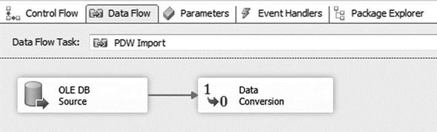
Figure 8-3. Connecting the OLE DB Source to the Data Conversion

Double-click on the Data Conversion icon to open the Data Conversion Transformation Editor. Click on the box to the left of webID; then edit its properties to reflect the following values:

· Input Column: webID

· Output Alias:

· Data Type: string [DT_WSTR]

· Length: 38

Confirm that the settings match those in Figure 8-4, then click OK.

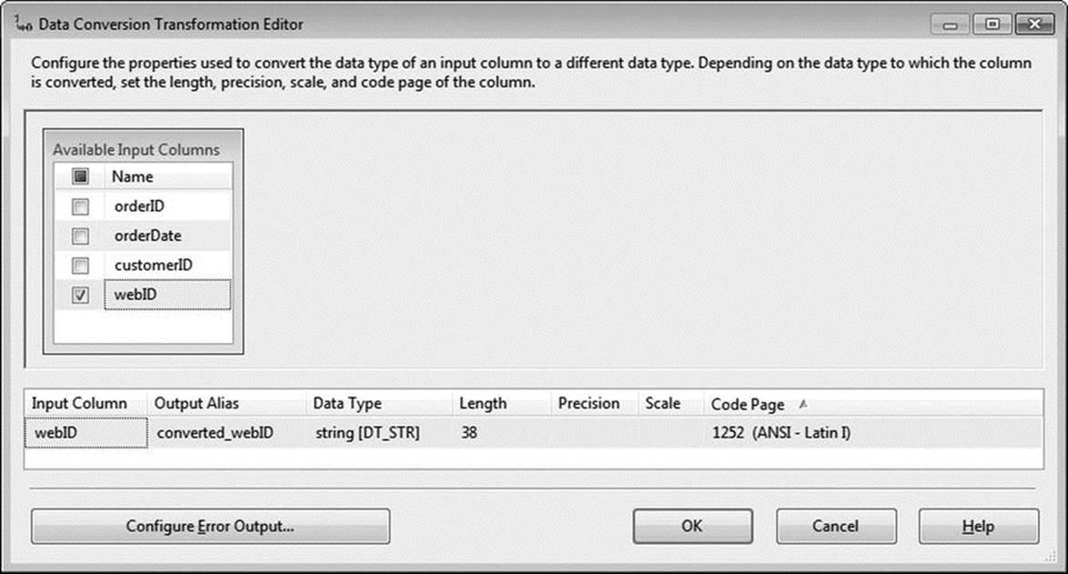
Figure 8-4. The Data Conversion Transformation Editor

Tip Wonder why we use a string length of 38 when converting a UNIQUEIDENTIFIER to a CHAR? This is because the global representation of a GUID is {00000000-0000-0000-0000-000000000000}. The curly brackets are stored implicitly in SQL Server forUNIQUEIDENTIFIER columns. Thus, during conversion, Integration Services materializes the curly brackets for export to the destination system. That is why, although a UNIQUEIDENTIFIER may look like it would only consume 36 bytes, it actually requires 38 bytes to store in PDW.

The Data Destination

The next few tasks, which prepare the PDW appliance for receiving FactSales data, will take place in SQL Server Data Tools—or just SSDT for short. Please refer to the section, “Install SQL Server Data Tools for Visual Studio (SQL Server PDW),” in the PDW documentation for more information on connecting to PDW from SSDT.

Before we go any further, we should discuss the use of a staging database. Although it is not required, Microsoft recommends that you use a staging database during incremental loads to reduce table fragmentation. When you use a staging database, the data is first loaded into a temporary table in the staging database before it is inserted into the permanent table in the destination database.

Tip Using a staging database? Make sure your staging database has enough space available to accommodate all tables being loaded concurrently. If you do not allocate enough space initially, don’t worry; you’ll still be okay—the staging database will autogrow. Your loads may just slow down while the autogrow is occurring. Also, your staging database will likely need to be larger when you perform the initial table loads during system deployment and migration. However, once your system becomes more mature and the initial ramp-up is complete, you can recover some space by dropping and re-creating a smaller staging database.

From within SSDT, execute the code in Listing 8-5 on your PDW appliance to create a staging database.

Listing 8-5. PDW Code to Run from SSDT to Create a Staging Database

CREATE DATABASE StageDB_Example
WITH
(
AUTOGROW = ON
, REPLICATED_SIZE = 1 GB
, DISTRIBUTED_SIZE = 5 GB
, LOG_SIZE = 1 GB
);

PDW introduces the concept of replicated and distributed tables. In a distributed table, the data is split across all nodes using a distribution hash specified during table creation. In a replicated table, the full table data exist on every Compute node. When used correctly, a replicated table can often improve join performance. As a hypothetical example, consider a small DimCountry dimension table with 200 rows. DimCountry would likely be replicated, whereas a much larger FactSales table would be distributed. This design allows any joins between FactSalesand DimCountry to take place locally on each node. Although you would essentially be creating ten copies of DimCountry, one on each Compute node, the performance benefit of a local join outweighs the minimal cost of storing duplicate copies of such a small table.

Let’s take another look at the CREATE DATABASE code in Listing 8-5. REPLICATED_SIZE specifies space allocation for replicated tables on each Compute node, whereas DISTRIBUTED_SIZE specifies space allocation for distributed tables across the appliance. That meansStageDB_Example actually has 16GB of space allocated: 10GB for replicated tables (10 Compute nodes with 1GB each), 5GB for distributed tables, and 1GB for the log.

All data is automatically compressed using page-level compression during the PDW load process. This is not optional, and the amount of compression will vary greatly from customer to customer and table to table. If you have SQL Server Enterprise or Developer Editions, you can execute the statement in Listing 8-6 to estimate compression results.

Listing 8-6. Code to Estimate Compression Savings

/* Estimate compression ratio */
EXECUTE sp_estimate_data_compression_savings
'dbo', 'FactSales', NULL, NULL, 'PAGE';

Example results of sp_estimate_data_compression_savings are shown in Figure 8-5.

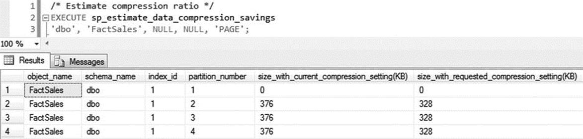
Figure 8-5. Example compression savings

You can generally use 2:1 as a rough estimate. With a 2:1 compression ratio, the 5GB of distributed data specified in Listing 8-5 actually stores 10GB of uncompressed SQL Server data.

You still need a place in PDW to store the data you’re importing. Execute the code in Listing 8-7 in SSDT to create the destination database and table for FactSales.

Listing 8-7. PDW Code to Create the Destination Database and Table

CREATE DATABASE PDW_Destination_Example
WITH
(
REPLICATED_SIZE = 1 GB
, DISTRIBUTED_SIZE = 5 GB
, LOG_SIZE = 1 GB
);

CREATE TABLE PDW_Destination_Example.dbo.FactSales
(
orderID INT
, orderDate DATETIME
, customerID INT
, webID CHAR(38)
)
WITH
(
DISTRIBUTION = HASH (orderID)
, CLUSTERED COLUMNSTORE INDEX
);

Now that the destination objects are created, we can return to the Integration Services package. Drag the SQL Server PDW Destination from the Toolbox to the Data Flow pane. Double-click on the SQL Server PDW Destination, illustrated in Figure 8-6, to edit its configuration.

Figure 8-6. The SQL Server PDW Destination

Next, click on the down arrow next to Connection Manager and select <Create New Connection. . .>, as shown in Figure 8-7.

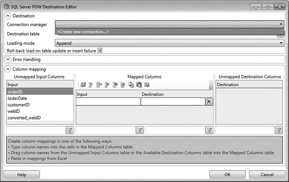
Figure 8-7. The SQL Server PDW Destination Editor

Enter your connection information in the SQL Server PDW Connection Manager Editor using these items:

· Server: The IP address of the Control node on your appliance (Best practice is to use the clustered IP address to support Control node failover.)

· User: Your login name for authenticating to the appliance

· Password: Your login password

· Destination Database: PDW_Destination_Example

· Staging Database: StageDB_Example

Let’s discuss a few best practices relating to this connection information. First, you should specify the IP address of the Control node cluster instead of the IP address of the active Control node server. Using the clustered IP address will allow your connection to still resolve without manual intervention in the event of a Control node failover.

Secondly, PDW supports both SQL Server and Active Directory authentication. When using SQL Server authentication, best practice is to use an account other than sa. Doing so will improve the security of your PDW appliance.

Lastly, as we previously discussed, Microsoft recommends the use of a staging database for data loads. The staging database is selected in the Staging Database Name drop-down. This tells PDW to first load the data to a temporary table in the specified staging database before loading the data into the final destination database. This is optional, but loading directly into the destination database will increase fragmentation.

When you are done, your SQL Server PDW Connection Manager Editor should resemble Figure 8-8. Click on Test Connection to confirm your information was entered correctly, then click OK to return to the SQL Server PDW Destination Editor.

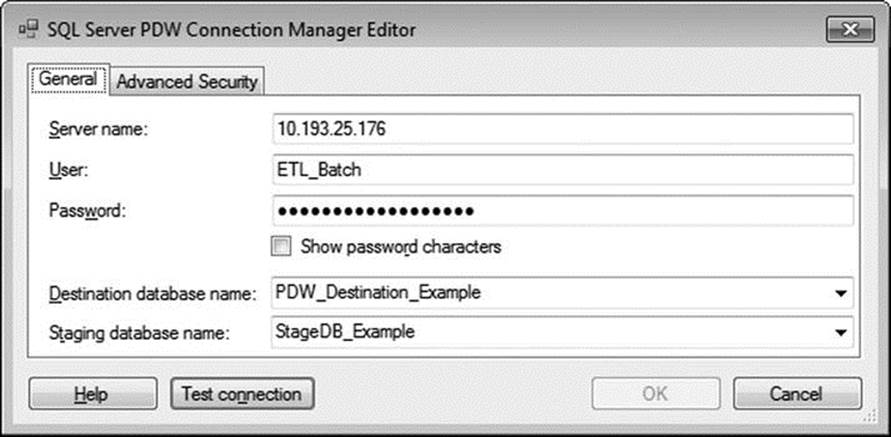
Figure 8-8. The SQL Server PDW Connection Manager Editor

Note If the staging database is not specified, SQL Server PDW will perform the load operation directly within the destination database, which can lead to high levels of table fragmentation.

Clicking on the Destination Table field will bring up a model for Select Destination Table. Click on FactSales. There are four loading modes available:

· Append: Inserts the rows at the end of existing data in the destination table. This is the mode you are probably most used to.

· Reload: Truncates the table before load.

· Upsert: Performs a MERGE on the destination table, where new data is inserted and existing data is updated. You will need to specify one or more columns that will be used to join the data.

· FastAppend: As its name implies, FastAppend is the fastest way to load data into a destination table. The trade-off is that it does not support rollback; in the case of a failure, you are responsible for removing any partially inserted rows. FastAppend will also bypass the staging database, causing high levels of fragmentation.

Let’s take a moment to discuss how to use these modes with two common load patterns. If you are performing regular, incremental loads on a large table (say, updating a transactional sales table with the previous day’s orders), you should load the data directly using Append, since no transformations are required. Now let’s say you’re loading the same data, but you plan to instead transform the data and load into a mart before deleting the temporary data. This second example would be better suited to the FastAppend mode. Or, to say it more concisely, use FastAppend any time you are loading into an empty, intermediate working table.

There is one last option we need to discuss. Underneath the Loading Mode is a checkbox for Roll-Back Load on Table Update or Insert Failure. In order to understand this option, you need to understand a little about how data is loaded into PDW. When data is loaded using the Append, Reload, or Upsert modes, PDW performs a two-phase load. In Phase 1, the data is loaded into the staging database. In Phase 2, PDW performs an INSERT/SELECT of the sorted data into the final destination table. By default, data is loaded in parallel on all Compute nodes, but it is loaded serially within a Compute node to each distribution. This is necessary in order to support rollback. Roughly 85–95% of the load process is spent in Phase 1. When Roll-Back Load on Table Update or Insert Failure is deselected, each distribution is loaded in parallel instead of serially during Phase 2. So, in other words, deselecting this option will improve performance but only affects 5–15% of the overall process. Also, deselecting this option removes PDW’s ability to roll back; in the event of a failure during Phase 2, you would be responsible for cleaning up any partially inserted data.

Because of the potential risk and minimal gain, it is best practice to deselect this option only when you are loading to an empty table. FastAppend is unaffected by this option because it always skips Phase 2 and loads directly into the final table, which is why FastAppend also does not support rollback.

Tip Roll-Back Load on Table Update or Insert Failure is also available in DWLoader using the –m option.

Return to the PDW Destination Editor and select Append in the Loading Mode field. Because the destination table is currently empty, deselect the Roll-Back Load on Table Update or Insert Failure option to receive a small, risk-free performance boost.

You are almost done with your first data flow. All you have left to do is to map your data. Drag the blue arrow from the Data Conversion box to the SQL Server PDW Destination box, and then double-click on SQL Server PDW Destination. Map your input and destination columns. Make sure to map webID to your transformed converted_webID column. Click OK.

You have now successfully completed your first data flow connecting SQL Server to PDW. All you have left is to multithread the package.

Multithreading

You have completed the data flow for 2013, but you still need to create identical data flows for 2014 and 2015. You can do this easily by using copy and paste.

First, click on the Control Flow tab and rename the first Data Flow SalesMart 2013. Then, copy and paste the first data flow and rename it SalesMart 2014.

Double-click on SalesMart 2014 to return to the Data Flow designer, then double-click on the OLE DB Source. Replace the SQL Command with the code in Listing 8-8.

Listing 8-8. SQL Command for 2014 Data

/* Retrieve sales for 2014 */
SELECT
orderID
, orderDate
, customerID
, webID
FROM PDW_Example.dbo.FactSales
WHERE orderDate >= '2014-01-01'
AND orderDate < '2015-01-01';

Return to the Control Flow tab and copy the SalesMart 2013 data flow again. Rename it Sales Mart 2015. Using the code in Listing 8-9, replace the SQL command in the OLE DB Source.

Listing 8-9. SQL Command for 2015 Data

/* Retrieve sales for 2015 */
SELECT
orderID
, orderDate
, customerID
, webID
FROM PDW_Example.dbo.FactSales
WHERE orderDate >= '2015-01-01'
AND orderDate < '2016-01-01';

You are now ready to execute the package! Press F5 or navigate to Debug Start Debugging. Your package should execute, and you should see a successful result.

Limitations

ETL developers and data integration engineers should be aware of the following limitations and behaviors in PDW when developing ETL solutions:

· PDW is limited to a maximum of ten (10) active, concurrent loads. This number applies to the appliance as a whole, regardless of the number of Compute nodes, and cannot be changed.

· Each PDW destination adapter defined in an Integration Services package counts as one concurrent load. An Integration Services package with more than ten PDW destination adapters defined will not execute.

· As previously mentioned, not all SQL Server data types are supported in PDW. Refer to the list in Table 8-1 under “ETL vs. ELT,” or in your PDW documentation, for more details.

A small amount of overhead is associated with each load operation. This overhead is a necessary part of operating in a distributed environment. For example, the loading server needs to communicate with the Control node to identify which Compute nodes should receive data. Because this overhead is incurred on every single load, transactional load patterns (such as singleton inserts) should be avoided. PDW performs at its best when data is loaded in large, incremental batches. You will see much better performance loading 10 files with a 100,000 rows each, or a single file with 1,000,000 rows, than loading 1,000,000 rows individually.

Summary

We’ve covered a lot of material in this chapter. You have learned about the architectures of Microsoft’s Analytics Platform System (APS) and SQL Server Parallel Data Warehouse (PDW). You’ve learned about the differences between SMP and MPP systems and why MPP systems are better suited for large analytical workloads. You have learned about different methods for loading PDW and ways to improve load performance. You have also discovered some best practices along the way. Lastly, you walked through a step-by-step exercise to parallelize loading data from SQL Server into PDW using SSIS.