Professional Microsoft SQL Server 2014 Integration Services (Wrox Programmer to Programmer), 1st Edition (2014)
Chapter 12. Loading a Data Warehouse
WHAT’S IN THIS CHAPTER?
· Data profiling
· Dimension and fact table loading
· Analysis Services cube processing
WROX.COM DOWNLOADS FOR THIS CHAPTER
You can find the wrox.com code downloads for this chapter at www.wrox.com/go/prossis2014 on the Download Code tab.
Among the various applications of SQL Server Integration Services (SSIS), one of the more common is loading a data warehouse or data mart. SSIS provides the extract, transform, and load (ETL) features and functionality to efficiently handle many of the tasks required when dealing with transactional source data that will be extracted and loaded into a data mart, a centralized data warehouse, or even a master data management repository, including the capabilities to process data from the relational data warehouse into SQL Server Analysis Services (SSAS) cubes.
SSIS provides all the essential elements of data processing — from your source, to staging, to your data mart, and onto your cubes (and beyond!). A few common architectures are prevalent in data warehouse solutions. Figure 12-1 highlights one common architecture of a data warehouse with an accompanying business intelligence (BI) solution.
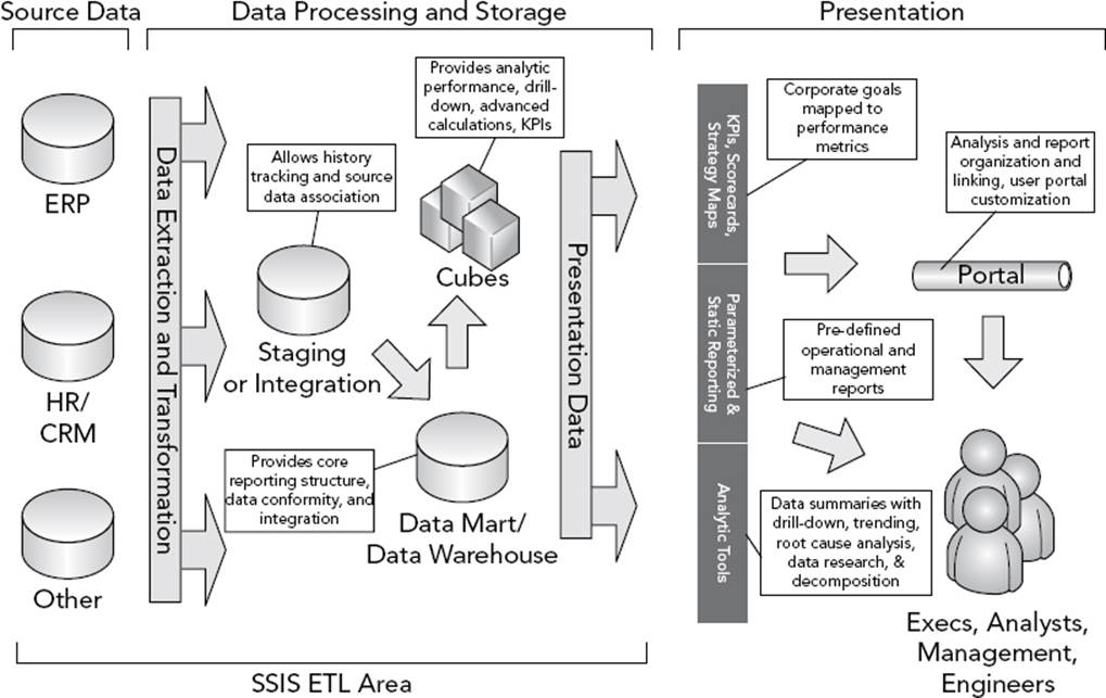
FIGURE 12-1
The presentation layer on the right side of Figure 12-1 shows the main purpose of the BI solution, which is to provide business users (from the top to the bottom of an organization) with meaningful data from which they can take actionable steps. Underlying the presentation data are the back-end structures and processes that make it possible for users to access the data and use it in a meaningful way.
Another common data warehouse architecture employs a central data warehouse with subject-oriented data marts loaded from the data warehouse. Figure 12-2 demonstrates this data warehouse architecture.
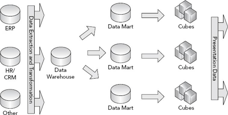
FIGURE 12-2
ETL is an important part of a data warehouse and data mart back-end process because it is responsible for moving and restructuring the data between the data tiers of the overall BI solution. This involves many steps, as you will see — including data profiling, data extraction, dimension table loading, fact table processing, and SSAS processing.
This chapter will set you on course to architecting and designing an ETL process for data warehouse and business intelligence ETL. In fact, SSIS contains several out-of-the-box tasks and transformations to get you well on your way to a stable and straightforward ETL process. Some of these components include the Data Profiling Task, the Slowly Changing Dimension Transformation, and the Analysis Services Execute DDL Task. The tutorials in this chapter, like other chapters, use the sample databases for SQL Server, called AdventureWorks and AdventureWorksDW. In addition to the databases, a sample SSAS cube database solution is also used. These databases represent a transactional database schema and a data warehouse schema. The tutorials in this chapter use the sample databases and demonstrate a coordinated process for the Sales Quota Fact table and the associated SSAS measure group, which includes the ETL required for the Employee dimension. You can go to www.wrox.com/go/prossis2014 and download the code and package samples found in this chapter, including the version of the SSAS AdventureWorks database used.
DATA PROFILING
Ultimately, data warehousing and BI is about reporting and analytics, and the first step to reach that objective is understanding the source data, because that has immeasurable impact on how you design the structures and build the ETL.
Data profiling is the process of analyzing the source data to better understand its condition in terms of cleanliness, patterns, number of nulls, and so on. In fact, you probably have profiled data before with scripts and spreadsheets without even realizing that it was called data profiling.
A helpful way to data profile in SSIS, the Data Profiling Task, is reviewed in Chapter 3, but let’s drill into some more details about how to leverage it for data warehouse ETL.
Initial Execution of the Data Profiling Task
The Data Profiling Task is unlike the other tasks in SSIS because it is not intended to be run repeatedly through a scheduled operation. Consider SSIS as the wrapper for this tool. You use SSIS to configure and run the Data Profiling Task, which outputs an XML file with information about the data you select. You then observe the results through the Data Profile Viewer, which is a standalone application. The output of the Data Profiling Task will be used to help you in your development and design of the ETL and dimensional structures in your solution. Periodically, you may want to rerun the Data Profiling task to see how the data has changed, but the task will not run in the recurring ETL process.
1. Open Visual Studio and create a new SSIS project called ProSSIS_Ch12. You will use this project throughout this chapter.
2. In the Solution Explorer, rename Package.dtsx to Profile_EmployeeData.dtsx.
3. The Data Profiling Task requires an ADO.NET connection to the source database (as opposed to an OLE DB connection). Therefore, create a new ADO.NET connection in the Connection Manager window by right-clicking and choosing “New ADO.NET Connection” and then click the New button. After you create a connection to the AdventureWorks database, return to the Solution Explorer window.
4. In the Solution Explorer, create a new project connection to your local machine or where the AdventureWorks sample database is installed, as shown in Figure 12-3.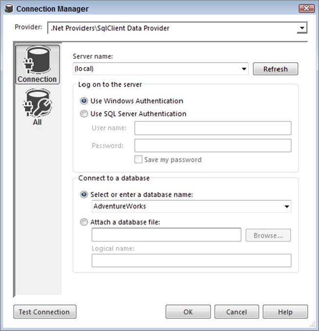
FIGURE 12-3
5. Click OK to save the connection information and return to the SSIS package designer. (In the Solution Explorer, rename the project connection to ADONETAdventureWorks.conmgr so that you will be able to distinguish this ADO.NET connection from other connections.)
6. Drag a Data Profiling Task from the SSIS Toolbox onto the Control Flow and double-click the new task to open the Data Profiling Task Editor.
7. The Data Profiling Task includes a wizard that will create your profiling scenario quickly; click the Quick Profile Button on the General tab to launch the wizard.
8. In the Single Table Quick Profile Form dialog, choose the ADONETAdventureWorks connection; and in the Table or View dropdown, select the [Sales].[vSalesPerson] view from the list. Enable all the checkboxes in the Compute list and change the Functional Dependency Profile to use 2 columns as determinant columns, as shown in Figure 12-4. The next section reviews the results and describes the output of the data profiling steps.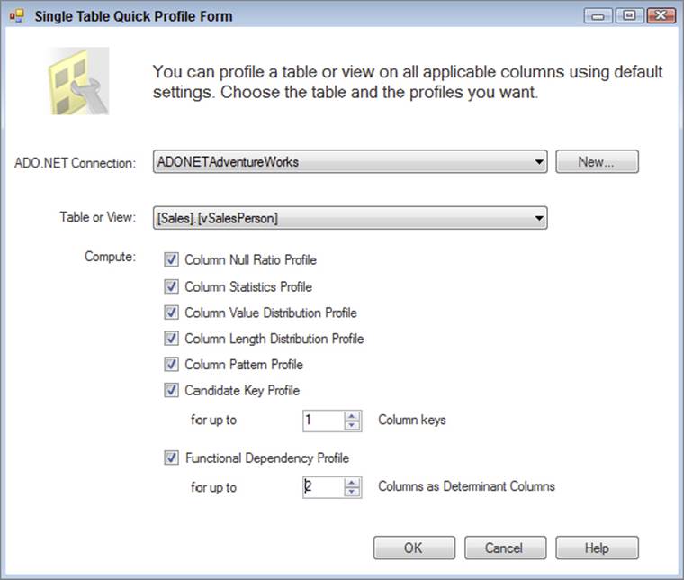
FIGURE 12-4
9. Click OK to save the changes, which will populate the Requests list in the Data Profiling Task Editor, as shown in Figure 12-5. Chapter 3 describes each of these different request types, and you will see the purpose and output of a few of these when we run the viewer.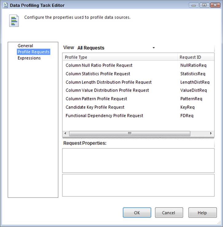
FIGURE 12-5
10.Return to the General tab of the editor. In the Destination property box, choose New File Connection. This is where you will select the location of the XML file where the Data Profiling Task stores its profile output when it is run.
11.In the File Connection Manager Editor, change the Usage type dropdown to “Create file” and enter C:\ProSSIS\Data\Employee_Profile.xml in the File text box. Click OK to save your changes to the connection, and click OK again to save your changes in the Data Profiling Task Editor.
12.Now it is time to execute this simple package. Run the package in Visual Studio, which will initiate several queries against the source table or view (in this case, a view). Because this view returns only a few rows, the Data Profiling task will execute rather quickly, but with large tables it may take several minutes (or longer if your table has millions of rows and you are performing several profiling tests at once).
The results of the profile are stored in the Employee_Profile.xml file, which you will next review with the Data Profile Viewer tool.
Reviewing the Results of the Data Profiling Task
Despite common user expectations, data cannot be magically generated, no matter how creative you are with data cleansing. For example, suppose you are building a sales target analysis that uses employee data, and you are asked to build into the analysis a sales territory group, but the source column has only 50 percent of the data populated. In this case, the business user needs to rethink the value of the data or fix the source. This is a simple example for the purpose of the tutorials in this chapter, but consider a more complicated example or a larger table.
The point is that your source data is likely to be of varying quality. Some data is simply missing, other data has typos, sometimes a column has so many different discrete values that it is hard to analyze, and so on. The purpose of doing data profiling is to understand the source, for two reasons. First, it enables you to review the data with the business user, which can effect changes; second, it provides the insight you need when developing your ETL operations. In fact, even though we’re bringing together business data that the project stakeholders use every day, we’re going to be using that data in ways that it has never been used before. Because of this, we’re going to learn things about it that no one knows — not even the people who are the domain experts. Data profiling is one of the up-front tasks that helps the project team avoid unpleasant (and costly) surprises later on.
Now that you have run the Data Profiling Task, your next objective is to evaluate the results:
1. Observing the output requires using the Data Profile Viewer. This utility is found in the Integration Services subdirectory for Microsoft SQL Server 2014 (Start Button ⇒ All Programs ⇒ Microsoft SQL Server 2014 ⇒Integration Services) or in Windows 8, simply type Data Profile Viewer at the start screen.
2. Open the Employee_Profile.xml file created earlier by clicking the Open button and navigating to the C:\ProSSIS\Data folder (or the location where the file was saved), highlighting the file, and clicking Open again.
3. In the Profiles navigation tree, first click the table icon on the top left to put the tree viewer into Column View. Then drill down into the details by expanding Data Sources, server (local), Databases, AdventureWorks, and the [Sales].[vSalesPerson] table, as shown in Figure 12-6.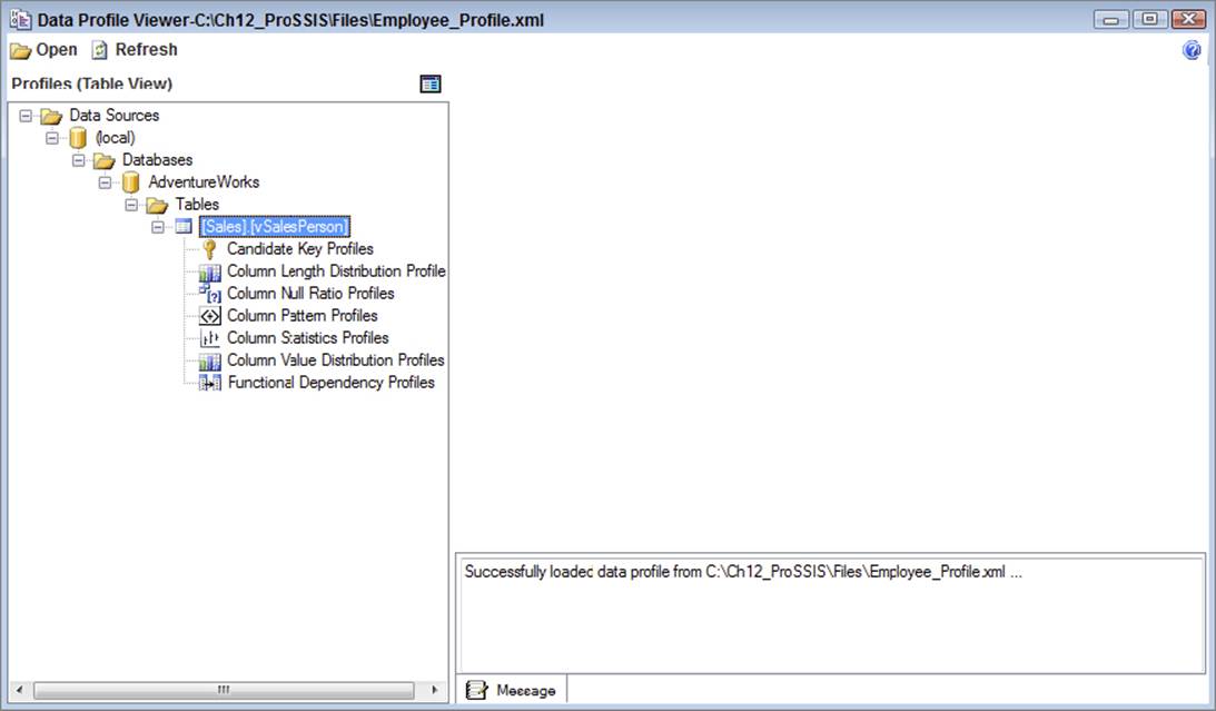
FIGURE 12-6
4. The first profiling output to observe is the Candidate Key Profiles, so click this item under the Columns list, which will open the results in the viewer on the right. Note that the Data Profiling Task has identified seven columns that are unique across the entire table (with 100 percent uniqueness), as shown in Figure 12-7.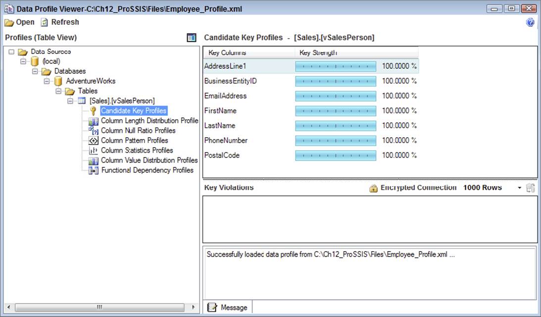
FIGURE 12-7
Given the small size of this table, all these columns are unique, but with larger tables, you will see fewer columns and less than 100 percent uniqueness, and any exceptions or key violations. The question is, which column looks to be the right candidate key for this table? In the next section you will see how this answer affects your ETL.
5. Click the Functional Dependency Profile object on the left and observe the results. This shows the relationship between values in multiple columns. Two columns are shown: Determinant Column(s) and Dependant Column. The question is, for every unique value (or combination) in the Determinant Column, is there only one unique value in the Dependant Column? Observe the output. What is the relationship between these combinations of columns: TerritoryGroup and TerritoryName, StateProvinceName, and CountryRegionName. Again, in the next section you will see how these results affect your ETL.
6. In the profile tree, click the “View Single Column by Profile” icon at the top right of the profile tree. Next, expand the TerritoryName column and highlight the Column Length Distribution. Then, in the distribution profile on the right, double-click the length distribution of 6, as shown in Figure 12-8.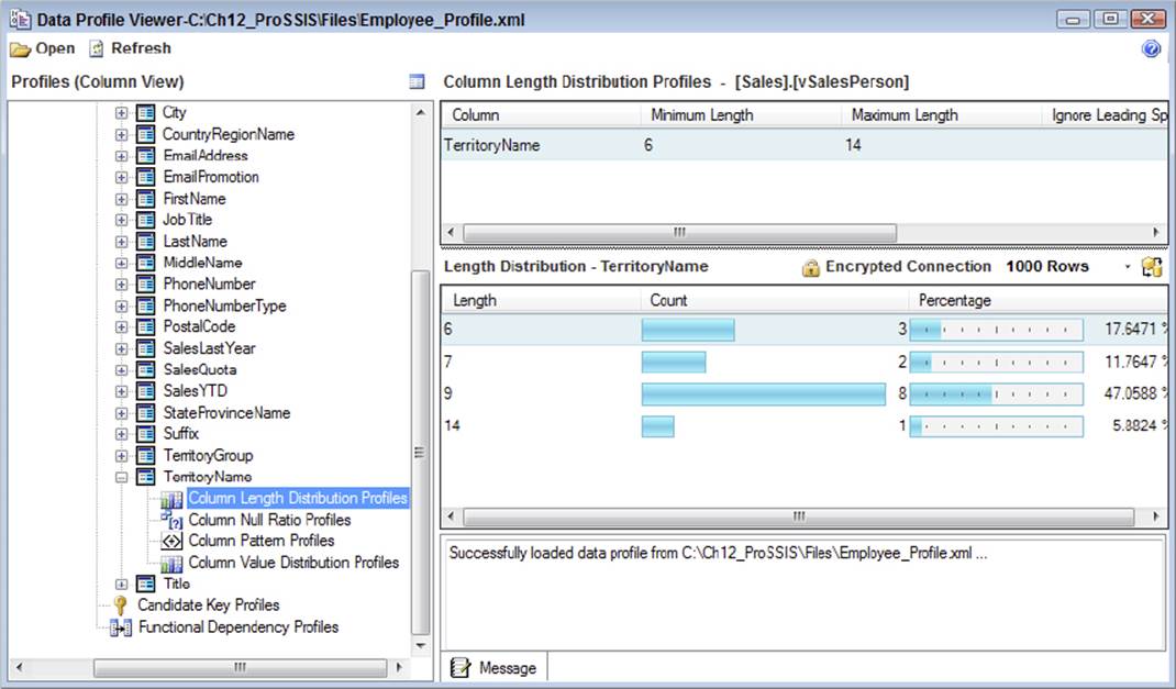
FIGURE 12-8
The column length distribution shows the number of rows by length. What are the maximum and minimum lengths of values for the column?
7. Under TerritoryName in the profile browser, select the Column Null Ratio Profile and then double-click the row in the profile viewer on the right to view the detail rows.
The Column Null Ratio shows what percentage of rows in the entire table have NULL values. This is valuable for ETL considerations because it spells out when NULL handling is required for the ETL process, which is one of the most common transformation processes.
8. Select the Column Value Distribution Profile on the left under the TerritoryName and observe the output in the results viewer. How many unique values are there in the entire table? How many values are used only one time in the table?
9. In the left navigation pane, expand the PhoneNumber column and then click the Column Pattern Profile. Double-click the first pattern, number 1, in the list on the right, as shown in Figure 12-9. As you can see, the bottom right of the window shows the actual data values for the phone numbers matching the selected pattern. This data browser is helpful in seeing the actual values so that you can analyze the effectiveness of the Data Profile Task.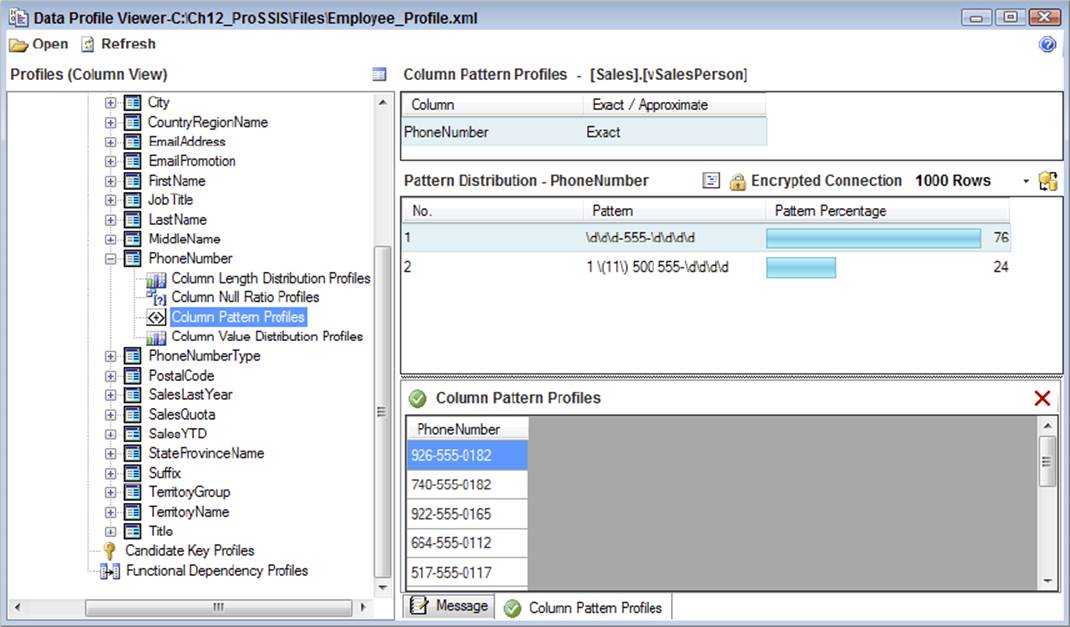
FIGURE 12-9
The Column Pattern Profile uses regular expression syntax to display what pattern or range of patterns the data in the column contains. Notice that for the PhoneNumber column, two patterns emerge. The first is for phone numbers that are in the syntax ###-555-####, which is translated to \d\d\d-555-\d\d\d\d in regular expression syntax. The other pattern begins with 1 \(11\) 500 555- and ends with four variable numbers.
10.The final data profiling type to review is the Column Statistics Profile. This is applicable only to data types related to numbers (integer, float, decimal, numeric) and dates (dates allow only minimum and maximum calculations). In the Profiles tree view on the left of the Data Profile Viewer, expand the SalesYTD column and then click the Column Statistics Profile. Four results are calculated across the spread of values in the numeric column:
a. Minimum: The lowest number value in the set of column values
b. Maximum: The highest number value in the set of column values
c. Mean: The average of values in the set of column values
d. Standard Deviation: The average variance between the values and the mean
The Column Statistics Profile is very valuable for fact table source evaluation, as the measures in a fact table are almost always numeric based, with a few exceptions.
Overall, the output of the Data Profiling Task has helped to identify the quality and range of values in the source. This naturally leads to using the output results to formulate the ETL design.
Turning Data Profile Results into Actionable ETL Steps
The typical first step in evaluating source data is to check the existence of source key columns and referential completeness between source tables or files. Two of the data profiling outputs can help in this effort:
· The Candidate Key Profile will provide the columns (or combination of columns) with the highest uniqueness. It is crucial to identify a candidate key (or composite key) that is 100 percent unique, because when you load your dimension and fact tables, you need to know how to identify a new or existing source record. In the preceding example, shown in Figure 12-7, several columns meet the criteria. The natural selection from this list is the BusinessEntityID column.
· The Column NULL Ratio is another important output of the Data Profiling Task. This can be used to verify that foreign keys in the source table have completeness, especially if the primary key to foreign key relationships will be used to relate a dimension table to a fact, or a dimension table to another dimension table. Of course, this doesn’t verify that the primary-to-foreign key values line up, but it will give you an initial understanding of referential data completeness.
As just mentioned, the Column NULL Ratio can be used for an initial review of foreign keys in source tables or files that have been loaded into SQL Server for data profiling review. The Column NULL Ratio is an excellent output, because it can be used for almost every destination column type, such as dimension attributes, keys, and measures. Anytime you have a column that has NULLs, you will most likely have to replace them with unknowns or perform some data cleansing to handle them.
In Step 7 of the previous section, the Territory Name has approximately a 17 percent NULL ratio. In your dimension model destination this is a problem, because the Employee dimension has a foreign surrogate key to the Sales Territory dimension. Because there isn’t completeness in the SalesTerritory, you don’t have a reference to the dimension. This is an actionable item that you will need to address in the dimension ETL section later.
Other useful output of the Data Profiling Task includes the column length and statistics presented. Data type optimization is important to define; when you have a large inefficient source column where most of the space is not used (such as a char(1000)), you will want to scale back the data type to a reasonable length. To do so, use the Column Length Distribution (refer to Figure 12-8).
The column statistics can be helpful in defining the data type of your measures. Optimization of data types in fact tables is more important than dimensions, so consider the source column’s max and min values to determine what data type to use for your measure. The wider a fact table, the slower it will perform, because fewer rows will fit in the server’s memory for query execution, and the more disk space it will occupy on the server.
Once you have evaluated your source data, the next step is to develop your data extraction, the “E” of ETL.
DATA EXTRACTION AND CLEANSING
Data extraction and cleansing applies to many types of ETL, beyond just data warehouse and BI data processing. In fact, several chapters in this book deal with data extraction for various needs, such as incremental extraction, change data capture, and dealing with various sources. Refer to the following chapters to plan your SSIS data extraction components:
· Chapter 4 takes an initial look at the Source components in the Data Flow that will be used for your extraction.
· Chapter 10 considers data cleansing, which is a common task for any data warehouse solution.
· Chapter 13 deals with using the SQL Server relational engine to perform change data capture.
· Chapter 14 is a look at heterogeneous, or non-SQL Server, sources for data extraction.
The balance of this chapter deals with the core of data warehouse ETL, which is dimension and fact table loading, SSAS object processing, and ETL coordination.
DIMENSION TABLE LOADING
Dimension transformation and loading is about tracking the current and sometime history of associated attributes in a dimension table. Figure 12-10 shows the dimensions related to the Sales Quota Fact table in the AdventureWorksDW database (named FactSalesQuota). The objective of this section is to process data from the source tables into the dimension tables.
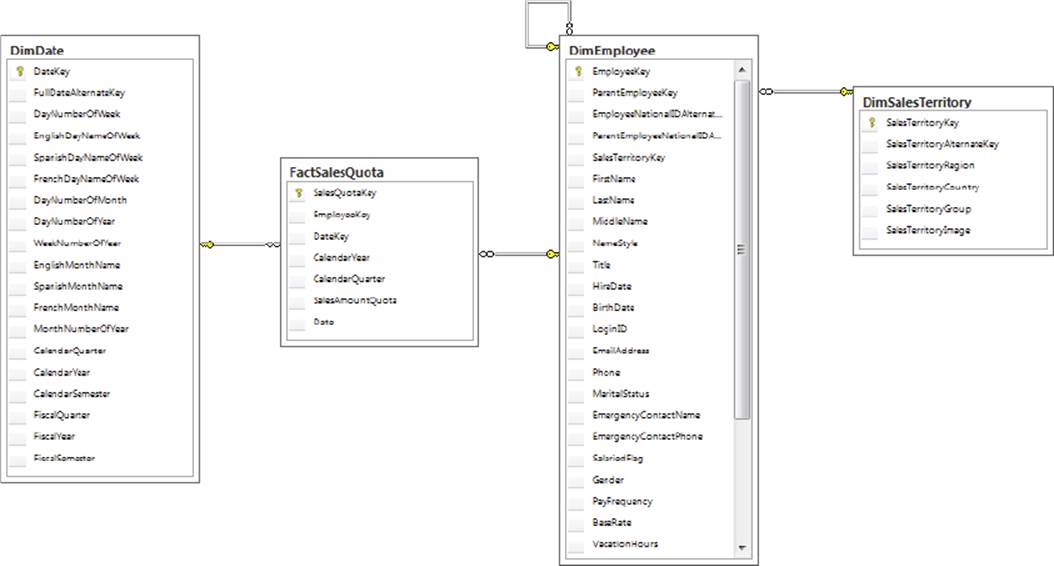
FIGURE 12-10
In this example, notice that each dimension (DimEmployee, DimSalesTerritory, and DimDate) has a surrogate key named Dimension Key, as well as a candidate key named Dimension AlternateKey. The surrogate key is the most important concept in data warehousing because it enables the tracking of change history and optimizes the structures for performance. See The Data Warehouse Toolkit, Third Edition, by Ralph Kimball and Margy Ross (Wiley, 2013), for a detailed review of the use and purpose of surrogate keys. Surrogate keys are often auto-incrementing identity columns that are contained in the dimension table.
Dimension ETL has several objectives, each of which is reviewed in the tutorial steps to load the DimSalesTerritory and DimEmployee tables, including the following:
· Identifying the source keys that uniquely identify a source record and that will map to the alternate key
· Performing any Data Transformations to align the source data to the dimension structures
· Handling the different change types for each source column and adding or updating dimension records
SSIS includes a built-in transformation called the Slowly Changing Dimension (SCD) Transformation to assist in the process. This is not the only transformation that you can use to load a dimension table, but you will use it in these tutorial steps to accomplish dimension loading. The SCD Transformation also has some drawbacks, which are reviewed at the end of this section.
Loading a Simple Dimension Table
Many dimension tables are like the Sales Territory dimension in that they contain only a few columns, and history tracking is not required for any of the attributes. In this example, the DimSalesTerritory table is sourced from the [Sales].[SalesTerritory] table, and any source changes to any of the three columns will be updated in the dimension table. These columns are referred to as changing dimension attributes, because the values can change.
1. To begin creating the ETL for the DimSalesTerritory table, return to your SSIS project created in the first tutorial and create a new package named ETL_DimSalesTerritory.dtsx.
2. Because you will be extracting data from the AdventureWorks database and loading data into the AdventureWorksDW database, create two OLE DB project connections to these databases named AdventureWorks and AdventureWorksDW, respectively. Refer to Chapter 2 for help about defining the project connections.
3. Drag a new Data Flow Task from the SSIS Toolbox onto the Control Flow and navigate to the Data Flow designer.
4. Drag an OLE DB Source component into the Data Flow and double-click the new source to open the editor. Configure the OLE DB Connection Manager dropdown to use the Adventure Works database and leave the data access mode selection as “Table or view.” In the “Name of the table or the view” dropdown, choose [Sales].[SalesTerritory], as shown in Figure 12-11.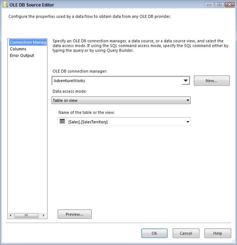
FIGURE 12-11
5. On the Columns property page (see Figure 12-12), change the Output Column value for the TerritoryID column to SalesTerritoryAlternateKey, change the Name column to SalesTerritoryRegion, and change the Output Column for the Group column to SalesTerritoryGroup. Also, uncheck all the columns under SalesTerritoryGroup because they are not needed for the DimSalesTerritory table.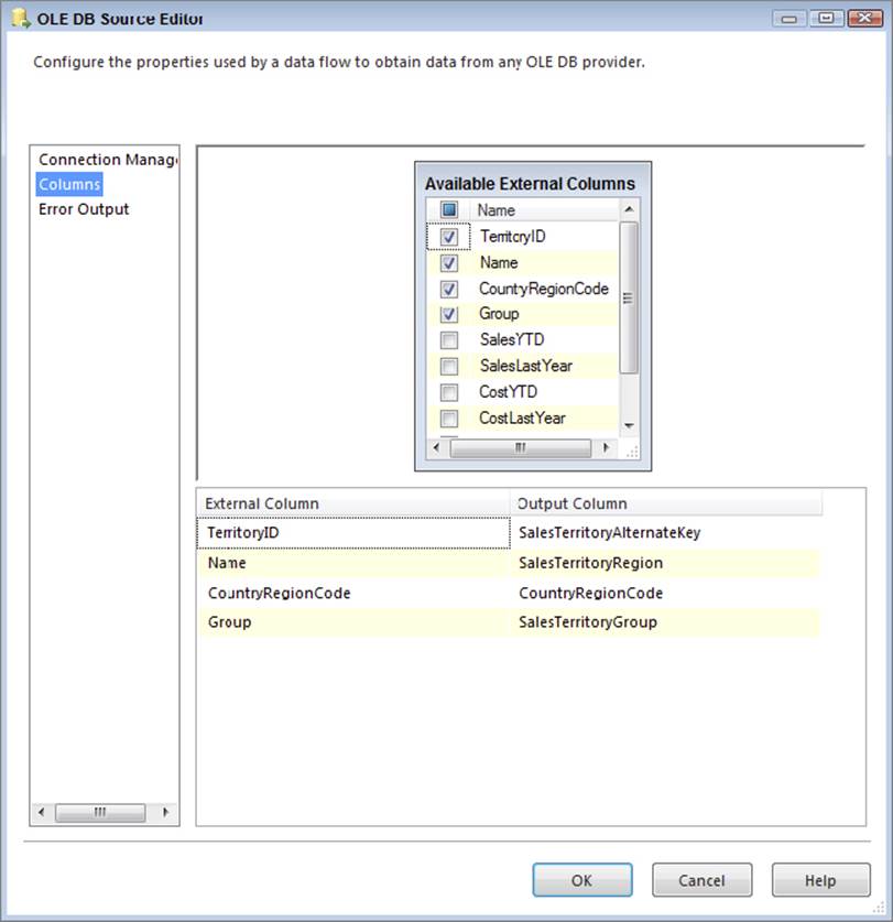
FIGURE 12-12
6. Click OK to save your changes and then drag a Lookup Transformation onto the Data Flow and connect the blue data path from the OLE DB Source onto the Lookup.
7. On the General property page, shown in Figure 12-13, edit the Lookup Transformation as follows: leave the Cache mode setting at Full cache, and leave the Connection type setting at OLE DB Connection Manager.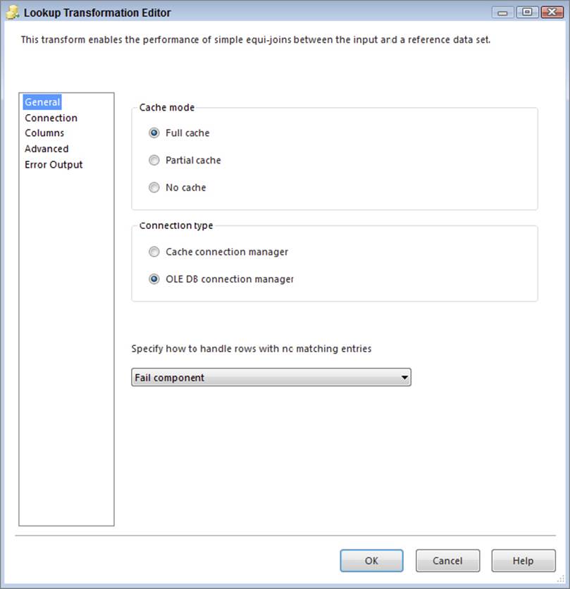
FIGURE 12-13
8. On the Connection property page, set the OLE DB Connection Manager dropdown to the AdventureWorks connection. Change the “Use a table or a view” dropdown to [Person].[CountryRegion].
9. On the Columns property page, drag the CountryRegionCode from the available Input Columns list to the matching column in the Available Lookup Columns list, then select the checkbox next to the Name column in the same column list. Rename the Output Alias of the Name column to SalesTerritoryCountry, as shown in Figure 12-14.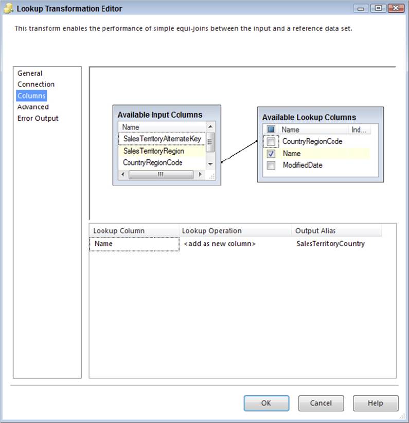
FIGURE 12-14
10.Select OK in the Lookup Transformation Editor to save your changes.
At this point in the process, you have performed some simple initial steps to align the source data up with the destination dimension table. The next steps are the core of the dimension processing and use the SCD Transformation.
11.Drag a Slowly Changing Dimension Transformation from the SSIS Toolbox onto the Data Flow and connect the blue data path output from the Lookup onto the Slowly Changing Dimension Transformation. When you drop the path onto the SCD Transformation, you will be prompted to select the output of the Lookup. Choose Lookup Match Output from the dropdown and then click OK.
12.To invoke the SCD wizard, double-click the transformation, which will open up a splash screen for the wizard. Proceed to the second screen by clicking Next.
13.The first input of the wizard requires identifying the dimension table to which the source data relates. Therefore, choose AdventureWorksDW as the Connection Manager and then choose [dbo].[DimSalesTerritory] as the table or view, which will automatically display the dimension table’s columns in the list, as shown in Figure 12-15. For the SalesTerritoryAlternateKey, change the Key Type to Business key. Two purposes are served here: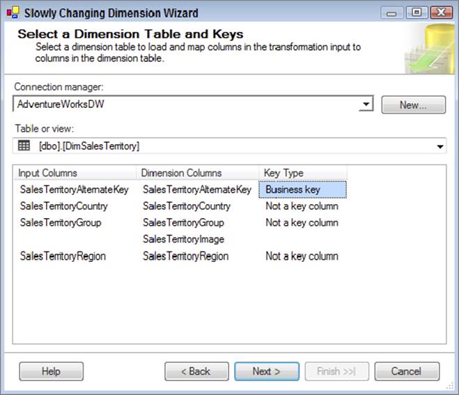
FIGURE 12-15
· One, you identify the candidate key (or business key) from the dimension table and which input column it matches. This will be used to identify row matches between the source and the destination.
· Two, columns are matched from the source to attributes in the dimension table, which will be used on the next screen of the wizard to identify the change tracking type. Notice that the columns are automatically matched between the source input and the destination dimension because they have the same name and data type. In other scenarios, you may have to manually perform the match.
14.On the next screen of the SCD wizard, you need to identify what type of change each matching column is identified as. It has already been mentioned that all the columns are changing attributes for the DimSalesTerritory dimension; therefore, select all the columns and choose the “Changing attribute” Change Type from the dropdown lists, as shown in Figure 12-16.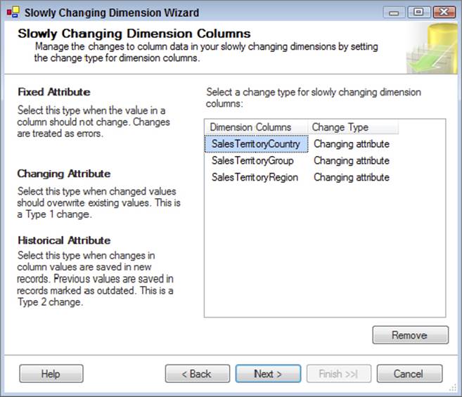
FIGURE 12-16
Three options exist for the Change Type: Changing attribute, Historical attribute, and Fixed attribute. As mentioned earlier, a Changing attribute is updated if the source value changes. For the Historical attribute, when a change occurs, a new record is generated, and the old record preserves the history of the change. You’ll learn more about this when you walk through the DimEmployee dimension ETL in the next section of this chapter. Finally, a Fixed attribute means no changes should happen, and the ETL should either ignore the change or break.
15.The next screen, titled “Fixed and Changing Attribute Options,” prompts you to choose which records you want to update when a source value changes. The “Fixed attributes” option is grayed out because no Fixed attributes were selected on the prior screen. Under the “Changing attributes” option, you can choose to update the changing attribute column for all the records that match the same candidate key, or you can choose to update only the most recent one. It doesn’t matter in this case because there will be only one record per candidate key value, as there are no Historical attributes that would cause a new record. Leave this box unchecked and proceed to the next screen.
16.The “Inferred Dimension Members” screen is about handling placeholder records that were added during the fact table load, because a dimension member didn’t exist when the fact load was run. Inferred members are covered in the DimEmployee dimension ETL, later in this chapter.
17.Given the simplicity of the Sales Territory dimension, this concludes the wizard, and on the last screen you merely confirm the settings that you configured. Select Finish to complete the wizard.
The net result of the SCD wizard is that it will automatically generate several downstream transformations, preconfigured to handle the change types based on the candidate keys you selected. Figure 12-17 shows the completed Data Flow with the SCD Transformation.
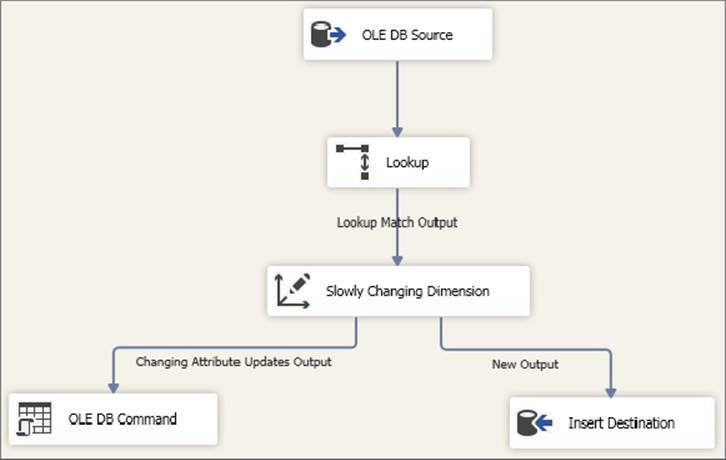
FIGURE 12-17
Since this dimension is simple, there are only two outputs. One output is called New Output, which will insert new dimension records if the candidate key identified from the source does not have a match in the dimension. The second output, called Changing Attribute Updates Output, is used when you have a match across the candidate keys and one or more of the changing attributes does not match between the source input and the dimension table. This OLE DB command uses an UPDATE statement to perform the operation.
Loading a Complex Dimension Table
Dimension ETL often requires complicated logic that causes the dimension project tasks to take the longest amount of time for design, development, and testing. This is due to change requirements for various attributes within a dimension such as tracking history, updating inferred member records, and so on. Furthermore, with larger or more complicated dimensions, the data preparation tasks often require more logic and transformations before the history is even handled in the dimension table itself.
Preparing the Data
To exemplify a more complicated dimension ETL process, in this section you will create a package for the DimEmployee table. This package will deal with some missing data, as identified earlier in your data profiling research:
1. In the SSIS project, create a new package called ETL_DimEmployee.dtsx. Since you’ve already created project connections for AdventureWorks and AdventureWorksDW, you do not need to add these to the new DimEmployee SSIS package.
2. Create a Data Flow Task and add an OLE DB Source component to the Data Flow.
3. Configure the OLE DB Source component to connect to the AdventureWorks connection and change the data access mode to SQL command. Then enter the following SQL code in the SQL command text window (see Figure 12-18):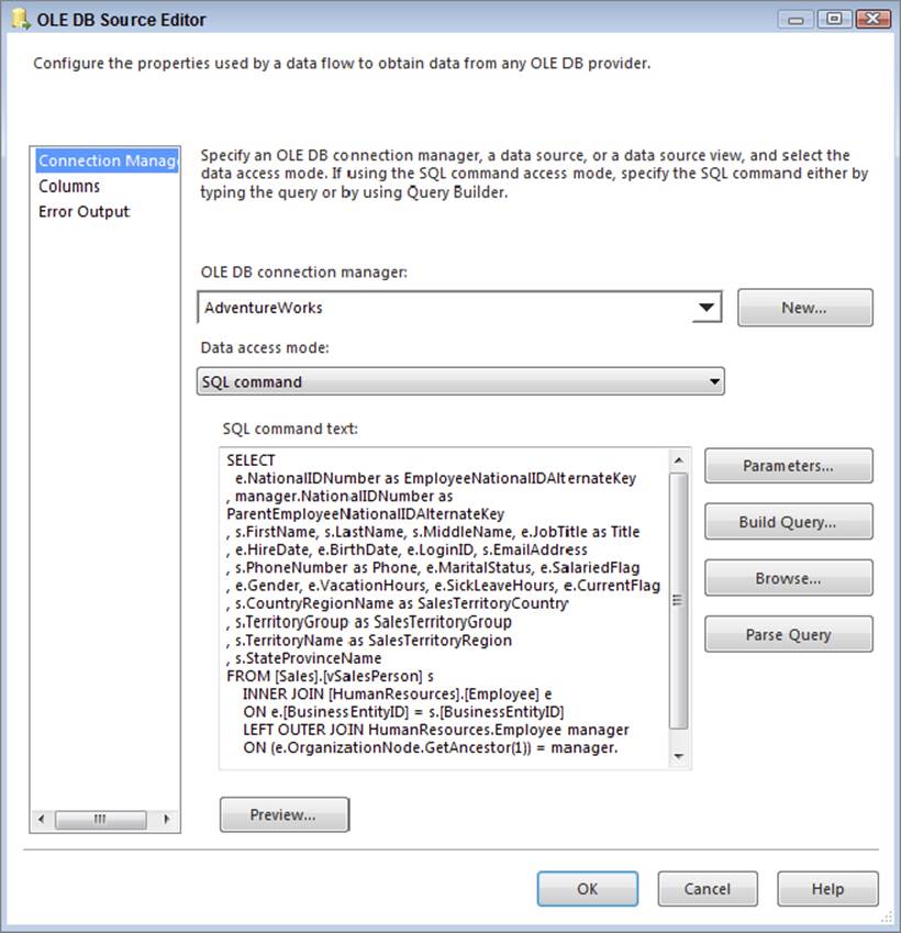
FIGURE 12-18
SELECT
e.NationalIDNumber as EmployeeNationalIDAlternateKey
, manager.NationalIDNumber as ParentEmployeeNationalIDAlternateKey
, s.FirstName, s.LastName, s.MiddleName, e.JobTitle as Title
, e.HireDate, e.BirthDate, e.LoginID, s.EmailAddress
, s.PhoneNumber as Phone, e.MaritalStatus, e.SalariedFlag
, e.Gender, e.VacationHours, e.SickLeaveHours, e.CurrentFlag
, s.CountryRegionName as SalesTerritoryCountry
, s.TerritoryGroup as SalesTerritoryGroup
, s.TerritoryName as SalesTerritoryRegion
, s.StateProvinceName
FROM [Sales].[vSalesPerson] s
INNER JOIN [HumanResources].[Employee] e
ON e.[BusinessEntityID] = s.[BusinessEntityID]
LEFT OUTER JOIN HumanResources.Employee manager
ON (e.OrganizationNode.GetAncestor(1)) = manager.[OrganizationNode]
4. Click OK to save the changes to the OLE DB Source component.
5. Drag a Lookup Transformation to the Data Flow and connect the blue data path output from the OLE DB Source to the Lookup. Name the Lookup Sales Territory.
6. Double-click the Lookup Transformation to bring up the Lookup editor. On the General page, change the dropdown named “Specify how to handle rows with no matching entries” to “Redirect rows to no match output.” Leave the Cache mode as Full cache and the Connection type as OLE DB Connection Manager.
7. On the Connection property page, change the OLE DB connection to AdventureWorksDW and then select [dbo].[DimSalesTerritory] in the dropdown below called “Use a table or a view.”
8. On the Columns property page, join the SalesTerritoryCountry, SalesTerritoryGroup, and SalesTerritoryRegion columns between the input columns and lookup columns, as shown in Figure 12-19. In addition, select the checkbox next to SalesTerritoryKey in the lookup columns to return this column to the Data Flow.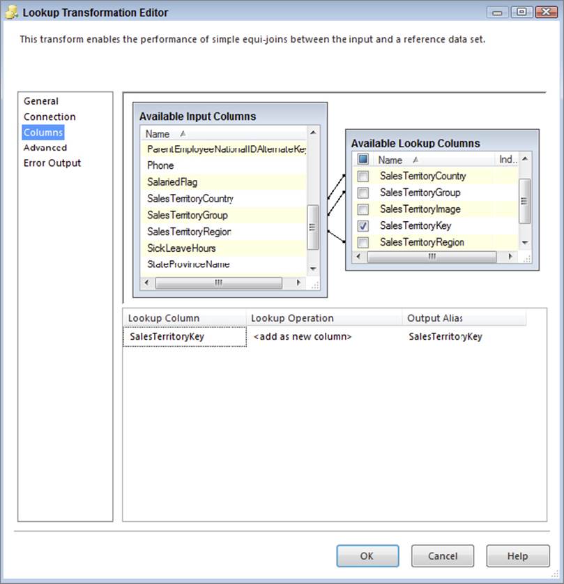
FIGURE 12-19
At this point, recall from your data profiling that some of the sales territory columns in the source have NULL values. Also recall that TerritoryGroup and TerritoryName have a one-to-many functional relationship. In fact, assume that you have conferred with the business users, and they confirmed that you can look at the StateProvinceName and CountryRegionName, and if another salesperson has the same combination of values, you can use their SalesTerritory information.
9. To handle the missing SalesTerritories with the preceding requirements, add a second Lookup Transformation to the Data Flow, and name it Get Missing Territories. Then connect the blue path output of the Sales Territory Lookup to this new Lookup. You will be prompted to choose the Output; select Lookup No Match Output from the dropdown list, as shown in Figure 12-20.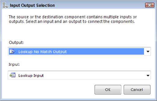
FIGURE 12-20
10.Edit the new Lookup and configure the OLE DB Source component to connect to the AdventureWorks connection. Then change the data access mode to SQL command. Enter the following SQL code in the SQL command text window:
11. SELECT DISTINCT
12. CountryRegionName as SalesTerritoryCountry
13. , TerritoryGroup as SalesTerritoryGroup
14. , TerritoryName as SalesTerritoryRegion
15. , StateProvinceName
16. FROM [Sales].[vSalesPerson]
WHERE TerritoryName IS NOT NULL
17.On the Columns property page, join the SalesTerritoryCountry and StateProvinceName between the input and lookup columns list and then enable the checkboxes next to SalesTerritoryGroup and SalesTerritoryRegion on the lookup list. Append the word “New” to the OutputAlias, as shown in Figure 12-21.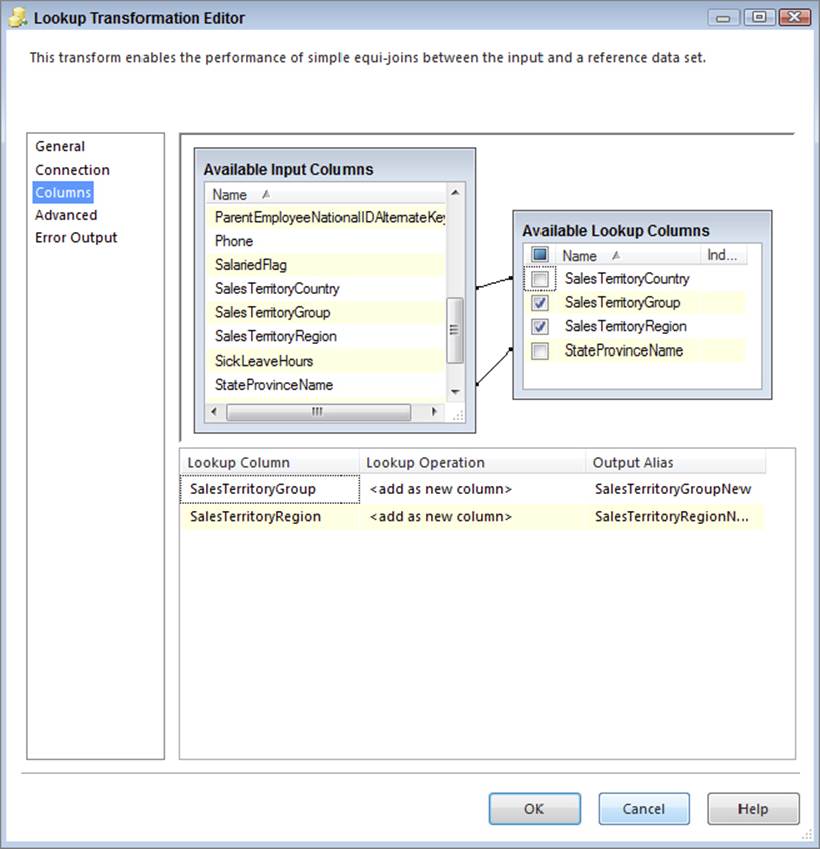
FIGURE 12-21
Next, you will recreate the SalesTerritory Lookup from the prior steps to get the Sales TerritoryKey for the records that originally had missing data.
18.Add a new Lookup to the Data Flow named Reacquire SalesTerritory and connect the output of the Get Missing Territories Lookup (use the Lookup Match Output when prompted). On the General tab, edit the Lookup as follows: leave the Cache mode as Full cache and the Connection type as OLE DB Connection Manager.
19.On the Connections page, specify the AdventureWorksDW Connection Manager and change the “Use a table or a view” option to [dbo].[DimSalesTerritory].
20.On the Columns property page (shown in Figure 12-22), match the columns between the input and lookup table, ensuring that you use the “New” Region and Group column. Match across SalesTerritoryCountry, SalesTerritoryGroupNew, and SalesTerritoryRegionNew. Also return the SalesTerritory Key and name its Output Alias SalesTerritoryKeyNew.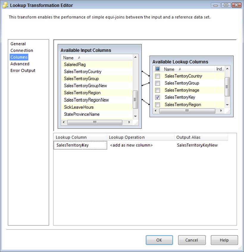
FIGURE 12-22
21.Click OK to save your Lookup changes and then drag a Union All Transformation onto the Data Flow. Connect two inputs into the Union All Transformation:
· The Lookup Match Output from the original Sales Territory Lookup
· The Lookup Match Output from the Reacquire SalesTerritory Lookup (from steps 12–14)
22.Edit the Union All Transformation as follows: locate the SalesTerritoryKey column and change the <ignore> value in the dropdown for the input coming from second lookup to use the SalesTerritoryKeyNew column. This is shown in Figure 12-23.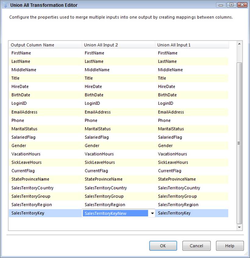
FIGURE 12-23
23.Click OK to save your changes to the Union All. At this point, your Data Flow should look similar to the one pictured in Figure 12-24.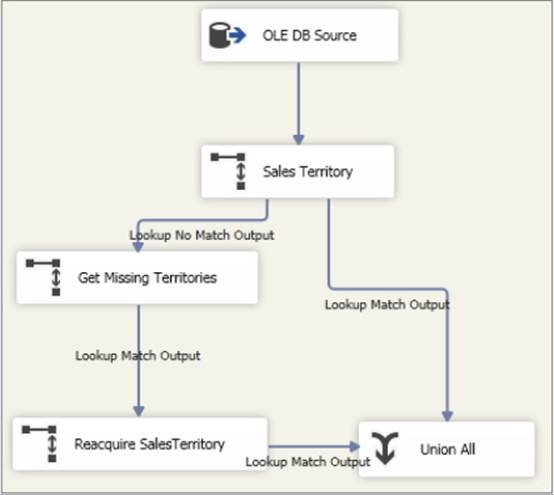
FIGURE 12-24
These steps described how to handle one data preparation task. When you begin to prepare data for your dimension, chances are good you will need to perform several steps to get it ready for the dimension data changes.
You can use many of the other SSIS transformations for this purpose, described in the rest of the book. A couple of examples include using the Derived Column to convert NULLs to Unknowns and the Fuzzy Lookup and Fuzzy Grouping to cleanse dirty data. You can also use the Data Quality Services of SQL Server 2014 to help clean data. A brief overview of DQS is included in Chapter 10.
Handling Complicated Dimension Changes with the SCD Transformation
Now you are ready to use the SCD Wizard again, but for the DimEmployee table, you need to handle different change types and inferred members:
1. Continue development by adding a Slowly Changing Dimension Transformation to the Data Flow and connecting the data path output of the Union All to the SCD Transformation. Then double-click the SCD Transformation to launch the SCD Wizard.
2. On the Select a Dimension Table and Keys page, choose the AdventureWorksDW Connection Manager and the [dbo].[DimEmployee] table.
a. In this example, not all the columns have been extracted from the source, and other destination columns are related to the dimension change management, which are identified in Step 3. Therefore, not all the columns will automatically be matched between the input columns and the dimension columns.
b. Find the EmployeeNationalIDAlternateKey and change the Key Type to Business Key.
c. Select Next.
3. On the Slowly Changing Dimension Columns page, make the following Change Type designations, as shown in Figure 12-25: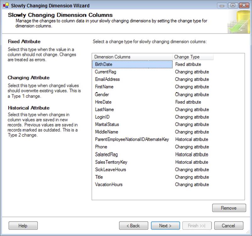
FIGURE 12-25
a. Fixed Attributes: BirthDate, HireDate
b. Changing Attributes: CurrentFlag, EmailAddress, FirstName, Gender, LastName, LoginID, MaritalStatus, MiddleName, Phone, SickLeaveHours, Title, VacationHours
c. Historical Attributes: ParentEmployeeNationalIDAlternateKey, SalariedFlag, SalesTerritoryKey
4. On the Fixed and Changing Attribute Options page, uncheck the checkbox under the Fixed attributes label. The result of this is that when a value changes for a column identified as a fixed attribute, the change will be ignored, and the old value in the dimension will not be updated. If you had checked this box, the package would fail.
5. On the same page, check the box for Changing attributes. As described earlier, this ensures that all the records (current and historical) will be updated when a change happens to a changing attribute.
6. You will now be prompted to configure the Historical Attribute Options, as shown in Figure 12-26. The SCD Transformation needs to know how to identify the current record when a single business key has multiple values (recall that when a historical attribute changes, a new copy of the record is created). Two options are available. One, a single column is used to identify the record. The better option is to use a start and end date. The DimEmployee table has a StartDate and EndDate column; therefore, use the second configuration option button and set the “Start date column” to StartDate, and the “End date column” to EndDate. Finally, set the “Variable to set date values” dropdown to System::StartTime.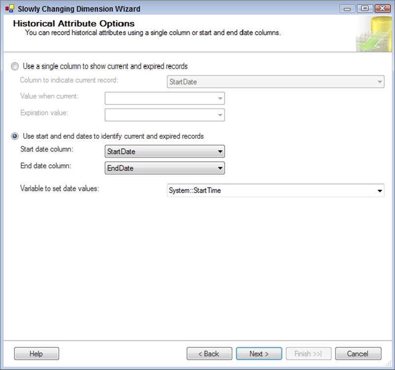
FIGURE 12-26
7. Assume for this example that you may have missing dimension records when processing the fact table. In this case, a new inferred member is added to the dimension. Therefore, on the Inferred Dimension Members page, leave the “Enable inferred member support” option checked. The SCD Transformation needs to know when a dimension member is an inferred member. The best option is to have a column that identifies the record as inferred; however, the DimEmployee table does not have a column for this purpose. Therefore, leave the “All columns with a change type are null” option selected.
8. This concludes the wizard settings. Click Finish so that the SCD Transformation can build the downstream transformations needed based on the configurations. Your Data Flow will now look similar to the one shown in Figure 12-27.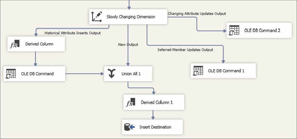
FIGURE 12-27
As you have seen, when dealing with historical attribute changes and inferred members, the output of the SCD Transformation is more complicated with updates, unions, and derived calculations. One of the benefits of the SCD Wizard is rapid development of dimension ETL. Handling changing attributes, new members, historical attributes, inferred members, and fixed attributes is a complicated process that usually takes hours to code, but with the SCD Wizard, you can accomplish this in minutes. Before looking at some drawbacks and alternatives to the SCD Transformation, consider the outputs (refer to Figure 12-27) and how they work:
· Changing Attribute Updates Output: The changing attribute output records are records for which at least one of the attributes that was identified as a changing attribute goes through a change. This update statement is handled by an OLE DB Command Transformation with the code shown here:
·UPDATE [dbo].[DimEmployee]
· SET [CurrentFlag] = ?,[EmailAddress] = ?,[FirstName] = ?,[Gender] =
·?,[LastName] = ?,[LoginID] = ?,[MaritalStatus] = ?,[MiddleName] = ?,
·[Phone] = ?,[SickLeaveHours] = ?,[Title] = ?,[VacationHours] = ?
WHERE [EmployeeNationalIDAlternateKey] = ?
The question marks (?) in the code are mapped to input columns sent down from the SCD Transformation. Note that the last question mark is mapped to the business key, which ensures that all the records are updated. If you had unchecked the changing attribute checkbox in Step 4 of the preceding list, then the current identifier would have been included and only the latest record would have changed.
· New Output: New output records are simply new members that are added to the dimension. If the business key doesn’t exist in the dimension table, then the SCD Transformation will send the row out this output. Eventually these rows are inserted with the Insert Destination (refer to Figure 12-27), which is an OLE DB Destination. The Derived Column 1 Transformation shown in Figure 12-28 is to add the new StartDate of the record, which is required for the metadata management.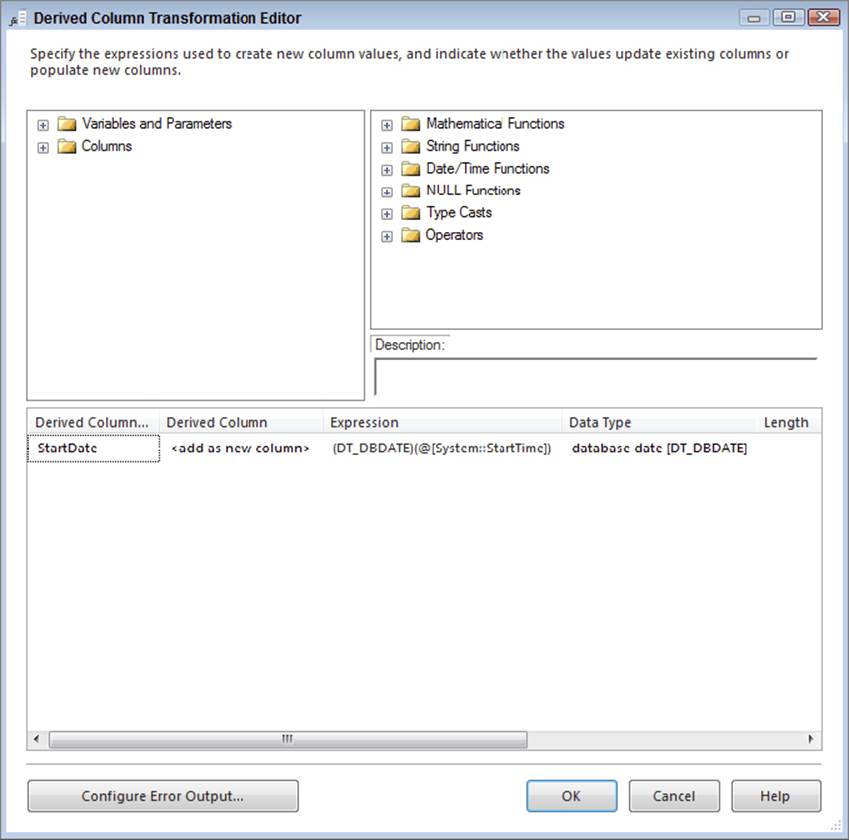
FIGURE 12-28
This dimension is unique, because it has both a StartDate column and a Status column (most dimension tables that track history have either a Status column that indicates whether the record is current or datetime columns that indicate the start and end of the record’s current status, but usually not both). The values for the Status column are Current and <NULL>, so you should add a second Derived Column to this transformation called Status and force a “Current” value in it. You also need to include it in the destination mapping.
· Historical Attribute Inserts Output: The historical output is for any attributes that you marked as historical and underwent a change. Therefore, you need to add a new row to the dimension table. Handling historical changes requires two general steps:
· Update the old record with the EndDate (and NULL Status). This is done through a Derived Column Transformation that defines the EndDate as the System::StartTime variable and an OLE DB command that runs an update statement with the following code:
· UPDATE [dbo].[DimEmployee]
· SET [EndDate] = ?
· , [Status] = NULL
· WHERE [EmployeeNationalIDAlternateKey] = ?
AND [EndDate] IS NULL
· This update statement was altered to also set the Status column to NULL because of the requirement mentioned in the new output. Also, note that [EndDate] IS NULL is included in the WHERE clause because this identifies that the record is the latest record.
· Insert the new version of the dimension record. This is handled by a Union All Transformation to the new outputs. Because both require inserts, this can be handled in one destination. Also note that the Derived Column shown earlier in Figure 12-28 is applicable to the historical output.
· Inferred Member Updates Output: Handling inferred members is done through two parts of the ETL. First, during the fact load when the dimension member is missing, an inferred member is inserted. Second, during the dimension load, if one of the missing inferred members shows up in the dimension source, then the attributes need to be updated in the dimension table. The following update statement is used in the OLE DB Command 1 Transformation:
·UPDATE [dbo].[DimEmployee]
· SET [BirthDate] = ?,[CurrentFlag] = ?,[EmailAddress] = ?,[FirstName] =
·?,[Gender] = ?,[HireDate] = ?,[LastName] = ?,[LoginID] = ?,[MaritalStatus]
·= ?,[MiddleName] = ?,[ParentEmployeeNationalIDAlternateKey] = ?,[Phone] =
·?,[SalariedFlag] = ?,[SalesTerritoryKey] = ?,[SickLeaveHours] = ?, [Title]
·= ?,[VacationHours] = ?
WHERE [EmployeeNationalIDAlternateKey] = ?
What is the difference between this update statement and the update statement used for the changing attribute output? This one includes updates of the changing attributes, the historical attributes, and the fixed attributes. In other words, because you are updating this as an inferred member, all the attributes are updated, not just the changing attributes.
· Fixed Attribute Output (not used by default): Although this is not used by default by the SCD Wizard, it is an additional output that can be used in your Data Flow. For example, you may want to audit records whose fixed attribute has changed. To use it, you can simply take the blue output path from the SCD Transformation and drag it to a Destination component where your fixed attribute records are stored for review. You need to choose the Fixed Attribute Output when prompted by adding the new path.
· Unchanged Output (not used by default): This is another output not used by the SCD Transformation by default. As your dimensions are being processed, chances are good that most of your dimension records will not undergo any changes. Therefore, the records do not need to be sent out for any of the prior outputs. However, you may wish to audit the number of records that are unchanged. You can do this by adding a Row Count Transformation and then dragging a new blue data path from the SCD Transformation onto the Row Count Transformation and choosing the Unchanged Output when prompted by adding the new path. With SSIS in SQL Server 2014, you can also report on the Data Flow performance and statistics when a package is deployed to the SSIS server. Chapter 16 and Chapter 22 review the Data Flow reporting.
Considerations and Alternatives to the SCD Transformation
As you have seen, the SCD Transformation boasts powerful, rapid development, and it is a great tool to understand SCD and ETL concepts. It also helps to simplify and standardize your dimension ETL processing. However, the SCD Transformation is not always the right choice for handling your dimension ETL.
Some of the drawbacks include the following:
· For each row in the input, a new lookup is sent to the relational engine to determine whether changes have occurred. In other words, the dimension table is not cached in memory. That is expensive! If you have tens of thousands of dimension source records or more, the performance of this approach can be a limiting feature of the SCD Transformation.
· For each row in the source that needs to be updated, a new update statement is sent to the dimension table (and updates are used by the changing output, historical output, and inferred member output). If a lot of updates are happening every time your dimension package runs, this will also cause your package to run slowly.
· The Insert Destination is not set to fast load. This is because deadlocks can occur between the updates and the inserts. When the insert runs, each row is added one at a time, which can be very expensive.
· The SCD Transformation works well for historical, changing, and fixed dimension attributes, and, as you saw, changes can be made to the downstream transformations. However, if you open the SCD Wizard again and make a change to any part of it, you will automatically lose your customizations.
Consider some of these approaches to optimize your package that contains the output from the SCD wizard:
· Create an index on your dimension table for the business key, followed by the current row identifier (such as the EndDate). If a clustered index does not already exist, create this index as a clustered index, which will prevent a query plan lookup from getting the underlying row. This will help the lookup that happens in the SCD Transformation, as well as all of the updates.
· The row-by-row updates can be changed to set-based updates. To do this, you need to remove the OLE DB Command Transformation and add a Destination component in its place to stage the records to a temporary table. Then, in the Control Flow, add an Execute SQL Task to perform the set-based update after the Data Flow is completed.
· If you remove all the OLE DB Command Transformations, then you can also change the Insert Destination to use fast load and essentially bulk insert the data, rather than perform per-row inserts.
Overall, these alterations may provide you with enough performance improvements that you can continue to use the SCD Transformation effectively for higher data volumes. However, if you still need an alternate approach, try building the same SCD process through the use of other built-in SSIS transformations such as these:
· The Lookup Transformation and the Merge Join Transformation can be used to cache the dimension table data. This will greatly improve performance because only a single select statement will run against the dimension table, rather than potentially thousands.
· The Derived Column Transformation and the Script component can be used to evaluate which columns have changed, and then the rows can be sent out to multiple outputs. Essentially, this would mimic the change evaluation engine inside of the SCD Transformation.
· After the data is cached and evaluated, you can use the same SCD output structure to handle the changes and inserts, and then you can use set-based updates for better performance.
FACT TABLE LOADING
Fact table loading is often simpler than dimension ETL, because a fact table usually involves just inserts and, occasionally, updates. When dealing with large volumes, you may need to handle partition inserts and deal with updates in a different way.
In general, fact table loading involves a few common tasks:
· Preparing your source data to be at the same granularity as your fact table, including having the dimension business keys and measures in the source data
· Acquiring the dimension surrogate keys for any related dimension
· Identifying new records for the fact table (and potentially updates)
The Sales Quota fact table is relatively straightforward and will give you a good start toward developing your fact table ETL:
1. In your SSIS project for this chapter, create a new package and rename it ETL_FactSalesQuota.dtsx.
2. Just like the other packages you developed in this chapter, you will use two Connection Managers, one for AdventureWorks, and the other for AdventureWorksDW. If you haven’t already created project-level Connection Managers for these in Solution Explorer, add them before continuing.
3. Create a new Data Flow Task and add an OLE DB Source component. Name it Sales Quota Source. Configure the OLE DB Source component to connect to the AdventureWorks Connection Manager, and change the data access mode to SQL command, as shown in Figure 12-29. Add the following code to the SQL command text window: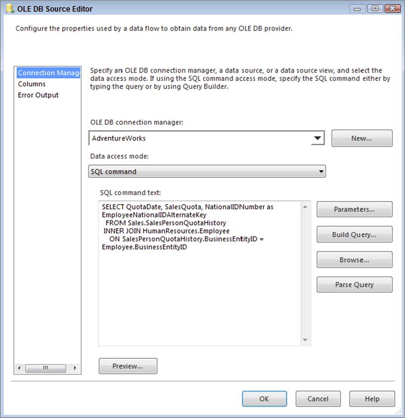
FIGURE 12-29
SELECT QuotaDate, SalesQuota, NationalIDNumber as
EmployeeNationalIDAlternateKey FROM Sales.SalesPersonQuotaHistory
INNER JOIN HumanResources.Employee
ON SalesPersonQuotaHistory.BusinessEntityID = Employee.BusinessEntityID
4. To acquire the surrogate keys from the dimension tables, you will use a Lookup Transformation. Drag a Lookup Transformation onto the Data Flow and connect the blue data path output of the OLE DB Source component onto the Lookup Transformation. Rename the Lookup Employee Key.
5. Double-click the Employee Key Transformation to bring up the Lookup Editor. On the General property page, leave the Cache mode set to Full cache and the Connection type set to OLE DB Connection Manager.
6. On the Connection property page, change the OLE DB Connection Manager dropdown to AdventureWorksDW and enter the following code:
7. SELECT EmployeeKey, EmployeeNationalIDAlternateKey
8. FROM DimEmployee
WHERE EndDate IS NULL
Including the EndDate IS NULL filter ensures that the most current dimension record surrogate key is acquired in the Lookup.
9. Change to the Columns property page and map the EmployeeNationalIDAlternateKey from the input columns to the lookup columns. Then select the checkbox next to the EmployeeKey of the Lookup, as shown in Figure 12-30.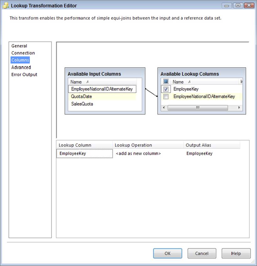
FIGURE 12-30
10.Click OK to save your changes to the Lookup Transformation.
11.For the DateKey, a Lookup is not needed because the DateKey is a “smart key,” meaning the key is an integer value based on the date itself in YYYYMMDD format. Therefore, you will use a Derived column to calculate the DateKey for the fact table. Add a Derived Column Transformation to the Data Flow and connect the blue data path output of the Employee Lookup to the Derived Column Transformation. When prompted, choose the Lookup Match Output from the Lookup Transformation. Name the Derived ColumnDate Keys.
12.Double-click the Derived Column Transformation and add the following three new Derived Column columns and their associated expressions, as shown in Figure 12-31: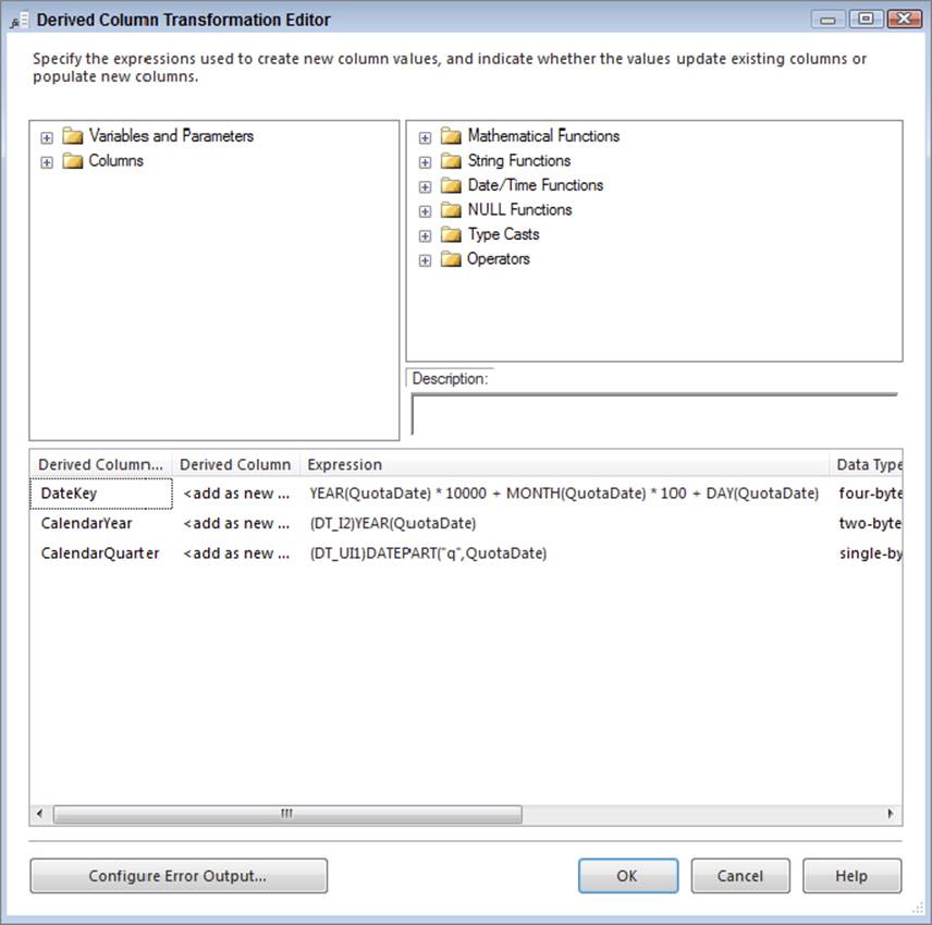
FIGURE 12-31
· DateKey: YEAR([QuotaDate]) *10000 + MONTH([QuotaDate]) *100 + DAY([QuotaDate])
· CalendarYear: (DT_I2) YEAR([QuotaDate])
· CalendarQuarter: (DT_UI1) DATEPART("q",[QuotaDate])
At this point in your Data Flow, the data is ready for the fact table. If your data has already been incrementally extracted, so that you are getting only new rows, you can use an OLE DB Destination to insert it right into the fact table. Assume for this tutorial that you need to identify which records are new and which records are updates, and handle them appropriately. The rest of the steps accomplish fact updates and inserts.
A Merge Join will be used to match source input records to the actual fact table records, but before you add the Merge Join, you need to add a Sort Transformation to the source records (a requirement of the Merge Join) and extract the fact data into the Data Flow.
13.Add a Sort Transformation to the Data Flow and connect the blue data path output from the Derived Column Transformation to the Sort Transformation. Double-click the Sort Transformation to bring up the Sort Transformation Editor and sort the input data by the following columns: EmployeeKey, CalendarYear, and CalendarQuarter, as shown in Figure 12-32. The CalendarYear and CalendarQuarter are important columns for this fact table because they identify the date grain, the level of detail at which the fact table is associated with the date dimension. As a general rule, the Sort Transformation is a very powerful transformation as long as it is working with manageable data sizes, in the thousands and millions, but not the tens or hundreds of millions (if you have a lot of memory, you can scale up as well). An alternate to the Sort is described in steps 12–14, as well as in Chapters 7 and 16.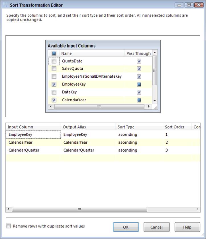
FIGURE 12-32
Figure 12-33 shows what your Data Flow should look like at this point.
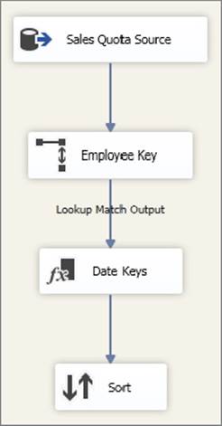
FIGURE 12-33
14.Add a new OLE DB Source component to the Data Flow and name it Sales Quota Fact. Configure the OLE DB Source to use the AdventureWorksDW Connection Manager and use the following SQL command:
15. SELECT EmployeeKey, CalendarYear
16. , CalendarQuarter, SalesAmountQuota
17. FROM dbo.FactSalesQuota
ORDER BY 1,2,3
18.Because you are using an ORDER BY statement in the query (sorting by the first three columns in order), you need to configure the OLE DB Source component to know that the data is entering the Data Flow sorted. First, click OK to save the changes to the OLE DB Source and then right-click the Sales Quota Fact component and choose Show Advanced Editor.
19.On the Input and Output Properties tab, click the OLE DB Source Output object in the left window; in the right window, change the IsSorted property to True, as shown in Figure 12-34.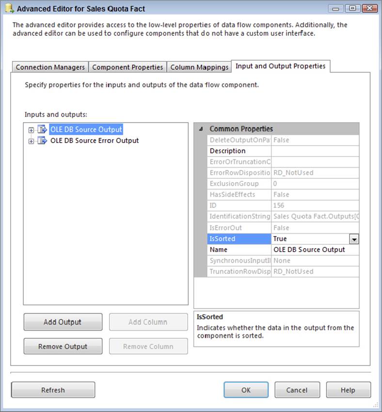
FIGURE 12-34
20.Expand the OLE DB Source Output on the left and then expand the Output Columns folder. Make the following changes to the Output Column properties:
a. Select the EmployeeKey column and change its SortKeyPosition to 1, as shown in Figure 12-35. (If the sort order were descending, you would enter a -1 into the SortKeyPosition.)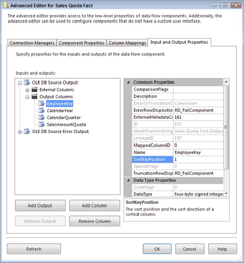
FIGURE 12-35
b. Select the CalendarYear column and change its SortKeyPosition to 2.
c. Select the CalendarQuarter column and change its SortKeyPosition to 3.
d. Click OK to save the changes to the advanced properties.
21.Add a Merge Join Transformation to the Data Flow. First, connect the blue data path output from the Sort Transformation onto the Merge Join. When prompted, choose the input option named Merge Join Left Input. Then connect the blue data path output from the Sales Quota Fact Source to the Merge Join.
22.Double-click the Merge Join Transformation to open its editor. You will see that the EmployeeKey, CalendarYear, and CalendarQuarter columns are already joined between inputs. Make the following changes, as shown in Figure 12-36: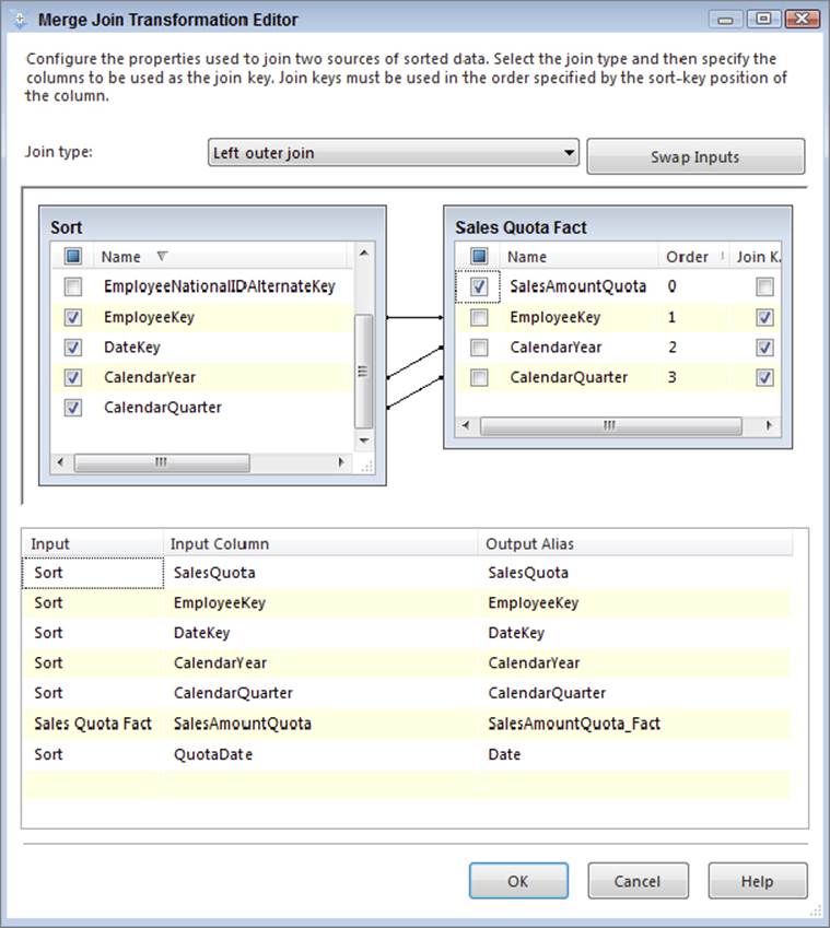
FIGURE 12-36
. Change the Join type dropdown to a Left outer join.
a. Check the SalesQuota, EmployeeKey, DateKey, CalendarYear, CalendarQuarter, and QuotaDate columns from the Sort input list and then change the Output Alias for QuotaDate to Date.
b. Check the SalesAmountQuota from the Sales Quota Fact column list and then change the Output Alias for this column to SalesAmountQuota_Fact.
23.Click OK to save your Merge Join configuration.
24.Your next objective is to identify which records are new quotas and which are changed sales quotas. A conditional split will be used to accomplish this task; therefore, drag a Conditional Split Transformation onto the Data Flow and connect the blue data path output from the Merge Join Transformation to the Conditional Split. Rename the Conditional Split to Identify Inserts and Updates.
25.Double-click the Conditional Split to open the editor and make the following changes, as shown in Figure 12-37: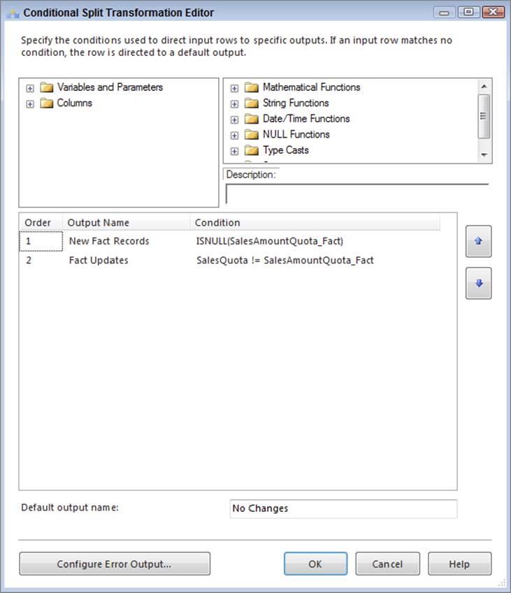
FIGURE 12-37
. Add a new condition named New Fact Records with the following condition: ISNULL([SalesAmountQuota_Fact]). If the measure from the fact is null, it indicates that the fact record does not exist for the employee and date combination.
a. Add a second condition named Fact Updates with the following condition: [SalesQuota] != [SalesAmountQuota_Fact].
b. Change the default output name to No Changes.
26.Click OK to save the changes to the Conditional Split.
27.Add an OLE DB Destination component to the Data Flow and name it Fact Inserts. Drag the blue data path output from the Conditional Split Transformation to the OLE DB Destination. When prompted to choose an output from the Conditional Split, choose the New Fact Records output.
28.Double-click the Fact Inserts Destination and change the OLE DB Connection Manager to AdventureWorksDW. In the “Name of the table or view” dropdown, choose the [dbo].[FactSalesQuota] table.
29.Switch to the Mappings property page and match up the SalesQuota column from the Available Input Columns list to the SalesAmountQuota in the Available Destinations column list, as shown in Figure 12-38. The other columns (EmployeeKey, DateKey, CalendarYear, and CalendarQuarter) should already match. Click OK to save your changes to the OLE DB Destination.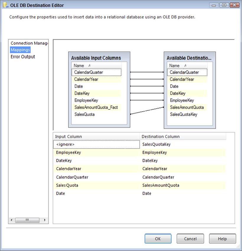
FIGURE 12-38
30.To handle the fact table updates, drag an OLE DB Command Transformation to the Data Flow and rename it Fact Updates. Drag the blue data path output from the Conditional Split onto the Fact Updates Transformation, and when prompted, choose the Fact Update output from the Conditional Split.
31.Double-click the OLE DB Command Transformation and change the Connection Manager dropdown to AdventureWorksDW. On the Component Properties tab, add the following code to the SQLCommand property (make sure you click the ellipsis button to open an editor window):
32. UPDATE dbo.FactSalesQuota
33. SET SalesAmountQuota = ?
34. WHERE EmployeeKey = ?
35. AND CalendarYear = ?
AND CalendarQuarter = ?
36.Switch to the Column Mappings tab and map the SalesQuota to Param_0, Employee_Key to Param_1, CalendarYear to Param_2, and CalendarQuarter to Param_3, as shown in Figure 12-39.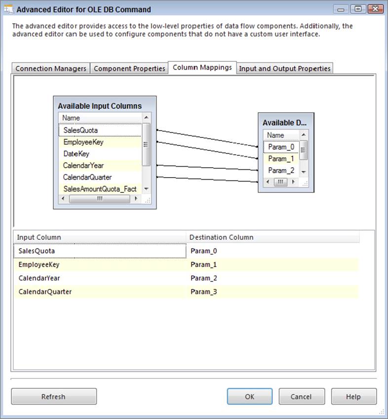
FIGURE 12-39
37.Click OK to save your changes to the OLE DB Command update. Your fact table ETL for the FactSalesQuota is complete and should look similar to Figure 12-40.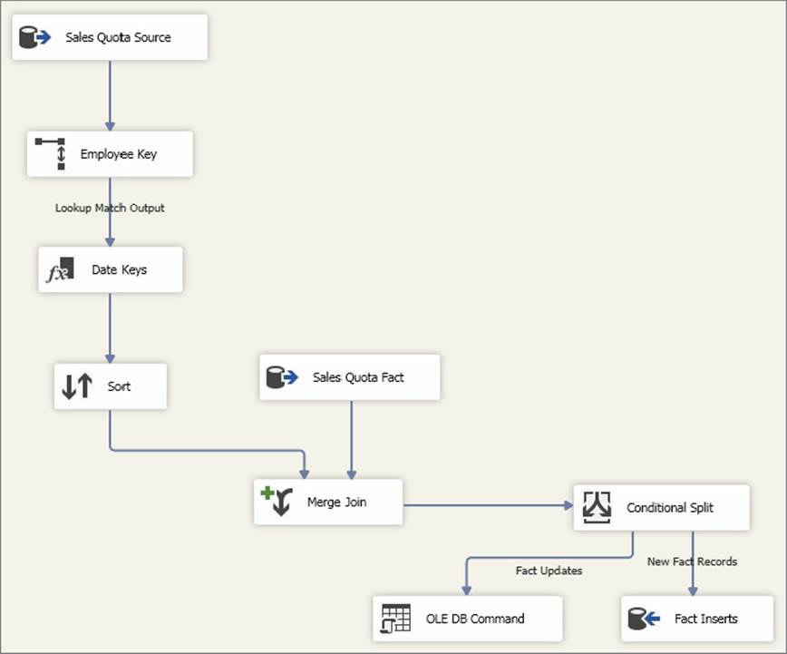
FIGURE 12-40
If you test this package out, you will find that the inserts fail. This is because the date dimension is populated through 2006, but several 2007 and 2008 dates exist that are needed for the fact table. For the purposes of this exercise, you can just drop the foreign key constraint on the table, which will enable your FactSalesQuota package to execute successfully. In reality, as part of your ETL, you would create a recurring script that populated the DateDim table with new dates:
ALTER TABLE [dbo].[FactSalesQuota] DROP CONSTRAINT [FK_FactSalesQuota_DimDate]
Here are some final considerations for fact table ETL:
· A Merge Join was used in this case to help identify which records were updates or inserts, based on matching the source to the fact table. Refer to the Chapter 7 to see other alternatives to associating the source to fact table.
· For the inserts and updates, you may want to leverage the relational engine to handle either the insert or the update at the same time. T-SQL in SQL Server supports a MERGE statement that will perform either an insert or an update depending on whether the record exists. See Chapter 13 for more about how to use this feature.
· Another alternative to the OLE DB Command fact table updates is to use a set-based update. The OLE DB command works well and is easy for small data volumes; however, your situation may not allow per-row updates. Consider staging the updates to a table and then performing a set-based update (through a multirow SQL UPDATE statement) by joining the staging table to the fact table and updating the sales quota that way.
· Inserts are another area of improvement considerations. Fact tables often contain millions of rows, so you should look for ways to optimize the inserts. Consider dropping the indexes, loading the fact table, and then recreating the indexes. This could be much faster. See Chapter 16 for ideas on how to tune the inserts.
· If you have partitions in place, you can insert the data right into the partitioned fact table; however, when you are dealing with high volumes, the relational engine overhead may inhibit performance. In these situations, consider switching the current partition out in order to load it separately, then you can switch it back into the partitioned table.
Inferred members are another challenge for fact table ETL. How do you handle a missing dimension key? One approach includes scanning the fact table source for missing keys and adding the inferred member dimension records before the fact table ETL runs. An alternative is to redirect the missing row when the lookup doesn’t have a match, then add the dimension key during the ETL, followed by bringing the row back into the ETL through a Union All. One final approach is to handle the inferred members after the fact table ETL finishes. You would need to stage the records that have missing keys, add the inferred members, and then reprocess the staged records into the fact table.
As you can see, fact tables have some unique challenges, but overall they can be handled effectively with SSIS. Now that you have loaded both your dimensions and fact tables, the next step is to process your SSAS cubes, if SSAS is part of your data warehouse or business intelligence project.
SSAS PROCESSING
Processing SSAS objects in SSIS can be as easy as using the Analysis Services Processing Task. However, if your SSAS cubes require adding or processing specific partitions or changing the names of cubes or servers, then you will need to consider other approaches. In fact, many, if not most, solutions require using other processing methods.
SSAS in SQL Server 2014 has two types of models, multidimensional and tabular. Both of these models require processing. For multidimensional models, you are processing dimensions and cube partitions. For tabular models, you are processing tables and partitions. However, both models have similar processing options.
The primary ways to process SSAS models through SSIS include the following:
· Analysis Services Processing Task: Can be defined with a unique list of dimensions, tables, and partitions to process. However, this task does not allow modifications of the objects through expressions or configurations.
· Analysis Services Execute DDL Task: Can process objects through XMLA scripts. The advantage of this task is the capability to make the script dynamic by changing the script contents before it is executed.
· Script Task: Can use the API for SSAS, which is called AMO (or Analysis Management Objects). With AMO, you can create objects, copy objects, process objects, and so on.
· Execute Process Task: Can run ascmd.exe, which is the SSAS command-line tool that can run XMLA, MDX, and DMX queries. The advantage of the ascmd.exe tool is the capability to pass in parameters to a script that is run.
To demonstrate the use of some of these approaches, this next tutorial demonstrates processing a multidimensional model using the Analysis Services Processing Task to process the dimensions related to the sales quotas, and then the Analysis Services Execute DDL Task to handle processing of the partitions.
Before beginning these steps, create a new partition in SSAS for the Sales Targets Measure called Sales_Quotas_2014. This is for demonstration purposes. An XMLA script has been created and included in the downloadable content atwww.wrox.com/go/prossis2014 for this chapter called Sales_Quotas_2014.xmla.
1. In your SSIS project for this chapter, create a new package and rename it SSAS_SalesTargets.dtsx.
2. Since this is the only package that will be using the SSAS connection, you will create a package connection, rather than a project connection. Right-click in the Connection Managers window and choose New Analysis Services Connection. In the Add Analysis Services Connection Manager window, click the Edit button to bring up the connection properties, as shown in Figure 12-41.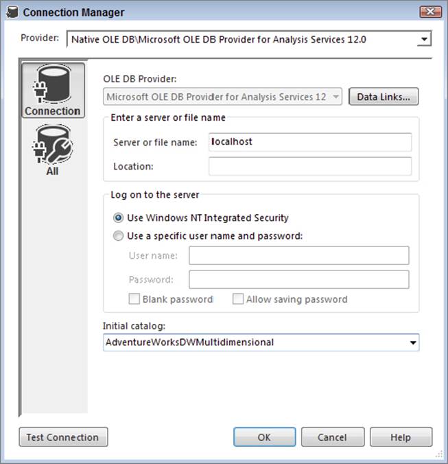
FIGURE 12-41
a. Specify your server in the “Server or file name” text box (such as localhost if you are running SSAS on the same machine).
b. Change the “Log on to the server” option to Use Windows NT Integrated Security.
c. In the Initial catalog dropdown box, choose the Adventure Works SSAS database, which by default is named Adventure Works DW Multidimensional. Please remember that you will need to download and install the sample SSAS cube database, which is available from www.wrox.com/go/prossis2014.
d. Click OK to save your changes to the Connection Manager and then click OK in the Add Analysis Services Connection Manager window.
e. Finally, rename the connection in the SSIS Connection Managers window to AdventureWorksAS.
3. To create the dimension processing, drag an Analysis Services Processing Task from the SSIS Toolbox onto the Control Flow and rename the task Process Dimensions.
4. Double-click the Process Dimensions Task to bring up the editor and navigate to the Processing Settings property page.
a. Confirm that the Analysis Services Connection Manager dropdown is set to AdventureWorksAS.
b. Click the Add button to open the Add Analysis Services Object window. As shown in Figure 12-42, check the Date, Employee, and Sales Territory dimensions and then click OK to save your changes.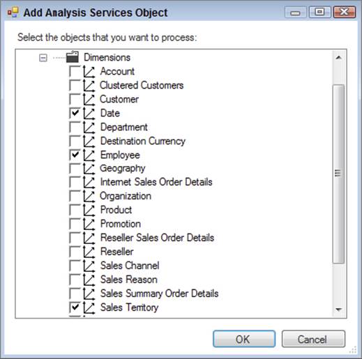
FIGURE 12-42
c. For each dimension, change the Process Options dropdown to Process Default, which will either perform a dimension update or, if the dimension has never been processed, fully process the dimension.
d. Click the Change Settings button, and in the Change Settings editor, click the Parallel selection option under the Processing Order properties. Click OK to save your settings.
e. Click OK to save your changes to the Analysis Services Processing Task.
5. Before continuing, you will create an SSIS package variable that designates the XMLA partition for processing. Name the SSIS variable Sales_Quota_Partition and define the variable with a String data type and a value of “Fact Sales Quota.”
6. Drag an Analysis Services Execute DDL Task onto the Data Flow and drag the green precedence constraint from the Process Dimensions Task onto the Analysis Services Execute DDL Task. Rename the Analysis Services Execute DDL Task Process Partition.
a. Edit the Process Partition Task and navigate to the DDL property page.
b. Change the Connection property to AdventureWorksAS and leave the SourceType as Direct Input, as shown in Figure 12-43.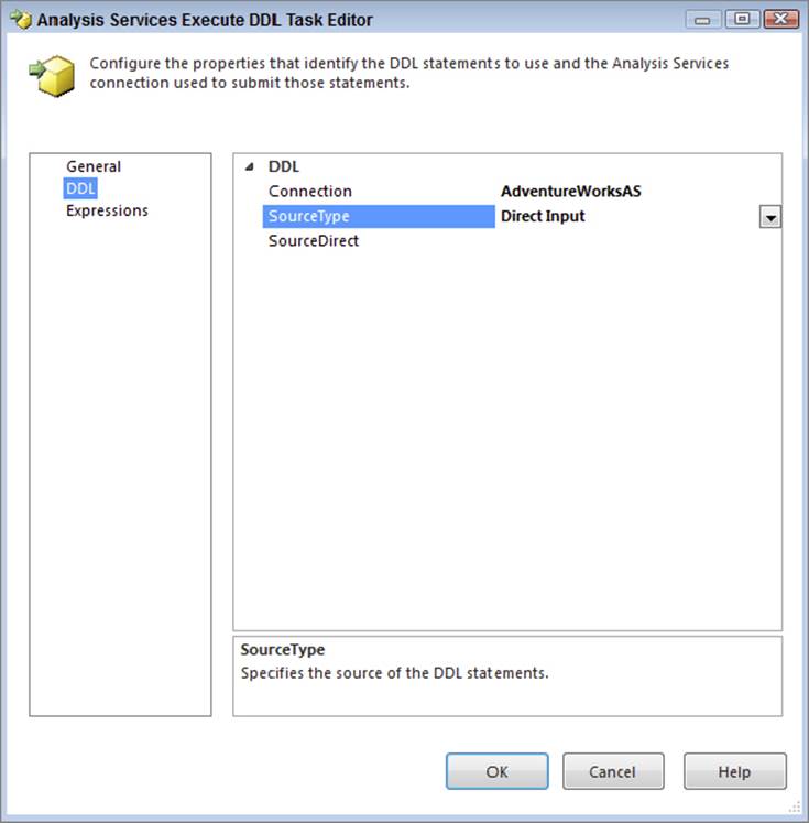
FIGURE 12-43
c. Change to the Expressions property page of the editor and click the Expressions property in the right window. Click the ellipsis on the right side of the text box, which will open the Property Expressions Editor. Choose Source from the dropdown, as shown inFigure 12-44.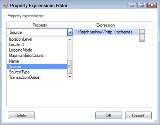
FIGURE 12-44
d. Now you need to add the XMLA code that will execute when the package is run. The expressions will dynamically update the code when this task executes. Click the ellipsis on the right side of the Source property (refer to Figure 12-44) to open Expression Builder.
e. Enter the following code in the Expression text box, which is also shown in Figure 12-45: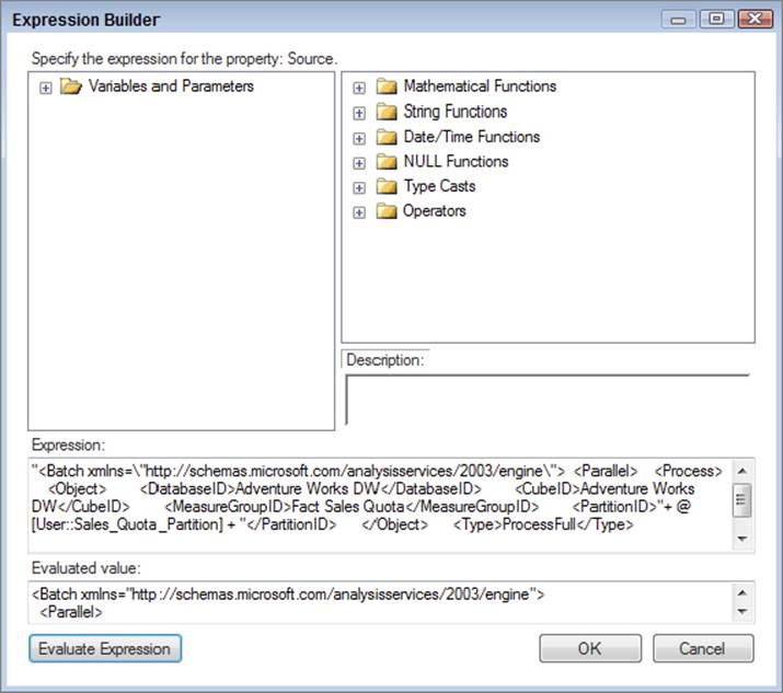
FIGURE 12-45
“<Batch xmlns=\"http://schemas.microsoft.com/analysisservices/2003/engine\">
<Parallel>
<Process>
<Object>
<DatabaseID>Adventure Works DW</DatabaseID>
<CubeID>Adventure Works DW</CubeID>
<MeasureGroupID>Fact Sales Quota</MeasureGroupID>
<PartitionID>"
+ @[User::Sales_Quota_Partition]
+ "</PartitionID>
</Object>
<Type>ProcessFull</Type>
<WriteBackTableCreation>UseExisting</WriteBackTableCreation>
</Process>
</Parallel>
</Batch>"
"
f. This code generates the XMLA and includes the Sales_Quota_Partition variable. The good news is that you don’t need to know XMLA; you can use SSMS to generate it for you.
To automatically generate the XMLA code that will process a Sales Quota partition, open SSMS and connect to SSAS. Expand the Databases folder, then the Adventure Works SSAS database, then the Cubes folder; then expand the Adventure Works cube; and finally expand the Sales Targets measure group. Right-click the Sales Quota 2014 partition and choose Process, as shown in Figure 12-46.
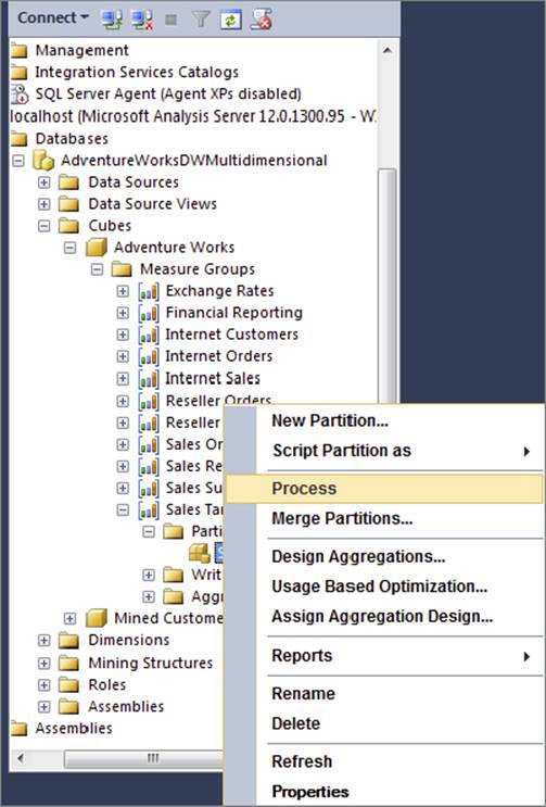
FIGURE 12-46
The processing tool in SSMS looks very similar to the SSAS processing task in SSIS except that the SSMS processing tool has a Script button near the title bar. Click the Script button.
g. Click OK in the open windows to save your changes. The purpose of creating the script and saving the file is to illustrate that you can build your own processing with XMLA and either execute the code in SSMS (clicking on the Execute button) or execute the file through the Analysis Services Execute DDL Task.
7. The SSIS package that you have just developed should look similar to Figure 12-47.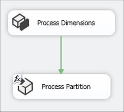
FIGURE 12-47
If you were to fully work out the development of this package, you would likely have a couple more tasks involved in the process. First, the current partition is entered in the variable, but you haven’t yet put the code in place to update this variable when the package is run. For this task, either you could use an Execute SQL Task to pull the value for the current partition from a configuration table or the system date into the variable, or you could use a Script Task to populate the variable.
Second, if you have a larger solution with many partitions that are at the weekly or monthly grain, you would need a task that created a new partition, as needed, before the partition was run. This could be an Analysis Services Execute DDL Task similar to the one you just created for the processing Task, or you could use a Script Task and leverage AMO to create or copy an existing partition to a new partition.
As you have seen, processing SSAS objects in SSIS can require a few simple steps or several more complex steps depending on the processing needs of your SSAS solution.
USING A MASTER ETL PACKAGE
Putting it all together is perhaps the easiest part of the ETL process because it involves simply using SSIS to coordinate the execution of the packages in the required order.
The best practice to do this is to use a master package that executes the child packages, leveraging the Execute Package Task. The determination of precedence is a matter of understanding the overall ETL and the primary-to-foreign key relationships in the tables.
The following steps assume that you are building your solution using the project deployment model. With the project deployment model, you do not need to create connections to the other packages in the project. If you are instead deploying your packages to the file system, you need to create and configure File Connection Managers for each child package, as documented in SQL Server Books Online.
1. Create a new package in your project called Master_ETL.dtsx.
2. Drag an Execute Package Task from the SSIS Toolbox into the Control Flow.
3. Double-click the Execute Package Task to open the task editor.
4. On the Package property page, leave the ReferenceType property set to Project Reference. For the PackageNameFromProjectReference property, choose the ETL_DimSalesTerritory.dtsx package.
Your Execute Package Task will look like the one pictured in Figure 12-48.
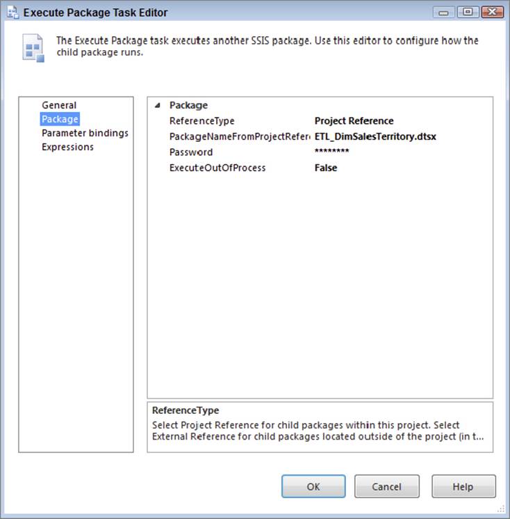
FIGURE 12-48
The ETL packages for the dimension tables are executed, followed by the fact table ETL and concluding with the cube processing. The master package for the examples in this chapter is shown in Figure 12-49.
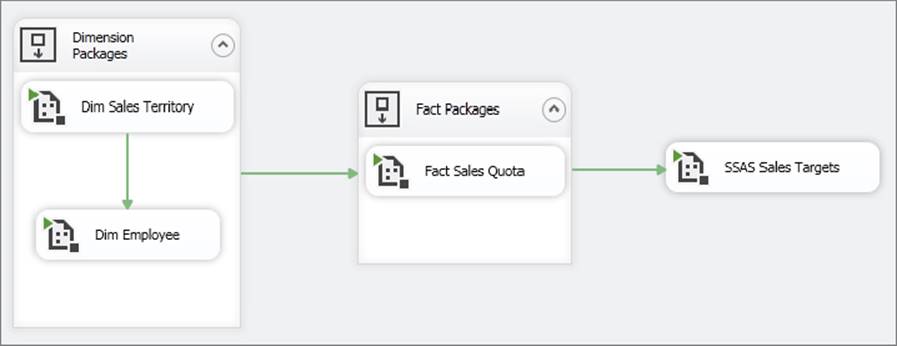
FIGURE 12-49
The related packages are grouped with Sequence containers to help visualize the processing order. In this case, the Dim Sales Territory package needs to be run before the Dim Employee package because of the foreign key reference in the DimEmployee table. Larger solutions will have multiple dimension and fact packages.
SUMMARY
Moving from start to finish in a data warehouse ETL effort requires a lot of planning and research. This research should include both data profiling and interviews with the business users to understand how they will be using the dimension attributes, so that you can identify the different attribute change types.
As you develop your dimension and fact packages, you will need to carefully consider how to most efficiently perform inserts and updates, paying particular attention to data changes and missing members. Finally, don’t leave your SSAS processing packages for the last minute. You may be surprised at the time it can take to develop a flexible package that can dynamically handle selective partition processing and creation.
In the next chapter, you will learn about the pros and cons of using the relational engine instead of SSIS.
All materials on the site are licensed Creative Commons Attribution-Sharealike 3.0 Unported CC BY-SA 3.0 & GNU Free Documentation License (GFDL)
If you are the copyright holder of any material contained on our site and intend to remove it, please contact our site administrator for approval.
© 2016-2026 All site design rights belong to S.Y.A.