Professional Microsoft SQL Server 2014 Integration Services (Wrox Programmer to Programmer), 1st Edition (2014)

Chapter 13. Using the Relational Engine

WHAT’S IN THIS CHAPTER?

· Using the relational engine to facilitate SSIS data extraction

· Loading data with SSIS and the relational engine

· Understanding when to use the relational engine versus SSIS

WROX.COM CODE DOWNLOADS FOR THIS CHAPTER

You can find the wrox.com code downloads for this chapter at http://www.wrox.com/go/prossis2014 on the Download Code tab.

An old adage says that when you’re holding a hammer, everything looks like a nail. When you use SSIS to build a solution, make sure that you use the right tool for each problem you tackle. SSIS will be excellent for some jobs, and SQL Server will shine at other tasks. When used in concert, the combination of the two can be powerful.

This chapter discusses other features in the SQL Server arsenal that can help you build robust and high-performance ETL solutions. The SQL Server relational database engine has many features that were designed with data loading in mind, and as such the engine and SSIS form a perfect marriage to extract, load, and transform your data.

This chapter assumes you are using SQL Server 2014 as the source system, though many of the same principles will apply to earlier versions of SQL Server and to other relational database systems too. You should also have the SQL Server 2014 versions of AdventureWorks and AdventureWorksDW installed; these are available from www.wrox.com.

The easiest way to understand how the relational database engine can help you design ETL solutions is to segment the topic into the three basic stages of ETL: extraction, transformation, and loading. Because the domain of transformation is mostly within SSIS itself, there is not much to say there about the relational database engine, so our scope of interest here is narrowed down to extraction and loading.

DATA EXTRACTION

Even if a data warehouse solution starts off simple — using one or two sources — it can rapidly become more complex when the users begin to realize the value of the solution and request that data from additional business applications be included in the process. More data increases the complexity of the solution, but it also increases the execution time of the ETL. Storage is certainly cheap today, but the size and amount of data are growing exponentially. If you have a fixed batch window of time in which you can load the data, it is essential to minimize the expense of all the operations. This section looks at ways of lowering the cost of extraction and how you can use those methods within SSIS.

SELECT ∗ Is Bad

In an SSIS Data Flow, the OLE DB Source and ADO.NET Source Components allow you to select a table name that you want to load, which makes for a simple development experience but terrible runtime performance. At runtime the component issues a SELECT * FROM «table» command to SQL Server, which obediently returns every single column and row from the table.

This is a problem for several reasons:

· CPU and I/O cost: You typically need only a subset of the columns from the source table, so every extra column you ask for incurs processing overhead in all the subsystems it has to travel through in order to get to the destination. If the database is on a different server, then the layers include NTFS (the file system), the SQL Server storage engine, the query processor, TDS (tabular data stream, SQL Server’s data protocol), TCP/IP, OLE DB, the SSIS Source component, and finally the SSIS pipeline (and probably a few other layers). Therefore, even if you are extracting only one redundant integer column of data from the source, once you multiply that cost by the number of rows and processing overhead, it quickly adds up. Saving just 5 percent on processing time can still help you reach your batch window target.

· Robustness: If the source table has ten columns today and your package requests all the data in a SELECT * manner, then if tomorrow the DBA adds another column to the source table, your package could break. Suddenly the package has an extra column that it doesn’t know what to do with, things could go awry, and your Data Flows will need to be rebuilt.

· Intentional design: For maintenance, security, and self-documentation reasons, the required columns should be explicitly specified.

· DBA 101: If you are still not convinced, find any seasoned DBA, and he or she is likely to launch into a tirade of why SELECT * is the root of all evil.

As Figure 13-1 shows, the Source components also give you the option of using checkboxes to select or deselect the columns that you require, but the problem with this approach is that the filtering occurs on the client-side. In other words, all the columns are brought across (incurring all that I/O overhead), and then the deselected columns are deleted once they get to SSIS.

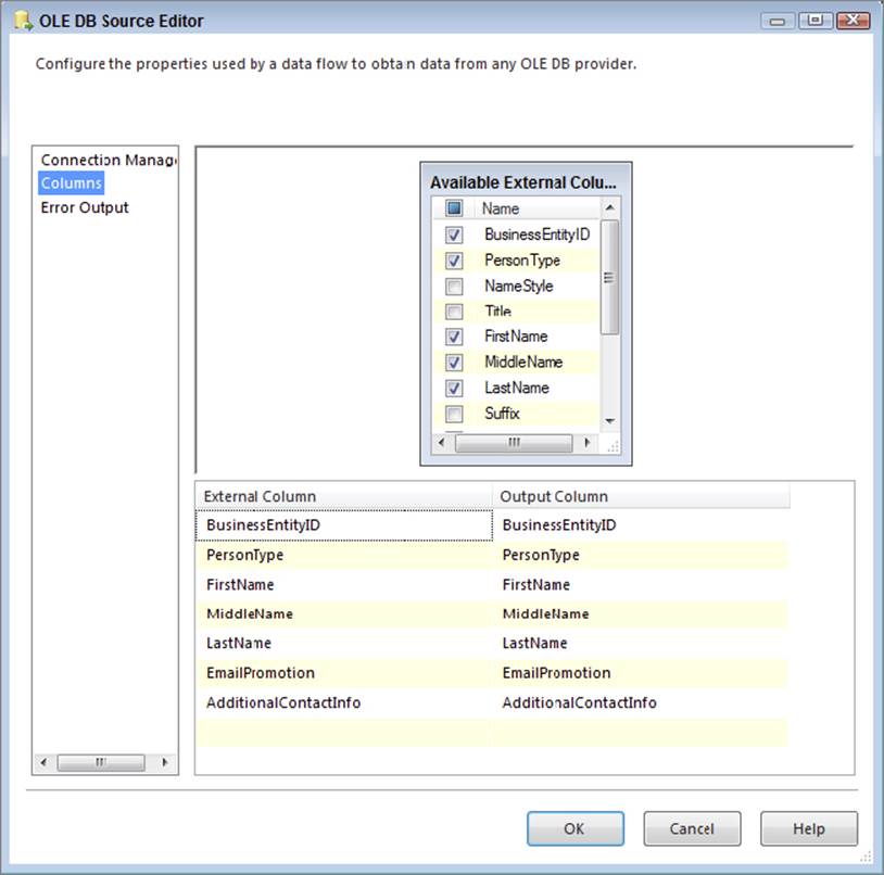
FIGURE 13-1

So what is the preferred way to extract data using these components? The simple answer is to forget that the table option exists and instead use only the query option. In addition, forget that the column checkboxes exist. For rapid development and prototyping these options may be useful, but for deployed solutions you should type in a query to only return the necessary columns. SSIS makes it simple to do this by providing a query builder in both the OLE DB and ADO.NET Source Components, which enables you to construct a query in a visual manner, as shown in Figure 13-2.

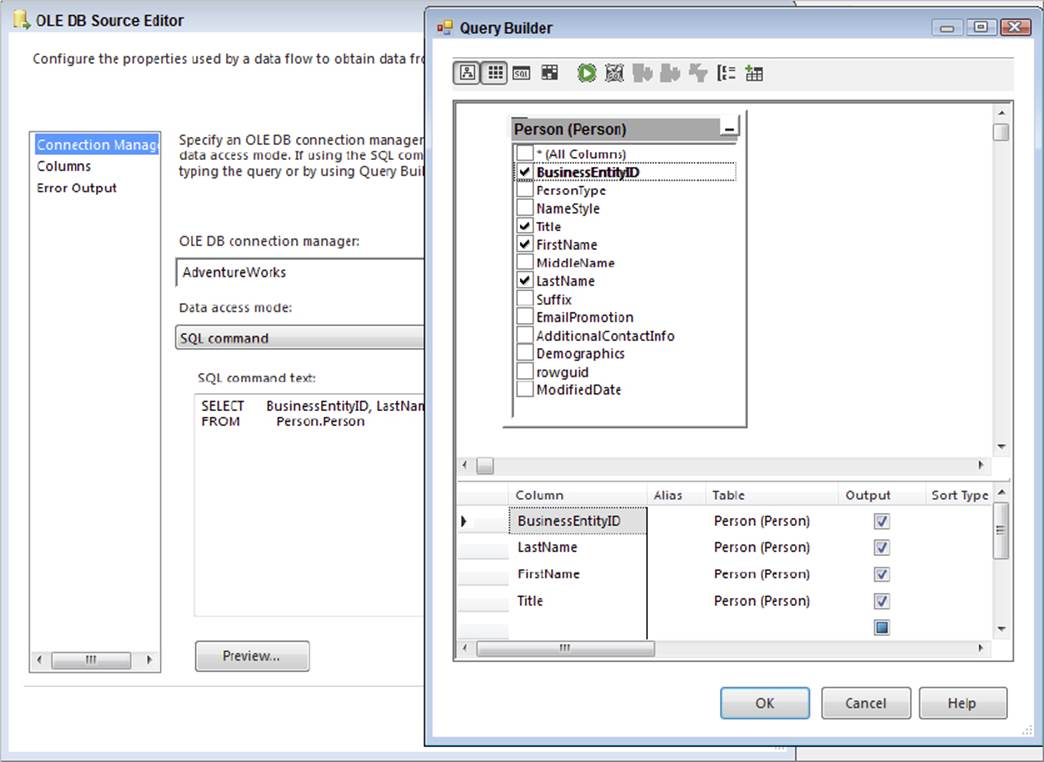
FIGURE 13-2

If you forget to use the query option or you use a SELECT * while using the query option and do not need the extraneous columns, SSIS will gently remind you during the execution of the package. The Data Flow Task’s pipeline recognizes the unused columns and throws warning events when the package runs. These messages provide an easy way to verify your column listing and performance tune your package. When running the package in debug mode, you can see the messages on the Progress tab, as shown in Figure 13-3. An example full message states: "[SSIS.Pipeline] Warning: The output column "PersonType" (31) on output "OLE DB Source Output" (29) and component "Table Option Source - Bad Practice" (18) is not subsequently used in the Data Flow task. Removing this unused output column can increase Data Flow task performance." This reminds you to remove the column PersonType from the source query to prevent the warning from reoccurring and affecting your future package executions.

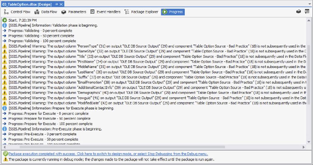
FIGURE 13-3

NOTE When using other SSIS sources, such as the Flat File Source, you do not have the option of selecting specific columns or rows with a query. Therefore, you will need to use the method of unchecking the columns to filter these sources.

WHERE Is Your Friend

As an ancillary to the previous tenet, the WHERE clause (also called the query predicate) is one of the most useful tools you can use to increase performance. Again, the table option in the Source components does not allow you to narrow down the set of columns, nor does it allow you to limit the number of rows. If all you really need are the rows from the source system that are tagged with yesterday’s date, then why stream every single other row over the wire just to throw them away once they get to SSIS? Instead, use a query with a WHERE clause to limit the number of rows being returned. As before, the less data you request, the less processing and I/O is required, and thus the faster your solution will be.

--BAD programming practice (returns 11 columns, 121,317 rows)

SELECT * FROM Sales.SalesOrderDetail;

--BETTER programming practice (returns 6 columns, 121,317 rows)

SELECT SalesOrderID, SalesOrderDetailID, OrderQty,

ProductID, UnitPrice, UnitPriceDiscount

FROM Sales.SalesOrderDetail;

--BEST programming practice (returns 6 columns, 79 rows)

SELECT SalesOrderID, SalesOrderDetailID, OrderQty,

ProductID, UnitPrice, UnitPriceDiscount

FROM Sales.SalesOrderDetail

WHERE ModifiedDate = '2008-07-01';

NOTE All code samples in this chapter are available as part of the Chapter 13 code download for the book at http://www.wrox.com/go/prossis2014.

In case it is not clear, Figure 13-4 shows how you would use this SELECT statement (and the other queries discussed next) in the context of SSIS. Drop an OLE DB or ADO.NET Source Component onto the Data Flow design surface, point it at the source database (which is AdventureWorks in this case), select the SQL command option, and plug in the preceding query.

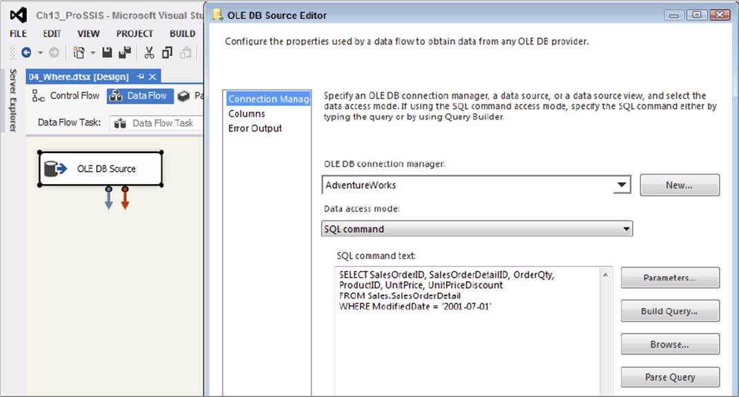
FIGURE 13-4

Transform during Extract

The basic message here is to do some of your transformations while you are extracting. This is not a viable approach for every single transformation you intend to do — especially if your ETL solution is used for compliance reasons, and you want to specifically log any errors in the data — but it does make sense for primitive operations, such as trimming whitespace, converting magic numbers to NULLs, sharpening data types, and even something as simple as providing a friendlier column name.

NOTE A magic number is a value used to represent the “unknown” or NULL value in some systems. This is generally considered bad database design practice; however, it is necessary in some systems that don’t have the concept of a NULL state. For instance, you may be using a source database for which the data steward could not assign the value “Unknown” or NULL to, for example, a date column, so instead the operators plugged in 1999/12/31, not expecting that one day the “magic number” would suddenly gain meaning!

The practice of converting data values to the smallest type that can adequately represent them is called data sharpening. In one of the following examples, you convert a DECIMAL(37,0) value to BIT because the column only ever contains the values 0 or1, as it is more efficient to store and process the data in its smallest (sharpest) representation.

Many data issues can be cleaned up as you’re extracting the data, before it even gets to SSIS. This does not mean you physically fix the data in the source system (though that would be an ideal solution).

NOTE The best way to stop bad data from reaching your source system is to restrict the entry of the data in operational applications by adding validation checks, but that is a topic beyond the scope of this book.

To fix the extraction data means you will need to write a query smart enough to fix some basic problems and send the clean data to the end user or the intended location, such as a data warehouse. If you know you are immediately going to fix dirty data in SSIS, fix it with the SQL query so SSIS receives it clean from the source.

By following this advice you can offload the simple cleanup work to the SQL Server database engine, and because it is very efficient at doing this type of set-based work, this can improve your ETL performance, as well as lower the package’s complexity. A drawback of this approach is that data quality issues in your source systems are further hidden from the business, and hidden problems tend to not be fixed!

To demonstrate this concept, imagine you are pulling data from the following source schema. The problems demonstrated in this example are not merely illustrative; they reflect some real-world issues that the authors have seen.

If you retrieve the native data into SSIS from the source just described, it will obediently generate the corresponding pipeline structures to represent this data, including the multi-byte decimal ACTIVE_IND column that will only ever contain the values 1 or 0. Depending on the number of rows in the source, allowing this default behavior incurs a large amount of processing and storage overhead. All the data issues described previously will be brought through to SSIS, and you will have to fix them there. Of course, that may be your intention, but you could make your life easier by dealing with them as early as possible.

Here is the default query that you might design:

--Old Query

SELECT [BusinessEntityID]

,[FirstName]

,[EmailPromotion]

FROM [AdventureWorks].[Person].[Person]

You can improve the robustness, performance, and intention of the preceding query. In the spirit of the “right tool for the right job,” you clean the data right inside the query so that SSIS receives it in a cleaner state. Again, you can use this query in a Source component, rather than use the table method or plug in a default SELECT * query:

--New Query

SELECT

--Cast the ID to an Int and use a friendly name

cast([BusinessEntityID] as int) as BusinessID

--Trim whitespaces, convert empty strings to Null

,NULLIF(LTRIM(RTRIM(FirstName)), '') AS FirstName

--Cast the Email Promotion to a bit

,cast((Case EmailPromotion When 0 Then 0 Else 1 End) as bit) as EmailPromoFlag

FROM [AdventureWorks].[Person].[Person]

--Only load the dates you need

Where [ModifiedDate] > '2008-12-31'

Let’s look at what you have done here:

· First, you have cast the BusinessEntityID column to a 4-byte integer. You didn’t do this conversion in the source database itself; you just converted its external projection. You also gave the column a friendlier name that your ETL developers many find easier to read and remember.

· Next, you trimmed all the leading and trailing whitespace from the FirstName column. If the column value were originally an empty string (or if after trimming it ended up being an empty string), then you convert it to NULL.

· You sharpened the EmailPromotion column to a Boolean (BIT) column and gave it a name that is simpler to understand.

· Finally, you added a WHERE clause in order to limit the number of rows.

What benefit did you gain? Well, because you did this conversion in the source extraction query, SSIS receives the data in a cleaner state than it was originally. Of course, there are bound to be other data quality issues that SSIS will need to deal with, but at least you can get the trivial ones out of the way while also improving basic performance. As far as SSIS is concerned, when it sets up the pipeline column structure, it will use the names and types represented by the query. For instance, it will believe the IsActive column is (and always has been) a BIT — it doesn’t waste any time or space treating it as a 17-byte DECIMAL. When you execute the package, the data is transformed inside the SQL engine, and SSIS consumes it in the normal manner (albeit more efficiently because it is cleaner and sharper).

You also gave the columns friendlier names that your ETL developers may find more intuitive. This doesn’t add to the performance, but it costs little and makes your packages easier to understand and maintain. If you are planning to use the data in a data warehouse and eventually in an Analysis Services cube, these friendly names will make your life much easier in your cube development.

The results of these queries running in a Data Flow in SSIS are very telling. The old query returns over 19,000 rows, and it took about 0.3 seconds on the test machine. The new query returned only a few dozen rows and took less than half the time of the old query. Imagine this was millions of rows or even billions of rows; the time savings would be quite significant. So query tuning should always be performed when developing SSIS Data Flows.

Many ANDs Make Light Work

OK, that is a bad pun, but it’s also relevant. What this tenet means is that you should let the SQL engine combine different data sets for you where it makes sense. In technical terms, this means do any relevant JOINs, UNIONs, subqueries, and so on directly in the extraction query.

That does not mean you should use relational semantics to join rows from the source system to the destination system or across heterogeneous systems (even though that might be possible) because that will lead to tightly coupled and fragile ETL design. Instead, this means that if you have two or more tables in the same source database that you are intending to join using SSIS, then JOIN or UNION those tables together as part of the SELECT statement.

For example, you may want to extract data from two tables — SalesQ1 and SalesQ2 — in the same database. You could use two separate SSIS Source components, extract each table separately, then combine the two data streams in SSIS using a Union All Component, but a simpler way would be to use a single Source component that uses a relational UNION ALL operator to combine the two tables directly:

--Extraction query using UNION ALL

SELECT --Get data from Sales Q1

SalesOrderID,

SubTotal

FROM Sales.SalesQ1

UNION ALL --Combine Sales Q1 and Sales Q2

SELECT --Get data from Sales Q2

SalesOrderID,

SubTotal

FROM Sales.SalesQ2

Here is another example. In this case, you need information from both the Product and the Subcategory table. Instead of retrieving both tables separately into SSIS and joining them there, you issue a single query to SQL and ask it to JOIN the two tables for you (see Chapter 7 for more information):

--Extraction query using a JOIN

SELECT

p.ProductID,

p.[Name] AS ProductName,

p.Color AS ProductColor,

sc.ProductSubcategoryID,

sc.[Name] AS SubcategoryName

FROM Production.Product AS p

INNER JOIN --Join two tables together

Production.ProductSubcategory AS sc

ON p.ProductSubcategoryID = sc.ProductSubcategoryID;

SORT in the Database

SQL Server has intimate knowledge of the data stored in its tables, and as such it is highly efficient at operations such as sorting — especially when it has indexes to help it do the job. While SSIS allows you to sort data in the pipeline, you will find that for large data sets SQL Server is more proficient. As an example, you may need to retrieve data from a table, then immediately sort it so that a Merge Join Transformation can use it (the Merge Join Transformation requires pre-sorted inputs). You could sort the data in SSIS by using the Sort Transformation, but if your data source is a relational database, you should try to sort the data directly during extraction in the SELECT clause. Here is an example:

--Extraction query using a JOIN and an ORDER BY

SELECT

p.ProductID,

p.[Name] AS ProductName,

p.Color AS ProductColor,

sc.ProductSubcategoryID,

sc.[Name] AS SubcategoryName

FROM

Production.Product AS p

INNER JOIN --Join two tables together

Production.ProductSubcategory AS sc

ON p.ProductSubcategoryID = sc.ProductSubcategoryID

ORDER BY --Sorting clause

p.ProductID,

sc.ProductSubcategoryID;

In this case, you are asking SQL Server to pre-sort the data so that it arrives in SSIS already sorted. Because SQL Server is more efficient at sorting large data sets than SSIS, this may give you a good performance boost. The Sort Transformation in SSIS must load all of the data in memory; therefore, it is a fully blocking asynchronous transform that should be avoided whenever possible. See Chapter 7 for more information on this.

Note that the OLE DB and ADO.NET Source Components submit queries to SQL Server in a pass-through manner — meaning they do not parse the query in any useful way themselves. The ramification is that the Source components will not know that the data is coming back sorted. To work around this problem, you need to tell the Source components that the data is ordered, by following these steps:

1. Right-click the Source component and choose Show Advanced Editor.

2. Select the Input and Output Properties tab and click the root node for the default output (not the error output). In the property grid on the right is a property called IsSorted. Change this to True. Setting the IsSorted property to true just tells the component that the data is pre-sorted, but it does not tell it in what order.

3. Next, select the columns that are being sorted on, and assign them values as follows: If the column is not sorted, the value should be zero. If the column is sorted in ascending order, the value should be positive. If the column is sorted in descending order, the value should be negative. The absolute value of the number should correspond to the column’s position in the order list. For instance, if the query was sorted with ColumnA ascending, ColumnB descending, then you would assign the value 1 to ColumnA and the value -2 to ColumnB, with all other columns set to 0.

4. In Figure 13-5, the data is sorted by the ProductID column. Expand the Output Columns node under the default output node, and then select the ProductID column. In the property grid, set the SortKeyPosition value to 1. Now the Source component is aware that the query is returning a sorted data set; furthermore, it knows exactly which columns are used for the sorting. This sorting information will be passed downstream to the next tasks. The passing down of information allows you to use components like the Merge Join Transformation, which requires sorted inputs, without using an SSIS Sort Transformation in the Data Flow.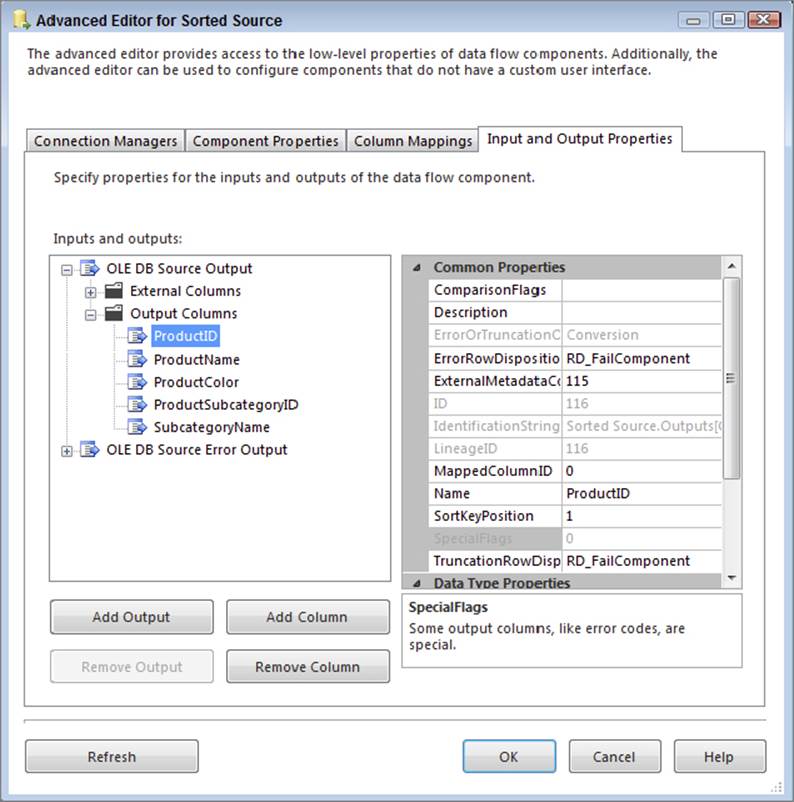

FIGURE 13-5

Be very careful when specifying the sort order — you are by contract telling the system to trust that you know what you are talking about, and that the data is in fact sorted. If the data is not sorted, or it is sorted in a manner other than you specified, then your package can act unpredictably, which could lead to data and integrity loss.

Modularize

If you find you have common queries that you keep using, then try to encapsulate those queries in the source system. This statement is based on ideal situations; in the real world you may not be allowed to touch the source system, but if you can, then there is a benefit. Encapsulating the queries in the source system entails creating views, procedures, and functions that read the data — you are not writing any data changes into the source. Once the (perhaps complex) queries are encapsulated in the source, your queries can be used in multiple packages by multiple ETL developers. Here is an example:

USE SourceSystemDatabase;

GO

CREATE PROCEDURE dbo.up_DimCustomerExtract(@date DATETIME)

-- Test harness (also the query statement you'd use in the SSIS source component):

-- Sample execution: EXEC dbo.up_DimCustomerExtract '2004-12-20';

AS BEGIN

SET NOCOUNT ON;

SELECT

--Convert to INT and alias using a friendlier name

Cast(CUSTOMER_ID as int) AS CustomerID

--Trim whitespace, convert empty strings to NULL and alias

,NULLIF(LTRIM(RTRIM(CUSTOMER_NAME)), '') AS CustomerName

--Convert to BIT and use friendly alias

,Cast(ACTIVE_IND as bit) AS IsActive

,CASE

--Convert magic dates to NULL

WHEN LOAD_DATE = '9999-12-31' THEN NULL

--Convert date to smart surrogate number of form YYYYMMDD

ELSE CONVERT(INT, (CONVERT(NVARCHAR(8), LOAD_DATE, 112)))

--Alias using friendly name

END AS LoadDateID

FROM dbo.Customers

--Filter rows using input parameter

WHERE LOAD_DATE = @date;

SET NOCOUNT OFF;

END;

GO

To use this stored procedure from SSIS, you would simply call it from within an OLE DB or ADO .NET Source Component. The example shows a static value for the date parameter, but in your solution you would use a variable or expression instead, so that you could call the procedure using different date values (see Chapter 5 for more details):

EXEC dbo.up_DimCustomerExtract '2013-12-20';

Here are some notes on the benefits you have gained here:

· In this case you have encapsulated the query in a stored procedure, though you could have encased it in a user-defined function or view just as easily. A side benefit is that this complex query definition is not hidden away in the depths of the SSIS package — you can easily access it using SQL Server.

· The benefit of a function or procedure is that you can simply pass a parameter to the module (in this case @date) in order to filter the data (study the WHERE clause in the preceding code). Note, however, that SSIS Source components have difficulty parsing parameters in functions, so you may need to use a procedure instead (which SSIS has no problems with), or you can build a dynamic query in SSIS to call the function (see Chapter 5 for more information).

· If the logic of this query changes — perhaps because you need to filter in a different way, or you need to point the query at an alternative set of tables — then you can simply change the definition in one place, and all the callers of the function will get the benefit. However, there is a risk here too: If you change the query by, for example, removing a column, then the packages consuming the function might break, because they are suddenly missing a column they previously expected. Make sure any such query updates go through a formal change management process in order to mitigate this risk.

SQL Server Does Text Files Too

It is a common pattern for source systems to export nightly batches of data into text files and for the ETL solution to pick up those batches and process them. This is typically done using a Flat File Source Component in SSIS, and in general you will find SSIS is the best tool for the job. However, in some cases you may want to treat the text file as a relational source and sort it, join it, or perform calculations on it in the manner described previously. Because the text file lives on disk, and it is a file not a database, this is not possible — or is it?

Actually, it is possible! SQL Server includes a table-valued function called OPENROWSET that is an ad hoc method of connecting and accessing remote data using OLE DB from within the SQL engine. In this context, you can use it to access text data, using theOPENROWSET(BULK ...) variation of the function.

NOTE Using the OPENROWSET and OPENQUERY statements has security ramifications, so they should be used with care in a controlled environment. If you want to test this functionality, you may need to enable the functions in the SQL Server Surface Area Configuration Tool. Alternatively, use the T-SQL configuration function as shown in the following code. Remember to turn this functionality off again after testing it (unless you have adequately mitigated any security risks). See Books Online for more information.

sp_configure 'show advanced options', 1; --Show advanced configuration options

GO

RECONFIGURE;

GO

sp_configure 'Ad Hoc Distributed Queries', 1; --Switch on OPENROWSET functionality

GO

RECONFIGURE;

GO

sp_configure 'show advanced options', 0; --Remember to hide advanced options

GO

RECONFIGURE;

GO

The SQL Server documentation has loads of information about how to use these two functions, but the following basic example demonstrates the concepts. First create a text file with the following data in it. Use a comma to separate each column value. Save the text file using the name BulkImport.txt in a folder of your choice.

1,AdventureWorks

2,Acme Apples Inc

3,Contoso Traders

Next create a format file that will help SQL Server understand how your custom flat file is laid out. You can create the format file manually or you can have SQL Server generate it for you: Create a table in the database where you want to use the format file (you can delete the table later; it is just a shortcut to build the format file). Execute the following statement in SQL Server Management Studio — for this example, you are using the AdventureWorks database to create the table, but you can use any database because you will delete the table afterward. The table schema should match the layout of the file.

--Create temporary table to define the flat file schema

USE AdventureWorks

GO

CREATE TABLE BulkImport(ID INT, CustomerName NVARCHAR(50));

Now open a command prompt, navigate to the folder where you saved the BulkImport.txt file, and type the following command, replacing “AdventureWorks” with the database where you created the BulkImport table:

bcp AdventureWorks..BulkImport format nul -c -t , -x -f BulkImport.fmt -T

If you look in the folder where you created the data file, you should now have another file called BulkImport.fmt. This is an XML file that describes the column schema of your flat file — well, actually it describes the column schema of the table you created, but hopefully you created the table schema to match the file. Here is what the format file should look like:

<?xml version="1.0"?>

<BCPFORMAT xmlns="http://schemas.microsoft.com/sqlserver/2004/bulkload/format"

xmlns:xsi=http://www.w3.org/2001/XMLSchema-instance>

<RECORD>

<FIELD ID="1" xsi:type="CharTerm" TERMINATOR="," MAX_LENGTH="12"/>

<FIELD ID="2" xsi:type="CharTerm" TERMINATOR="\r\n" MAX_LENGTH="100"

COLLATION="SQL_Latin1_General_CP1_CI_AS"/>

</RECORD>

<ROW>

<COLUMN SOURCE="1" NAME="ID" xsi:type="SQLINT"/>

<COLUMN SOURCE="2" NAME="CustomerName" xsi:type="SQLNVARCHAR"/>

</ROW>

</BCPFORMAT>

Remember to delete the table (BulkImport) you created, because you don’t need it anymore. If you have done everything right, you should now be able to use the text file in the context of a relational query. Type the following query into SQL Server Management Studio, replacing the file paths with the exact folder path and names of the two files you created:

--Select data from a text file as if it was a table

SELECT

T.* --SELECT * used for illustration purposes only

FROM OPENROWSET(--This is the magic function

BULK 'c:\ProSSIS\Data\Ch13\BulkImport.txt', --Path to data file

FORMATFILE = 'c:\ProSSIS\Data\Ch13\BulkImport.fmt' --Path to format file

) AS T; --Command requires a table alias

After executing this command, you should get back rows in the same format they would be if they had come from a relational table. To prove that SQL Server is treating this result set in the same manner it would treat any relational data, try using the results in the context of more complex operations such as sorting:

--Selecting from a text file and sorting the results

SELECT

T.OrgID, --Not using SELECT * anymore

T.OrgName

FROM OPENROWSET(

BULK 'c:\ProSSIS\Data\Ch13\BulkImport.txt',

FORMATFILE = 'c:\ProSSIS\Data\Ch13\BulkImport.fmt'

) AS T(OrgID, OrgName) --For fun, give the columns different aliases

ORDER BY T.OrgName DESC; --Sort the results in descending order

You can declare if and how the text file is pre-sorted. If the system that produced the text file did so in a sorted manner, then you can inform SQL Server of that fact. Note that this is a contract from you, the developer, to SQL Server. SQL Server uses something called a streaming assertion when reading the text file to double-check your claims, but in some cases this can greatly improve performance. Later you will see how this ordering contract helps with the MERGE operator, but here’s a simple example to demonstrate the savings.

Run the following query. Note how you are asking for the data to be sorted by OrgID this time. Also note that you have asked SQL Server to show you the query plan that it uses to run the query:

SET STATISTICS PROFILE ON; --Show query plan

SELECT

T.OrgID,

T.OrgName

FROM OPENROWSET(

BULK 'c:\ProSSIS\Data\Ch13\BulkImport.txt',

FORMATFILE = 'c:\ProSSIS\Data\Ch13\BulkImport.fmt'

) AS T(OrgID, OrgName)

ORDER BY T.OrgID ASC; --Sort the results by OrgID

SET STATISTICS PROFILE OFF; --Hide query plan

Have a look at the following query plan that SQL Server generates. The query plan shows the internal operations SQL Server has to perform to generate the results. In particular, note the second operation, which is a SORT:

SELECT <...snipped...>

|--Sort(ORDER BY:([BULK].[OrgID] ASC))

|--Remote Scan(OBJECT:(STREAM))

This is obvious and expected; you asked SQL Server to sort the data, and it does so as requested. Here’s the trick: In this case, the text file happened to be pre-sorted by OrgID anyway, so the sort you requested was actually redundant. (Note the text data file; the ID values increase monotonically from 1 to 3.)

To prove this, type the same query into SQL again, but this time use the OPENROWSET(... ORDER) clause:

SET STATISTICS PROFILE ON; --Show query plan

SELECT

T.OrgID,

T.OrgName

FROM OPENROWSET(

BULK 'c:\ProSSIS\Data\Ch13\BulkImport.txt',

FORMATFILE = 'c:\ProSSIS\Data\Ch13\BulkImport.fmt',

ORDER (OrgID ASC) --Declare the text file is already sorted by OrgID

)AS T(OrgID, OrgName)

ORDER BY T.OrgID ASC; --Sort the results by OrgID

SET STATISTICS PROFILE OFF; --Hide query plan

Once again you have asked for the data to be sorted, but you have also contractually declared that the source file is already pre-sorted. Have a look at the new query plan. Here’s the interesting result: Even though you asked SQL Server to sort the result in the finalORDER BY clause, it didn’t bother doing so because you indicated (and it confirmed) that the file was already ordered as such:

SELECT <...snipped...>

|--Assert <...snipped...>

|--Sequence Project(<...snipped...>)

|--Segment

|--Remote Scan(OBJECT:(STREAM))

As you can see, there is no SORT operation in the plan. There are other operators, but they are just inexpensive assertions that confirm the contract you specified is true. For instance, if a row arrived that was not ordered in the fashion you declared, the statement would fail. The streaming assertion check is cheaper than a redundant sort operation, and it is good logic to have in place in case you got the ordering wrong, or the source system one day starts outputting data in a different order than you expected.

So after all that, why is this useful to SSIS? Here are a few examples:

· You may intend to load a text file in SSIS and then immediately join it to a relational table. Now you could do all that within one SELECT statement, using a single OLE DB or ADO .NET Source Component.

· Some of the SSIS components expect sorted inputs (the Merge Join Component, for example). Assuming the source is a text file, rather than sort the data in SSIS you can sort it in SQL Server. If the text file happens to be pre-sorted, you can declare it as such and save even more time and expense.

· The Lookup Transformation can populate data from almost anywhere (see Chapter 7). This may still prove a useful technique in some scenarios.

WARNING Using OPENROWSET to select from a text file should be used only as a temporary solution, as it has many downfalls. First, there are no indexes on the file, so performance is going to be degraded severely. Second, if the sourcetype=“warning” data file changes in structure (for instance, a column is dropped), and you don’t keep the format file in sync, then the query will fail. Third, if the format file is deleted or corrupted, the query will also fail. This technique can be used when SSIS is not available or does not meet your needs. In most cases, loading the file into a table with SSIS and then querying that table will be your best option.

Using Set-Based Logic

Cursors are infamous for being very slow. They usually perform row-by-row operations that are time-consuming. The SQL Server relational database engine, along with SSIS, performs much faster in set-based logic. The premise here is simple: Avoid any use of cursors like the plague. Cursors are nearly always avoidable, and they should be used only as a final resort. Try out the following features and see if they can help you build efficient T-SQL operations:

· Common table expressions (CTEs) enable you to modularize subsections of your queries, and they also support recursive constructs, so you can, for instance, retrieve a self-linked (parent-child) organizational hierarchy using a single SQL statement.

· Table-valued parameters enable you to pass arrays into stored procedures as variables. This means that you can program your stored procedure logic using the equivalent of dynamic arrays.

· UNION is now joined by its close cousins, INTERSECT and EXCEPT, which completes the primitive set of operations you need to perform set arithmetic. UNION joins two rowsets together, INTERSECT finds their common members, and EXCEPT finds the members that are present in one rowset but not the other.

The following example brings all these ideas together. In this example scenario, suppose you have two tables of data, both representing customers. The challenge is to group the data into three subsets: one set containing the customers who exist in the first table only, the second set containing customers who exist in the second table only, and the third set containing the customers who exist in both tables. The specific example illustrates the power and elegance of common table expressions (CTEs) and set-arithmetic statements. If you remember Venn diagrams from school, what you are trying to achieve is the relational equivalent of the diagram shown in Figure 13-6.

FIGURE 13-6

Following is a single statement that will partition the data as required. This statement is not meant to convey good programming practice, because it is not the most optimal or concise query you could write to derive these results. It is simply meant to demonstrate the manner in which these constructs can be used. By studying the verbose form, you can appreciate the elegance, composability, and self-documenting nature of the syntax.

For convenience you will use related tables from AdventureWorks and AdventureWorksDW. Note the use of multiple CTE structures to generate intermediate results (though the query optimizer is smart enough to not execute the statements separately). Also notice the use of UNION, EXCEPT, and INTERSECT to derive specific results:

WITH SourceRows AS ( --CTE containing all source rows

SELECT TOP 1000 AccountNumber

FROM AdventureWorks.Sales.Customer

ORDER BY AccountNumber

),

DestinationRows(AccountNumber) AS ( --CTE containing all destination rows

SELECT CustomerAlternateKey

FROM AdventureWorksDW.dbo.DimCustomer

),

RowsInSourceOnly AS ( --CTE: rows where AccountNumber is in source only

SELECT AccountNumber FROM SourceRows --select from previous CTE

EXCEPT --EXCEPT means 'subtract'

SELECT AccountNumber FROM DestinationRows --select from previous CTE

),

RowsInSourceAndDestination AS( --CTE: AccountNumber in both source & destination

SELECT AccountNumber FROM SourceRows

INTERSECT --INTERSECT means 'find the overlap'

SELECT AccountNumber FROM DestinationRows

),

RowsInDestinationOnly AS ( --CTE: AccountNumber in destination only

SELECT AccountNumber FROM DestinationRows

EXCEPT --Simply doing the EXCEPT the other way around

SELECT AccountNumber FROM SourceRows

),

RowLocation(AccountNumber, Location) AS ( --Final CTE

SELECT AccountNumber, 'Source Only' FROM RowsInSourceOnly

UNION ALL --UNION means 'add'

SELECT AccountNumber, 'Both' FROM RowsInSourceAndDestination

UNION ALL

SELECT AccountNumber, 'Destination Only' FROM RowsInDestinationOnly

)

SELECT * FROM RowLocation --Generate final result

ORDER BY AccountNumber;

Here is a sample of the results:

AccountNumber Location

----------- -----------

AW00000700 Source Only

AW00000701 Source Only

AW00011000 Both

. . .

AW00011298 Both

AW00011299 Destination Only

AW00011300 Destination Only

SQL Server provides many powerful tools for use in your data extraction arsenal. Learn about them and then start using the SQL Server relational database engine and SSIS in concert to deliver optimal extraction routines. The list presented previously is not exhaustive; you can use many other similar techniques to improve the value of the solutions you deliver.

DATA LOADING

This section focuses on data loading. Many of the same techniques presented in the data extraction section apply here too, so the focus is on areas that have not been covered before.

Database Snapshots

Database snapshots were introduced as a way to persist the state of a database at a specific point in time. The underlying technology is referred to as copy-on-first-write, which is a fancy way of saying that once you create the database snapshot, it is relatively cheap to maintain because it only tracks things that have changed since the database snapshot was created. Once you have created a database snapshot, you can change the primary database in any way — for instance, changing rows, creating indexes, and dropping tables. If at any stage you want to revert all your changes back to when you created the database snapshot, you can do that very easily by doing a database restore using the database snapshot as the media source.

In concept, the technology sounds very similar to backup and restore, the key difference being that this is a completely online operation, and depending on your data loads, the operations can be near instantaneous. This is because when you create the snapshot, it is a metadata operation only — you do not physically “back up” any data. When you “restore” the database from the snapshot, you do not restore all the data; rather, you restore only what has changed in the interim period.

This technique proves very useful in ETL when you want to prototype any data changes. You can create a package that makes any data changes you like, confident in the knowledge that you can easily roll back the database to a clean state in a short amount of time. Of course, you could achieve the same goals using backup and restore (or transactional semantics), but those methods typically have more overhead and/or take more time. Snapshots may also be a useful tool in operational ETL; you can imagine a scenario whereby a snapshot is taken before an ETL load and then if there are any problems, the data changes can be easily rolled back.

There is a performance overhead to using snapshots, because you can think of them as a “live” backup. Any activity on the source database incurs activity on the snapshot database, because the first change to any database page causes that page to be copied to the database snapshot. Any subsequent changes to the same page do not cause further copy operations but still have some overhead due to the writing to both source and snapshot. You need to test the performance overhead in the solutions you create, though you should expect to see an overhead of anywhere from 5 percent to 20 percent.

Because you are writing data to the destination database in this section, it is useful to create a database snapshot so you can roll back your changes very easily. Run this complete script:

--Use a snapshot to make it simple to rollback the DML

USE master;

GO

--To create a snapshot you need to close all other connections on the DB

ALTER DATABASE [AdventureWorksDW] SET SINGLE_USER WITH ROLLBACK IMMEDIATE;

ALTER DATABASE [AdventureWorksDW] SET MULTI_USER;

--Check if there is already a snapshot on this DB

IF EXISTS (SELECT [name] FROM sys.databases

WHERE [name] = N'AdventureWorksDW_Snapshot') BEGIN

--If so RESTORE the database from the snapshot

RESTORE DATABASE AdventureWorksDW

FROM DATABASE_SNAPSHOT = N'AdventureWorksDW_Snapshot';

--If there were no errors, drop the snapshot

IF @@error = 0 DROP DATABASE [AdventureWorksDW_Snapshot];

END; --if

--OK, let's create a new snapshot on the DB

CREATE DATABASE [AdventureWorksDW_Snapshot] ON (

NAME = N'AdventureWorksDW_Data',

--Make sure you specify a valid location for the snapshot file here

FILENAME = N'c:\ProSSIS\Data\Ch13\AdventureWorksDW_Data.ss')

AS SNAPSHOT OF [AdventureWorksDW];

GO

The script should take only a couple of seconds to run. It creates a database file in the specified folder that it tagged as being a snapshot of the AdventureWorksDW database. You can run the following command to list all the database snapshots on the server:

--List database snapshots

SELECT

d.[name] AS DatabaseName,

s.[name] AS SnapshotName

FROM sys.databases AS s

INNER JOIN sys.databases AS d

ON (s.source_database_id = d.database_id);

You should now have a snapshot called “AdventureWorksDW_Snapshot.” This snapshot is your “live backup” of AdventureWorksDW. Once you have ensured that the database snapshot is in place, test its functionality by changing some data or metadata in AdventureWorksDW. For instance, you can create a new table in the database and insert a few rows:

--Create a new table and add some rows

USE AdventureWorksDW;

GO

CREATE TABLE dbo.TableToTestSnapshot(ID INT);

GO

INSERT INTO dbo.TableToTestSnapshot(ID) SELECT 1 UNION SELECT 2 UNION SELECT 3;

You can confirm the table is present in the database by running this statement. You should get back three rows:

--Confirm the table exists and has rows

SELECT * FROM dbo.TableToTestSnapshot;

Now you can test the snapshot rollback functionality. Imagine that the change you made to the database had much more impact than just creating a new table (perhaps you dropped the complete sales transaction table, for instance) and you now want to roll the changes back. Execute the same script that you used to originally create the snapshot; you will notice that the script includes a check to ensure that the snapshot exists; then, if so, it issues a RESTORE ... FROM DATABASE_SNAPSHOT command.

After running the script, try running the SELECT command again that returned the three rows. You should get an error saying the table “TableToTestSnapshot” does not exist. This is good news; the database has been restored to its previous state! Of course, this same logic applies whether you created a table or dropped one, added or deleted rows, or performed just about any other operation. The really cool benefit is that it should have taken only a couple of seconds to run this “live restore.”

As part of the original snapshot script, the database was rolled back, but the script should also have created a new snapshot in the old one’s place. Make sure the snapshot is present before continuing with the next sections, because you want to make it simple to roll back any changes you make.

Not only can you use database snapshots for prototyping, you can add tasks to your regularly occurring ETL jobs to create the snapshots — and even restore them if needed! A solution that uses this methodology is robust enough to correct its own mistakes and can be part of an enterprise data warehouse solution.

The MERGE Operator

If your source data table is conveniently partitioned into data you want to insert, data you want to delete, and data you want to update, then it is simple to use the INSERT, UPDATE, and DELETE statements to perform the respective operations. However, it is often the case that the data is not presented to you in this format. More often than not you have a source system with a range of data that needs to be loaded, but you have no way of distinguishing which rows should be applied in which way. The source contains a mix of new, updated, and unchanged rows.

One way you can solve this problem is to build logic that compares each incoming row with the destination table, using a Lookup Transformation (see Chapter 7 for more information). Another way to do this would be to use Change Data Capture (see Chapter 11 for more information) to tell you explicitly which rows and columns were changed, and in what way.

There are many other ways of doing this too, but if none of these methods are suitable, you have an alternative, which comes in the form of the T-SQL operator called MERGE (also known in some circles as “upsert” because of its mixed Update/Insert behavior).

The MERGE statement is similar in usage to the INSERT, UPDATE, and DELETE statements; however, it is more useful in that it can perform all three of their duties within the same operation. Here is pseudocode to represent how it works; after this you will delve into the real syntax and try some examples:

MERGE INTO Destination

Using these semantics:

{

<all actions optional>

If a row in the Destination matches a row in the Source then: UPDATE

If a row exists in the Source but not in the Destination then: INSERT

If a row exists in the Destination but not in the Source then: DELETE

}

FROM Source;

As you can see, you can issue a single statement to SQL Server, and it is able to figure out on a row-by-row basis which rows should be INSERT-ed, UPDATE-ed, and DELETE-ed in the destination. This can provide a huge time savings compared to doing it the old way: issuing two or three separate statements to achieve the same goal. Note that SQL Server is not just cleverly rewriting the MERGE query back into INSERT and UPDATE statements behind the scenes; this functionality is a DML primitive deep within the SQL core engine, and as such it is highly efficient.

Now you are going to apply this knowledge to a real set of tables. In the extraction section of this chapter you used customer data from AdventureWorks and compared it to data in AdventureWorksDW. There were some rows that occurred in both tables, some rows that were only in the source, and some rows that were only in the destination. You will now use MERGE to synchronize the rows from AdventureWorks to AdventureWorksDW so that both tables contain the same data.

This is not a real-world scenario because you would not typically write rows directly from the source to the destination without cleaning and shaping the data in an ETL tool like SSIS, but for the sake of convenience the example demonstrates the concepts.

First, you need to add a new column to the destination table so you can see what happens after you run the statement. This is not something you would need to do in the real solution.

USE AdventureWorksDW;

GO

--Add a column to the destination table to help us track what happened

--You would not do this in a real solution, this just helps the example

ALTER TABLE dbo.DimCustomer ADD Operation NVARCHAR(10);

GO

Now you can run the MERGE statement. The code is commented to explain what it does. The destination data is updated from the source in the manner specified by the various options. There are blank lines between each main section of the command to improve readability, but keep in mind that this is a single statement:

USE AdventureWorksDW;

GO

--Merge rows from source into the destination

MERGE

--Define the destination table

INTO AdventureWorksDW.dbo.DimCustomer AS [Dest] --Friendly alias

--Define the source query

USING (

SELECT AccountNumber AS CustomerAlternateKey,

--Keep example simple by using just a few data columns

p.FirstName,

p.LastName

FROM AdventureWorks.Sales.Customer c

INNER JOIN AdventureWorks.Person.Person p on c.PersonID=p.BusinessEntityID

) AS [Source] --Friendly alias

--Define the join criteria (how SQL matches source/destination rows)

ON [Dest].CustomerAlternateKey = [Source].CustomerAlternateKey

--If the same key is found in both the source & destination

WHEN MATCHED

--For *illustration* purposes, only update every second row

--AND CustomerAlternateKey % 2 = 0

--Then update data values in the destination

THEN UPDATE SET

[Dest].FirstName = [Source].FirstName ,

[Dest].LastName = [Source].LastName,

[Dest].Operation = N'Updated'

--Note: <WHERE CustomerAlternateKey =...> clause is implicit

--If a key is in the source but not in the destination

WHEN NOT MATCHED BY TARGET

--Then insert row into the destination

THEN INSERT

(

GeographyKey, CustomerAlternateKey, FirstName,

LastName, DateFirstPurchase, Operation

)

VALUES

(

1, [Source].CustomerAlternateKey, [Source].FirstName,

[Source].LastName, GETDATE(), N'Inserted'

)

--If a key is in the destination but not in the source...

WHEN NOT MATCHED BY SOURCE

--Then do something relevant, say, flagging a status field

THEN UPDATE SET

[Dest].Operation = N'Deleted';

--Note: <WHERE ContactID =...> clause is implicit

--Alternatively you could have deleted the destination row

--but in AdventureWorksDW that would fail due to FK constraints

--WHEN NOT MATCHED BY SOURCE THEN DELETE;

GO

After running the statement, you should get a message in the query output pane telling you how many rows were affected:

(19119 row(s) affected)

You can now check the results of the operation by looking at the data in the destination table. If you scroll through the results you should see each row’s Operation column populated with the operation that was applied to it:

--Have a look at the results

SELECT CustomerAlternateKey, DateFirstPurchase, Operation

FROM AdventureWorksDW.dbo.DimCustomer;

Here is a subset of the results. For clarity, the different groups of rows have been separated in this book by blank lines:

CustomerAlternateKey DateFirstPurchase Operation

-------------------- ----------------------- -----------

AW00019975 2002-04-11 00:00:00.000 NULL

AW00019976 2003-11-27 00:00:00.000 Updated

AW00019977 2002-04-26 00:00:00.000 NULL

AW00019978 2002-04-20 00:00:00.000 Deleted

AW00019979 2002-04-22 00:00:00.000 Deleted

AW00008000 2008-02-24 20:48:12.010 Inserted

AW00005229 2008-02-24 20:48:12.010 Inserted

AW00001809 2008-02-24 20:48:12.010 Inserted

As you can see, a single MERGE statement has inserted, updated, and deleted rows in the destination in the context of just one operation. The reason why some of the updates could show a NULL operation is if a predicate was used in the WHEN MATCHED section to only UPDATEevery second row.

Note that the source query can retrieve data from a different database (as per the example); furthermore, it can even retrieve data using the OPENROWSET() function you read about earlier. However, MERGE requires sorting the source data stream on the join key; SQL Server will automatically sort the source data for you if required, so ensure that the appropriate indexes are in place for a more optimal experience. These indexes should be on the join key columns. Do not confuse this operator with the Merge Join Transformation in SSIS.

If the source query happens to be of the form OPENROWSET(BULK...) — in other words, you are reading from a text file — then make sure you have specified any intrinsic sort order that the text file may already have. If the text file is already sorted in the same manner as the order required for MERGE (or you can ask the source extract system to do so), then SQL is smart enough to not incur a redundant sort operation.

The MERGE operator is a very powerful technique for improving mixed-operation data loads, but how do you use it in the context of SSIS?

If you do not have the benefit of Change Data Capture (discussed in Chapter 11) and the data sizes are too large to use the Lookup Transformation in an efficient manner (see Chapter 7), then you may have to extract your data from the source, clean and shape it in SSIS, and then dump the results to a staging table in SQL Server. From the staging table, you now need to apply the rows against the true destination table. You could certainly do this using two or three separate INSERT, UPDATE, and DELETE statements — with each statement JOIN-ing the staging table and the destination table together in order to compare the respective row and column values. However, you can now use a MERGE statement instead. The MERGE operation is more efficient than running the separate statements, and it is more intentional and elegant to develop and maintain. This is also more efficient with larger data sets than the SCD wizard and its OLE DB Command Transformation approach.

Make sure you execute the original snapshot script again in order to undo the changes you made in the destination database.

SUMMARY

As this chapter has shown, you can take advantage of many opportunities to use SQL in concert with SSIS in your ETL solution. The ideas presented in this chapter are not exhaustive; many other ways exist to increase your return on investment using the Microsoft data platform. Every time you find a way to use a tool optimized for the task at hand, you can lower your costs and improve your efficiencies. There are tasks that SSIS is much better at doing than the SQL Server relational database engine, but the opposite statement applies too. Make sure you think about which tool will provide the best solution when building ETL solutions; the best solutions often utilize a combination of the complete SQL Server business intelligence stack.