Professional Microsoft SQL Server 2014 Integration Services (Wrox Programmer to Programmer), 1st Edition (2014)

Chapter 14. Accessing Heterogeneous Data

WHAT’S IN THIS CHAPTER?

· Dealing with Excel and Access data

· Integrating with Oracle

· Working with XML files and web services

· Extracting from flat files

· Integrating with ODBC

WROX.COM CODE DOWNLOADS FOR THIS CHAPTER

You can find the wrox.com code downloads for this chapter at http://www.wrox.com/go/prossis2014 on the Download Code tab.

In this chapter, you will learn about importing and working with data from heterogeneous, or various non–SQL Server, sources. In today’s enterprise environments, data may exist in many diverse systems, such as Oracle, DB2, Teradata, SQL Azure, SQL Parallel Data Warehouse (PDW), Office documents, XML, or flat files, to name just a few. The data may be generated within the company, or it may be delivered through the Internet from a trading partner. Whether you need to import data from a spreadsheet to initially populate a table in a new database application or pull data from other sources for your data warehouse, accessing heterogeneous data is probably a big part of your job.

You can load data into SQL Server using SSIS through any ODBC-compliant, OLE DB–compliant, or ADO.NET managed source. Many ODBC, OLE DB, and .NET providers are supplied by Microsoft for sources like Excel, Access, DB2, FoxPro, Sybase, Oracle, Teradata, and dBase. Others are available from database vendors. A variety of Data Source Components are found in SSIS. These include Excel, Flat File, XML, ADO.NET (which is used to connect to .NET Sources), OLE DB (which allows connections to many different types of data), and Raw File (a special source used to read data that has been previously exported to a Raw File Destination). If the supplied Data Sources do not meet your needs, you can also create custom Data Sources.

SSIS can consume many of these sources from out-of-the-box features. In addition, Microsoft has also provided a set of free downloads in the SQL Server feature pack for advanced data source extraction. They include a set of source components from Attunity, third-party components that Microsoft has licensed for use with SSIS. The Attunity connectors allow advanced sourcing from Oracle (with bulk load capabilities), Teradata, and ODBC sources.

Figure 14-1 highlights the Source Assistant within the Data Flow Toolbox. It shows the various source options within SSIS. Many of them require the installation of a client tool; the gray information window at the bottom of the figure describes where to find the additional application if required.

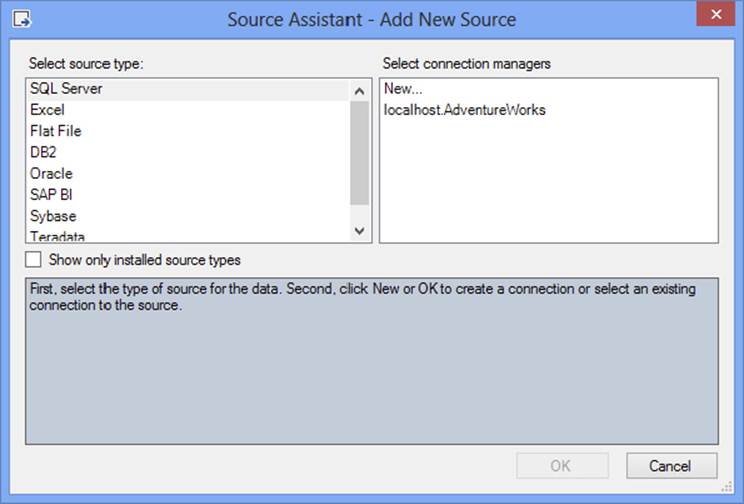
FIGURE 14-1

This chapter begins with the built-in features and walks you through accessing data from several of the most common sources. In addition to working in SSIS, you will become familiar with the differences between 32-bit and 64-bit drivers, as well as the client tools you need to install for the provider for DB2, Oracle, SAP BI, and Teradata, as available from those websites. This chapter targets the following sources:

· Excel and MS Access (versions 2013 and earlier): Excel is often used as a quick way to store data because spreadsheets are easy to set up and use. Access applications are frequently upsized to SQL Server as the size of the database and number of users increase.

· Oracle: Even companies running their business on Oracle or another of SQL Server’s competitors sometimes make use of SQL Server because of its cost-effective reporting and business intelligence solutions.

· XML and Web Services: XML and web services (which is XML delivered through HTTP) are standards that enable very diverse systems to share data. The XML Data Source enables you to work with XML as you would with almost any other source of data.

· Flat Files: Beyond just standard delimited files, SSIS can parse flat files of various types and code page encoding, which allows files to be received from and exported to different operating systems and non-Windows-based systems. This reduces the need to convert flat files before or after working with them in SSIS.

· ODBC: Many organizations maintain older systems that use legacy ODBC providers for data access. Because of the complexities and cost of migrating systems to newer versions, ODBC is still a common source.

· Teradata: Teradata is a data warehouse database engine that scales out on multiple nodes. Large organizations that can afford Teradata’s licensing and ongoing support fees often use it for centralized warehouse solutions.

· Other Heterogeneous Sources: The sources listed previously are the most common; however, this only touches on the extent of Data Sources that SSIS can access. The last section of this chapter provides third-party resources for when you are trying to access other sources such as SAP or Sybase.

EXCEL AND ACCESS

SSIS deals with Excel and Access data in a similar fashion because they use the same underlying provider technology for data access. For Microsoft Office 2003 and earlier, the data storage technology is called the JET Engine, which stands for Join Engine Technology; therefore, when you access these legacy releases of Excel or Access, you will be using the JET OLE DB Provider (32-bit only).

Office 2007 introduced a new engine called ACE that is essentially a newer version of the JET but supports the new file formats of Excel and Access. ACE stands for Access Engine and is used for Office 2007 and later. In addition, with the release of Office 2010, Microsoft provided a 64-bit version of the ACE provider. You will find both the 32-bit and 64-bit drivers under the name “Microsoft Office 12.0 Access Database Engine OLE DB Provider” in the OLE DB provider list. Therefore, when connecting to Access or Excel in these versions, you will use the ACE OLE DB Provider. If you have the 64-bit version of Office 2010 or 2013 installed, the next section will also review working with the 32-bit provider, because it can be confusing.

Later in this section you will learn how to connect to both Access and Excel for both the JET and ACE engines.

64-Bit Support

In older versions of Office (Office 2007 and earlier), only a 32-bit driver was available. That meant if you wanted to extract data from Excel or Access, you had to run SSIS in 32-bit mode. Beginning with Office 2010, however, a 64-bit version of the Office documents became available that enables you to extract data from Excel and Access using SSIS on a 64-bit server in native mode. In order to use the 64-bit versions of the ACE engine, you need to install the 64-bit access provider either by installing the 64-bit version of Microsoft Office 2010 or later or by installing the 64-bit driver from Microsoft’s download site: http://www.microsoft.com/en-us/download/details.aspx?id=39358.

However, even though a 64-bit version of the ACE provider is available, you cannot develop packages with the 64-bit driver. This is because Visual Studio is a 32-bit application and is unable to see a 64-bit driver. With ACE, if you try to install both 32-bit and 64-bit, you will receive the error shown in Figure 14-2.

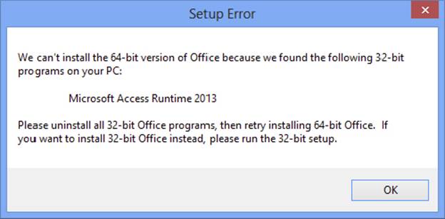
FIGURE 14-2

Therefore, the 64-bit driver can be used for a test or production server where packages are not executed through the design-time environment. The approach to using the 64-bit driver is to design your package with the 32-bit driver and then deploy your package to a server that has the 64-bit ACE driver installed.

To be sure, SSIS can run natively on a 64-bit machine (just like it can on a 32-bit machine). This means that when the operating system is running the X64 version of Windows Server 2003, Windows 7, Windows 8, Windows Server 2008, or a future version of Windows Server, you can natively install and run SQL Server in the X64 architecture (an IA64 Itanium build is also available from Microsoft support). When you execute a package in either 64-bit or 32-bit mode, the driver needs to either work in both execution environments or, like the ACE provider, have the right version for either the 32-bit or 64-bit execution mode.

When you install SSIS with the native X64 installation bits, you also get the 32-bit runtime executables that you can use to run packages that need access to 32-bit drivers not supported in the 64-bit environment. When working on a 64-bit machine, you can run packages in 32-bit emulation mode through the SSDT design environment and through the 32-bit version of DTExec. In addition, when using the SSIS Server Catalog in SQL 2014, you are also able to run packages in 32-bit or 64-bit mode.

Here are the details:

· Visual Studio 2012: By default, when you are in a native 64-bit environment and you run a package, you are running the package in 64-bit mode. However, you can change this behavior by modifying the properties of your SSIS project. Figure 14-3 shows the Run64bitRuntime property on the Debugging property page. When you set this to False, the package runs in 32-bit emulation mode even though the machine is 64-bit.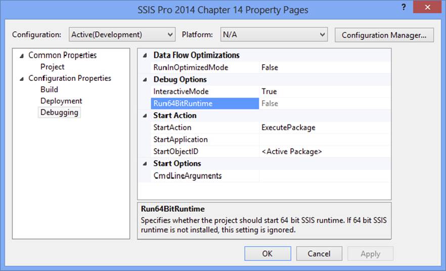

FIGURE 14-3

· 32-bit version of DTExec: By default, a 64-bit installation of SSIS references the 64-bit version of DTExec, usually found in the C:\Program Files\Microsoft SQL Server\120\DTS\Binn folder. However, a 32-bit version is also included in C:\Program Files (X86)\Microsoft SQL Server\120\DTS\Binn, and you can reference that directly if you want a package to run in 32-bit emulation mode in order to access the ACE and JET providers.

· 32-bit version for packages deployed to SSIS catalog: When running a package that has been deployed to the SSIS 2014 catalog, an advanced configuration option, “32-bit runtime,” will allow your package to be executed in legacy 32-bit execution mode. This option is available both in SQL Agent and in the package execution UI in the SSIS 2014 catalog. The default is to have this option unchecked so that packages run in 64-bit mode.

Be careful not to run all your packages in 32-bit emulation mode when running on a 64-bit machine, just the ones that need 32-bit support. The 32-bit emulation mode limits the memory accessibility and the performance. The best approach is to modularize your packages by developing more packages with less logic in them. One benefit to this is the packages that need 32-bit execution can be separated and run separately.

Working with Excel Files

Excel is a common source and destination because it is often the favorite “database” software of many people without database expertise (especially in your accounting department!). SSIS has Data Flow Source and Destination Components made just for Excel that ease the connection setup, whether connecting to Excel 2003 or earlier or to Excel 2007 or later (the JET and ACE providers).

You can be sure that these components will be used in many SSIS packages, because data is often imported from Excel files into a SQL Server database or exported into Excel for many high-level tasks such as sales forecasting. Because Excel is so easy to work with, it is common to find inconsistencies in the data. For example, while lookup lists or data type enforcement is possible to implement, it is less likely for an Excel workbook to have it in place. It’s often possible for the person entering data to type a note in a cell where a date should go. Of course, cleansing the data is part of the ETL process, but it may be even more of a challenge when importing from Excel.

Exporting to All Versions of Excel

In this section, you will use SSDT to create SSIS packages to export data to Excel files. The first example shows how to create a package that exports a worksheet that the AdventureWorks inventory staff will use to record the physical inventory counts. Follow these steps to learn how to export data to Excel:

1. Create a new SSIS package in SSDT and Rename the package Export Excel.dtsx.

2. Drag a Data Flow Task from the Toolbox to the Control Flow design area and then switch to the Data Flow tab.

3. Add an OLE DB Source Component.

4. Create a Connection Manager pointing to the AdventureWorks database.

5. Double-click the OLE DB Source Component to bring up the OLE DB Source Editor. Make sure that Connection Manager is selected on the left.

6. Choose the AdventureWorks Connection Manager for the OLE DB Connection Manager property. The data access mode should be set to SQL Command. In this case, you will write a query (Excel_Export_SQL.txt) to specify which data to export:

7. SELECT ProductID, LocationID, Shelf, Bin,

8. Null as PhysicalCount

9. FROM Production.ProductInventory

ORDER by LocationID, Shelf, Bin

10.If you select Columns in the left pane, you have the opportunity to deselect some of the columns or change the name of the output columns. Click OK to accept the configuration.

11.Drag an Excel Destination Component from the SSIS Toolbox, found under the Other Destinations grouping and drag the Data Flow Path (blue arrow on your screen) from the OLE DB Source to the Excel Destination. Double-click the Excel Destination.

12.Click the New button for the Connection Manager, and in the Excel Connection Manager window, choose Microsoft Excel 2007 from the Excel Version dropdown, and then enter the path to your destination (C:\ProSSIS\Data\Inventory_Worksheet.xlsx).

13.Select OK in the Excel Connection Manager window, and then click New on the Name of Excel sheet dropdown to create a new worksheet.

14.In the Create Table window, you can leave the name of the worksheet or change it and modify the columns as Figure 14-4 shows. Click OK to create the new worksheet.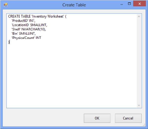

FIGURE 14-4

15.The data access mode should be set to Table or View (more about this later). Click OK to create a new worksheet with the appropriate column headings in the Excel file. Make sure that Name of the Excel sheet is set to Inventory Worksheet.

16.You must click Mappings on the left to set the mappings between the source and the destination. Each one of the Available Input Columns should match up exactly with an Available Output Column. Click OK to accept the Inventory Worksheet settings.

Run the package to export the product list. The fields selected in the Production.Inventory table will export to the Excel file, and your inventory crew members can each use a copy of this file to record their counts.

Importing from Excel 2003 and Earlier

For this example of importing Excel data, assume that you work for AdventureWorks and the AdventureWorks inventory crew divided up the assignments according to product location. As each assignment is completed, a partially filled-out worksheet file is returned to you. In this example, you create a package to import the data from each worksheet that is received:

1. Open SQL Server Data Tools (SSDT) and create a new SSIS package.

2. Drag a Data Flow Task to the Control Flow design pane.

3. Click the Data Flow and add an Excel Source and an OLE DB Destination Component. Rename the Excel Source to Inventory Worksheet and rename the OLE DB Destination to Inventory Import.

4. Drag the blue Data Flow Path from the Inventory Worksheet Component to the Inventory Import Component.

NOTE The OLE DB Destination sometimes works better than the SQL Server Destination Component for importing data from non-SQL Server sources! When using the SQL Server Destination Component, you cannot import into integer columns or varchar columns from an Excel spreadsheet, and must import into double precision and nvarchar columns. The SQL Server Destination Component does not support implicit data type conversions and works as expected when moving data from SQL Server as a source to SQL Server as a destination.

5. Create a Connection Manager for the Excel file you have been working with by following the instructions in the previous section (select Microsoft Excel 97-2003 in the Excel version dropdown).

6. Rename the Excel Connection Manager in the Properties window to Inventory Source.

7. Create a Connection Manager pointing to the AdventureWorks database.

8. Double-click the Inventory Worksheet Component to bring up the Excel Source Editor (see Figure 14-5).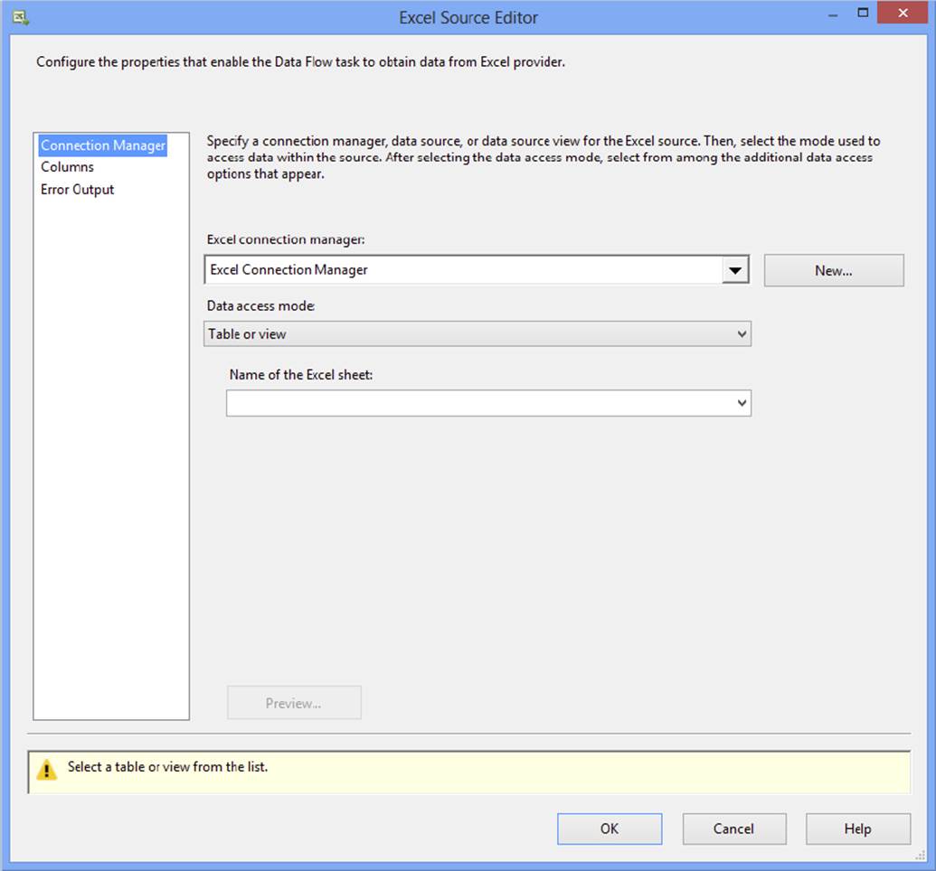

FIGURE 14-5

9. For this example the data access mode should be set to SQL Command because you only want to import rows with the physical count filled in. Type the following query (Excel_Import_SQL.txt) into the SQL command text box (see Figure 14-6):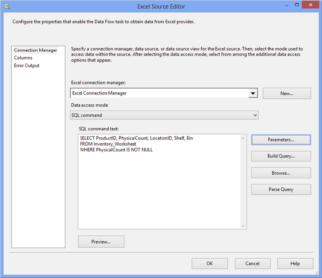

FIGURE 14-6

SELECT ProductID, PhysicalCount, LocationID, Shelf, Bin

FROM Inventory_Worksheet

WHERE PhysicalCount IS NOT NULL

10.Double-click the Inventory Import Component to bring up the OLE DB Destination Editor. Make sure the AdventureWorks connection is chosen. Under Data access mode, choose Table or View.

11.Click the New button next to Name of the table or the view to open the Create Table dialog.

12.Change the name of the table to InventoryImport and click OK to create the table. Select Mappings. Each field from the worksheet should match up to a field in the new table.

13.Click OK to accept the configuration.

While this is a simple example, it illustrates just how easy it is to import from and export to Excel files.

Importing from Excel 2007 and Later

Setting up an SSIS package to import from Excel 2007 and later is very similar to setting up the connection when exporting to Excel 2007.

When you set up the connection, choose Excel 2007 from the Excel version dropdown (step 5 above). Once you have set up the connection as already shown in Figures 14-5 and 14-6, you need to create an OLE DB Source adapter in the Data Flow. You can either reference the worksheet directly or specify a query that extracts data from specific Excel columns. Figure 14-7 shows a worksheet directly referenced, called “Inventory_Worksheet$.”

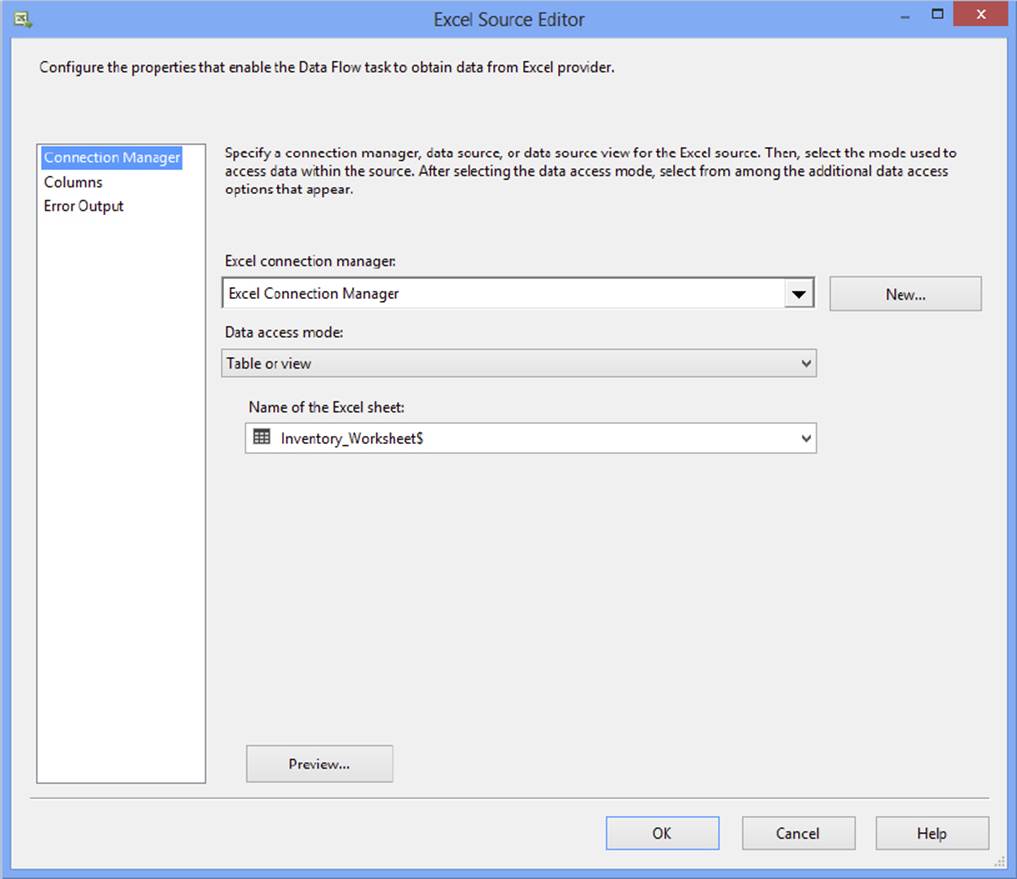
FIGURE 14-7

Working with Access

MS Access is the departmental database of choice for countless individual users and small workgroups. It has many great features and wizards that enable a small application or prototype to be quickly developed. Often, when an application has outgrown its humble Access origins, discussions about moving the data to SQL Server emerge. Many times, the client will be rewritten as a web or desktop application using VB.NET or another language. Sometimes the plan is to link to the SQL Server tables, utilizing the existing Access front end. Unfortunately, if the original application was poorly designed, moving the data to SQL Server will not improve performance. This section demonstrates how you can use SSIS to integrate with Microsoft Access. Access 2007 and later use the same ACE provider as Excel does, so as you work with Access in a 32-bit or 64-bit mode, please refer to the 64-bit discussion of Excel in the previous section.

Configuring an Access Connection Manager

Once the Connection Manager is configured properly, importing from Access is simple. First, look at the steps required to set up the Connection Manager:

1. Create a new SSIS package and create a new Connection Manager by right-clicking in the Connection Managers section of the design surface.

2. Select New OLE DB Connection to bring up the Configure OLE DB Connection Manager dialog.

3. Click New to open the Connection Manager. In the Provider dropdown list, choose one of the following access provider types:

· Microsoft Jet 4.0 OLE DB Provider (for Access 2003 and earlier)

· Microsoft Office 12.0 Access Database Engine OLE DB Provider (for Access 2007 and later)

If you do not see the Microsoft Office 12.0 Access Database Engine provider in the list, you need to install the 32-bit ACE driver described earlier.

4. Click OK after making your selection.

5. The Connection Manager dialog changes to an Access-specific dialog. In the server or file name box, enter the path to the Northwind database, C:\ProSSIS\Data\Northwind.mdb, as Figure 14-8 shows. You are using the Northwind MS Access sample database for this example.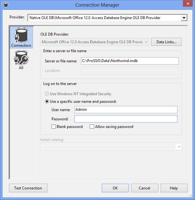

FIGURE 14-8

6. By default, the database user name is blank, with a blank password. If security has been enabled for the Access database, a valid user name and password must be entered. Enter the password on the All pane in the Security section. The user Password property is also available in the properties window. Check the Save my password option.

7. If, conversely, a database password has been set, enter the database password in the Password property on the Connection pane. This also sets the ODBC:Database Password property found on the All tab.

8. If both user security and a database password have been set up, enter both passwords on the All pane. In the Security section, enter the user password and the database password for the Jet OLEDB:New Database Password property. Check the Save my password option. Be sure to test the connection and click OK to save the properties.

Importing from Access

Once you have the Connection Manager created, follow these steps to import from Access:

1. Using the project you created in the last section with the Access Connection Manager already configured, add a Data Flow Task to the Control Flow design area.

2. Click the Data Flow tab to view the Data Flow design area. Add an OLE DB Source Component and name it Customers.

3. Double-click the Customers icon to open the OLE DB Source Editor. Set the OLE DB Connection Manager property to the Connection Manager that you created in the last section.

4. Select Table or View from the Data access mode dropdown list. Choose the Customers table from the list under Name of the table or the view (see Figure 14-9).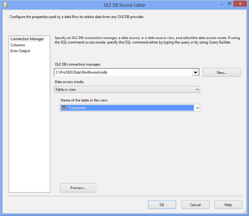

FIGURE 14-9

5. Click Columns on the left of the Source Editor to choose which columns to import and change the output names if needed.

6. Click OK to accept the configuration.

7. Create a Connection Manager pointing to AdventureWorks.

8. Create an OLE DB Destination Component and name it NW_Customers. Drag the connection (blue arrow on your screen) from the Customers Source Component to the NW_Customers Destination Component.

9. Double-click the Destination Component to bring up the OLE DB Destination Editor and configure it to use the AdventureWorks Connection Manager.

10.You can choose an existing table or you can click New to create a new table as the Data Destination. If you click New, notice that the Create Table designer does not script any keys, constraints, defaults, or indexes from Access. It makes its best guess as to the data types, which may not be the right ones for your solution. When building a package for use in a production system, you will probably want to design and create the SQL Server tables in advance.

11.For now, click New to bring up the table definition (see Figure 14-10). Notice that the table name is the same as the Destination Component, so change the name to NW_Customers if you did not name the OLE DB Destination as instructed previously.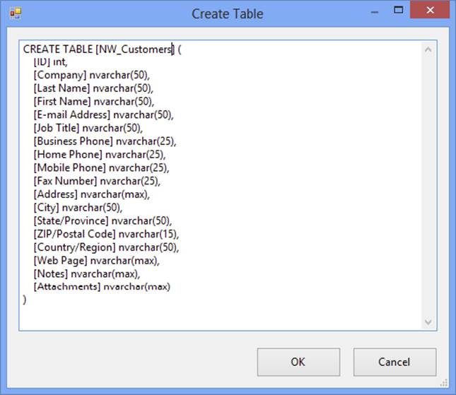

FIGURE 14-10

12.Click OK to create the new table.

13.Click Mappings on the left to map the source and destination columns.

14.Click OK to accept the configuration.

15.Run the package. All the Northwind customers should now be listed in the SQL Server table. Check this by clicking New Query in Microsoft SQL Server Management Studio. Run the following query (Access_Import.txt) to see the results:

16. USE AdventureWorks

17. GO

SELECT * FROM NW_Customers

18.Empty the table to prepare for the next example by running this query:

TRUNCATE TABLE NW_CUSTOMERS

Using a Parameter

Another interesting feature is the capability to pass a parameter from a package variable to a SQL command. The following steps demonstrate how:

NOTE In Access, you can create a query that prompts the user for parameters at runtime. You can import most Access select queries as tables, but data from an Access parameter query cannot be imported using SSIS.

1. Select the package you started in the last section.

2. Navigate back to the Control Flow tab and right-click the design area.

3. Choose Variables and add a variable by clicking the Add Variable icon. Name it CustomerID. Change the Data Type to String, and give it a value of ANTON (see Figure 14-11). Close the Variables window and navigate back to the Data Flow tab.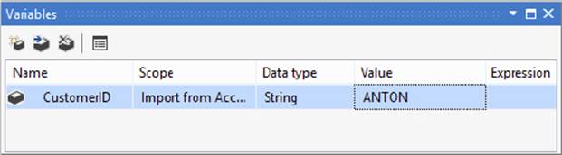

FIGURE 14-11

NOTE The design area or component that is selected determines the scope of the variable when it is created. The scope can be set to the package if it is created right after clicking the Control Flow design area. You can also set the scope to a Control Flow Task, Data Flow Component, or Event Handler Task.

4. Double-click the Customers Component to bring up the OLE DB Source Editor and change the data access mode to SQL Command. A SQL Command text box and some buttons appear. You can click the Build Query button to bring up a designer to help build the command or click Browse to open a file with the command you want to use. For this example, type in the following SQL statement (Access_Import_Parameter.txt) (see Figure 14-12):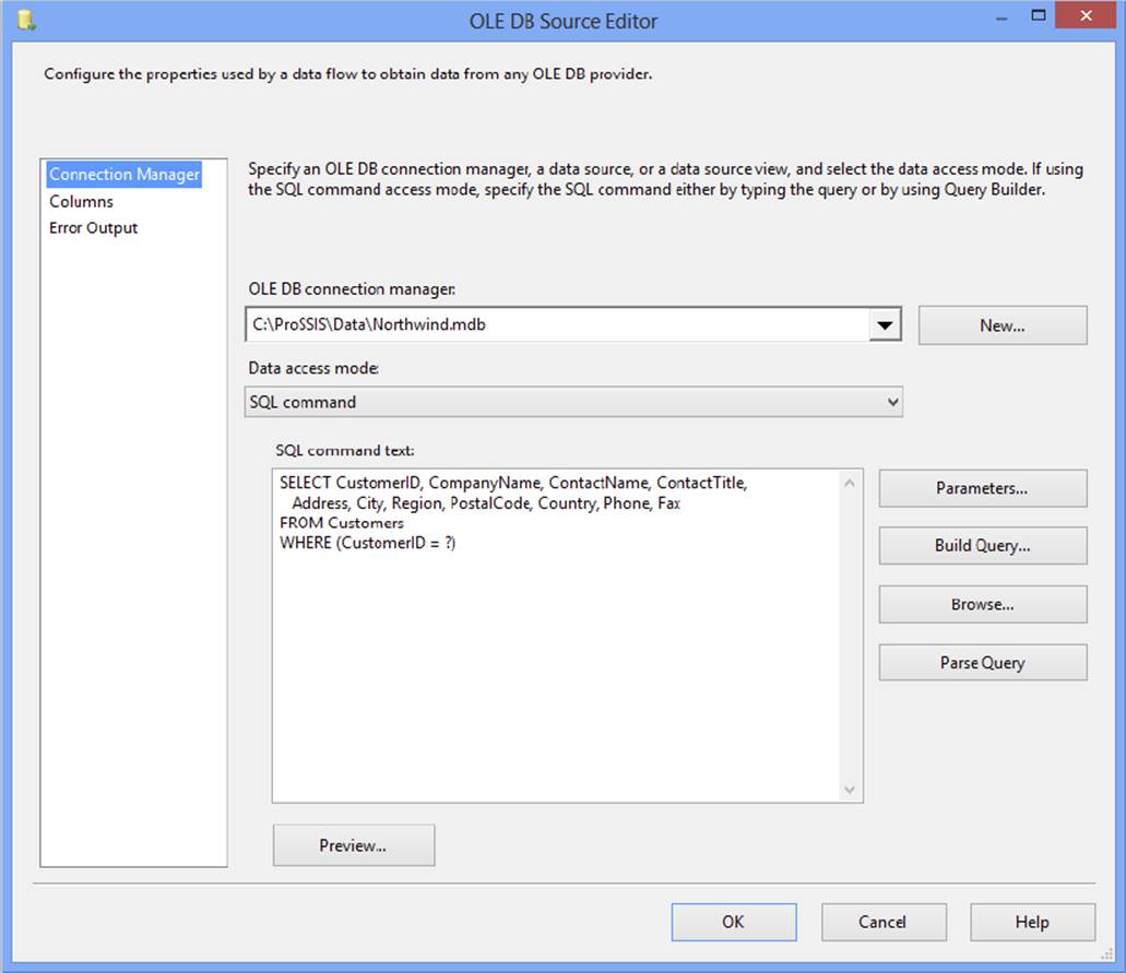

FIGURE 14-12

SELECT CustomerID, CompanyName, ContactName, ContactTitle,

Address, City, Region, PostalCode, Country, Phone, Fax

FROM Customers

WHERE (CustomerID = ?)

5. The ? symbol is used as the placeholder for the parameter in the query. Map the parameters to variables in the package by clicking the Parameters button. Choose User::CustomerID from the Variables list and click OK (see Figure 14-13).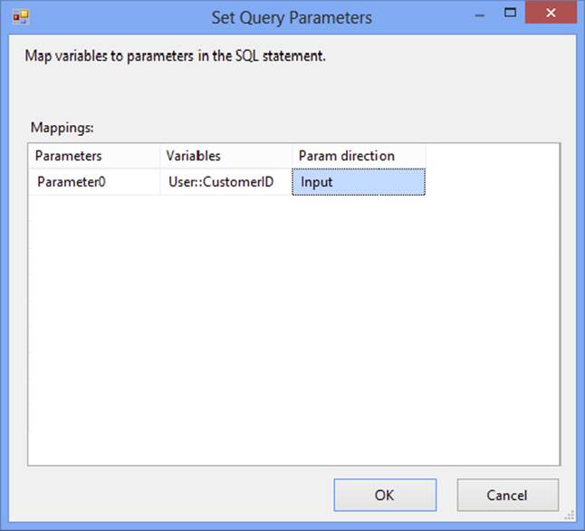

FIGURE 14-13

Note that you cannot preview the data after setting up the parameter because the package must be running to load the value into the parameter.

NOTE Variables in SSIS belong to namespaces. By default, there are two namespaces, User and System. Variables that you create belong to the User namespace. You can also create additional namespaces.

6. Click OK to accept the new configuration and run the package. This time, only one record is imported (see Figure 14-14).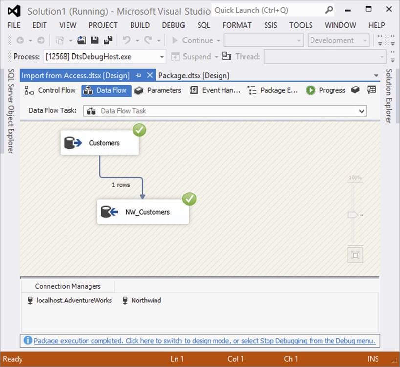

FIGURE 14-14

You can also return to SQL Server Management Studio to view the results:

USE AdventureWorks

SELECT * FROM NW_Customers

If you wish to use multiple parameters in your SQL command, use multiple question marks (?) in the query and map them in order to the parameters in the parameter mapping. To do this, you set up a second package-level variable for CompanyName and set the value to Island Trading. Change the query in the Customers Component to the following (Access_Import_Parameter2.txt):

SELECT CustomerID, CompanyName,

ContactName, ContactTitle, Address, City, Region,

PostalCode, Country, Phone, Fax

FROM Customers

WHERE (CustomerID = ?) OR

(CompanyName = ?)

Now the Parameters dialog will show the two parameters. Associate each parameter with the appropriate variable (see Figure 14-15).

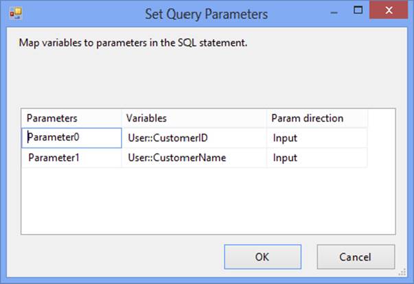
FIGURE 14-15

Importing data from Access is a simple process as long as Access security has not been enabled. Often, porting an Access application to SQL Server is the desired result. Make sure you have a good book or other resource to help ensure success.

IMPORTING FROM ORACLE

Because of SQL Server’s world-class reporting and business intelligence tools, more and more shops running Oracle rely on SQL Server for their reporting needs.

Luckily, importing data from Oracle is much like importing from other sources, such as a text file or another SQL Server instance. In this section, you learn how to access data from an Oracle database with the built-in OLE DB provider and the Oracle client.

Oracle Client Setup

Connecting to Oracle in SSIS is a two-step process. First you install the Oracle client software, and then you use the OLE DB provider in SSIS to connect to Oracle.

To be sure, the Microsoft Data Access Components (MDAC) that comes with the operating system include an OLE DB provider for Oracle. This is the 32-bit Microsoft-written OLE DB provider to access an Oracle source system. However, even though the OLE DB provider is installed, you cannot use it until you install a second component, the Oracle client software. In fact, when you install the Oracle client software, Oracle includes an OLE DB provider that can be used to access an Oracle source. The OLE DB providers have subtle differences, which are referenced later in this section.

Installing the Oracle Client Software

To install the Oracle client software, you first need to locate the right download from the Oracle website at www.oracle.com. Click Downloads and then click the button to download 12c. Accept the licensing agreement and select your operating system. As you are well aware, there are several versions of Oracle (currently Oracle 11g, 11g Release 2, 12c), and each has a different version of the Oracle client. Some of them are backward compatible, but it is always best to go with the version that you are connecting to.

It is best to install the full client software in order to ensure that you have the right components needed for the OLE DB providers.

Configuring the Oracle Client Software

Once you download and install the right client for the version of Oracle you will be connecting to and the right platform of Windows you are running, the final step is configuring it to reference the Oracle servers. You will probably need help from your Oracle DBA or the support team of the Oracle application to configure this.

There are two options: an Oracle name server or manually configuring a TNS file. The TNS file is more common and is found in the Oracle install directory under the network\ADMIN folder. This is called the Oracle Home directory. The Oracle client uses the Windows environment variables %Path% and %ORACLE_HOME% to find the location to the client files. Either replace the default TNS file with one provided by an Oracle admin or create a new entry in it to connect to the Oracle server.

A typical TNS entry looks like this:

[Reference name] =

(DESCRIPTION =

(ADDRESS_LIST = (ADDRESS = (PROTOCOL = TCP)

(HOST = [Server])(PORT = [Port Number])) )

(CONNECT_DATA =

(SID = [Oracle SID Name])

)

Replace the brackets with valid entries. The [Reference Name] will be used in SSIS to connect to the Oracle server through the provider.

64-Bit Considerations

As mentioned earlier, after you install the Oracle client software, you can then use the OLE DB provider for Oracle in SSIS to extract data from an Oracle source or to send data to an Oracle Destination. These procedures are described next. However, if you are working on a 64-bit server, you may need to make some additional configurations.

First, if you want to connect to Oracle with a native 64-bit connection, you have to use the Oracle-written OLE DB provider for Oracle because the Microsoft-written OLE DB driver for Oracle is available only in a 32-bit mode. Be sure you also install the right 64-bit Oracle client (Itanium IA64 or X64) if you want to connect to Oracle in native 64-bit mode. Although it is probably obvious to you, it bears mentioning that even though you may have X64 hardware, in order to leverage it in 64-bit mode, the operating system must be installed with the X64 version.

Furthermore, even though you may be working on a 64-bit server, you can still use the 32-bit provider through the 32-bit Windows emulation mode. Review the 64-bit details in the “Excel and Access” section earlier in this chapter for details about how to work with packages in 32-bit mode when you are on a 64-bit machine. You need to use the 32-bit version of DTExec for package execution, and when working in SSDT, you need to change the Run64bitRuntime property of the project to False.

Importing Oracle Data

In this example, the alias ORCL is used to connect to an Oracle database named orcl. Your Oracle administrator can provide more information about how to set up your tnsnames.ora file to point to a test or production database in your environment. The followingtnsnames file entry is being used for the subsequent steps:

ORCL =

(DESCRIPTION =

(ADDRESS = (PROTOCOL = TCP)(HOST = VPC-XP)(PORT = 1521))

(CONNECT_DATA =

(SERVER = DEDICATED) (SERVICE_NAME = orcl)

)

To extract data from an Oracle server, perform the following steps. These assume that you have installed the Oracle client and configured a tnsnames file or an Oracle names server.

1. Create a new Integration Services project using SSDT.

2. Add a Data Flow Task to the design area. On the Data Flow tab, add an OLE DB source. Name the OLE DB source Oracle.

3. In the Connection Managers area, right-click and choose New OLE DB Connection to open the Configure OLE DB Connection Manager dialog.

4. Click New to open the Connection Manager dialog. Select Microsoft OLE DB Provider for Oracle from the list of providers and click OK.

5. Type the alias from your tnsnames.ora file for the Server Name.

6. Type in the user name and password and check Save my password (see Figure 14-16). This example illustrates connecting to the widely available scott sample database schema. The user name is scott; the password is tiger. Verify the credentials with your Oracle administrator. Test the connection to ensure that everything is configured properly. Click OK to accept the configuration.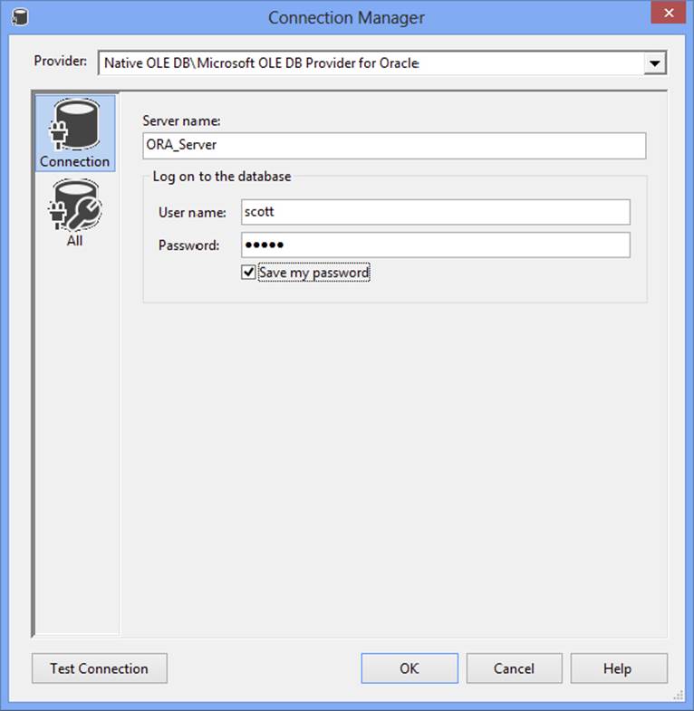

FIGURE 14-16

7. In the custom properties section of the Oracle Component’s property dialog, change the AlwaysUseDefaultCodePage property to True.

8. Open the OLE DB Source Editor by double-clicking the Oracle Source Component. With the Connection Manager tab selected, choose the Connection Manager pointing to the Oracle database.

9. Select Table or view from the Data access mode dropdown. Click the dropdown list under Name of the table or the view to see a list of the available tables. Choose the “Scott”.“Dept” table from the list.

10.Select the Columns tab to see a list of the columns in the table.

11.Click Preview to see sample data from the Oracle table. At this point, you can add a Data Destination Component to import the data into SQL Server or another OLE DB Destination. This is demonstrated several times elsewhere in the chapter, so it isn’t covered again here.

Importing Oracle data is very straightforward, but there are a few things to watch out for. The current Microsoft ODBC driver and Microsoft-written OLE DB provider for Oracle were designed for Oracle 7. At the time of this writing, Oracle 11g is the latest version available. Specific functionality and data types that were implemented after the 7 release will probably not work as expected. See Microsoft’s Knowledge Base article 244661 for more information. If you want to take advantage of newer Oracle features, you should consider using the Oracle-written OLE DB provider for Oracle, which is installed with the Oracle client software.

USING XML AND WEB SERVICES

Although XML is not a common source for large volumes of data, it is an integral technology standard in the realm of data. This section considers XML from a couple of different perspectives. First, you will work with the Web Service Task to interact with a public web service. Second, you will use the XML Source adapter to extract data from an XML document embedded in a file. In one of the web service examples, you will also use the XML Task to read the XML file.

Configuring the Web Service Task

In very simple terms, a web service is to the web as a function is to a code module. It accepts a message in XML, including arguments, and returns the answer in XML. The value of XML technology is that it enables computer systems that are completely foreign to each other to communicate in a common language. When using web services, this transfer of XML data occurs across the enterprise or across the Internet using the HTTP protocol. Many web services — for example, stock-tickers and movie listings — are freely available for anyone’s use. Some web services, of course, are private or require a fee. Two common and useful applications are to enable orders or other data to be exchanged easily by corporate partners, and to receive information from a service — either one that you pay for or a public service that is exposed free on the Internet. In the following examples, you’ll learn how to use a web service to get the weather forecast of a U.S. zip code by subscribing to a public web service, and how to use the Web Service Task to perform currency conversion. Keep in mind that the web service task depends on the availability of a server. The Web Service Task could return errors if the server is unreachable or if the server is experiencing any internal errors.

Weather by Zip Code Example

This example demonstrates how to use a web service to retrieve data:

1. Create a new package and create an HTTP Connection by right-clicking in the Connection Managers pane and choosing New Connection.

2. Choose HTTP and click Add to bring up the HTTP Connection Manager Editor. Type http://www.webservicex.net/WeatherForecast.asmx?wsdl as the Server URL (see Figure 14-17). In this case, you’ll use a publicly available web service, so you won’t have to worry about any credentials or certificates. If you must supply proxy information to browse the web, fill that in on the Proxy tab.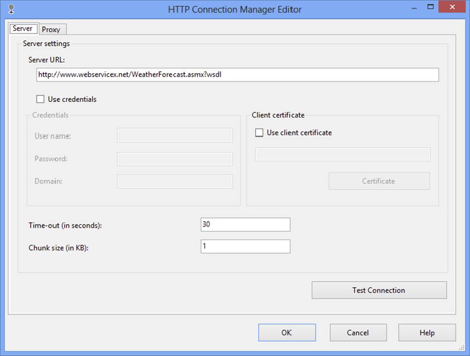

FIGURE 14-17

3. Before continuing, click the Test Connection button, and then click OK to accept the Connection Manager.

4. Add a Web Service Task from the Toolbox to the Control Flow workspace.

5. Double-click the Web Service Task to bring up the Web Service Task Editor. Select the General pane. Make sure that the HttpConnection property is set to the HTTP connection you created in step number 2.

6. In order for a web service to be accessed by a client, a Web Service Definition Language (WSDL) file must be available that describes how the web service works — that is, the methods available and the parameters that the web service expects. The Web Service Task provides a way to automatically download this file.

7. In the WSDLFile property, enter the fully qualified path c:\ProSSIS\Data\weather.wsdl where you want the WSDL file to be created (see Figure 14-18).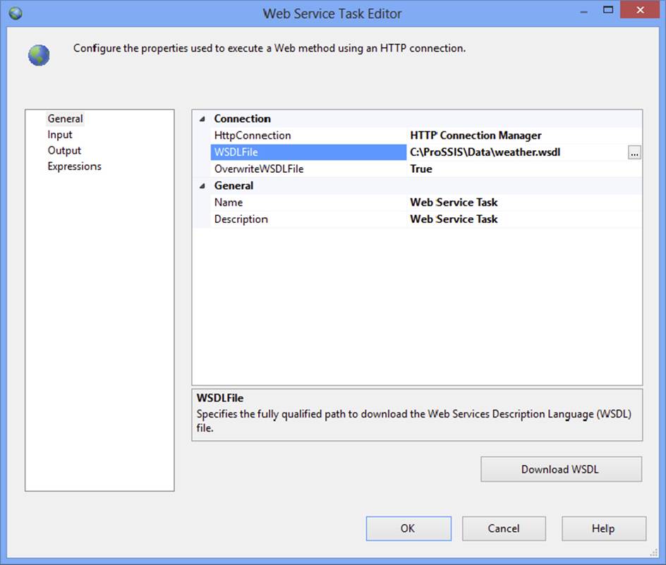

FIGURE 14-18

8. Set the OverwriteWSDLFile property to True and then click Download WSDL to create the file. If you are interested in learning more about the file’s XML structure, you can open it with Internet Explorer.

By downloading the WSDL file, the Web Service Task now knows the web service definition.

9. Select the Input pane of the Web Service Task Editor. Then, next to the Service property, open the dropdown list and select the one service provided, called WeatherForecast.

10.After selecting the WeatherForecast service, click in the Method property and choose the GetWeatherByZipCode option.

11.Web services are not limited to providing just one method. If multiple methods are provided, you’ll see all of them listed. Notice another option called GetWeatherByPlaceName. You would use this if you wanted to enter a city instead of a zip code. Once the GetWeatherByZipCode method is selected, a list of arguments appears. In this case, a ZipCode property is presented. Enter a zip code location of a U.S. city (such as 30303 for Atlanta, or, if you live in the U.S., your own zip code). See Figure 14-19.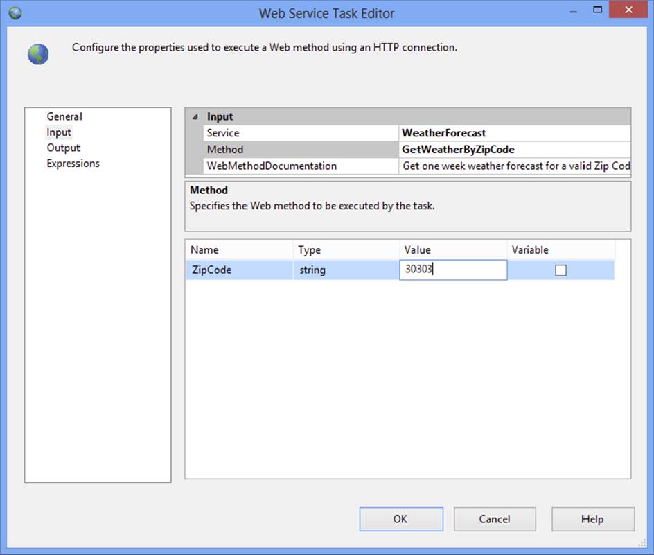

FIGURE 14-19

12.Now that everything is set up to invoke the web service, you need to tell the Web Service Task what to do with the result. Switch to the Output property page of the Web Service Task Editor. Choose File Connection in the dropdown of the OutputType property. You can also store the output in a variable to be referenced later in the package.

13.In the File property, open the dropdown list and choose <new connection>.

14.When you are presented with the File Connection Manager Editor, change the Usage type property to Create file and change the File property to C:\ProSSIS\Data\weatheroutput.xml, as shown in Figure 14-20.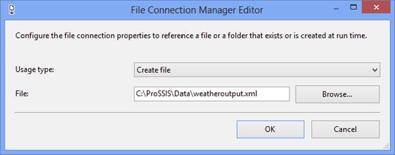

FIGURE 14-20

15.Select OK in the File Connection Manager Editor, and OK in the Web Service Task Editor to finish configuring the SSIS package.

Now you’re ready to run the package. After executing it, wait for the Web Service Task to complete successfully. If all went well, use Internet Explorer to open the XML file returned by the web service (c:\ProSSIS\data\weatheroutput.xml) and view the weather forecast for the zip code. It will look something like this:

<?xml version="1.0" encoding="utf-16" ?>

<WeatherForecasts xmlns:xsi=http://www.w3.org/2001/XMLSchema-instance

xmlns:xsd="http://www.w3.org/2001/XMLSchema">

<PlaceName xmlns="http://www.webservicex.net">ATLANTA</PlaceName>

<Day>Thursday, September 01, 2011</Day>

<WeatherImage>http://forecast.weather.gov/images/wtf/nfew.jpg</WeatherImage>

</WeatherData>

<Day>Friday, September 02, 2011</Day>

</Details>

</WeatherForecasts>

The Currency Conversion Example

In this second example, you learn how to use a web service to get a value that can be used in the package to perform a calculation. To convert a price list to another currency, you’ll use the value with the Derived Column Transformation:

1. Begin by creating a new SSIS package. This example requires three variables. To set them up, ensure that the Control Flow tab is selected. If the Variables window is not visible, right-click in the design area and select Variables. Set up the three variables as shown in the following table. At this time, you don’t need initial values. (You can also use package parameters instead of variables for this example.)

NAME	SCOPE	DATA TYPE
XMLAnswer	Package	String
Answer	Package	String
ConversionRate	Package	Double

2. Add a Connection Manager pointing to the AdventureWorks database.

3. Add a second connection. This time, create an HTTP Connection Manager and set the Server URL to http://www.webservicex.net/CurrencyConvertor.asmx?wsdl.

NOTE Note that this web service was valid at the time of publication, but the authors cannot guarantee its future availability.

4. Drag a Web Service Task to the design area and double-click the task to open the Web Service Task Editor. Set the HTTPConnection property to the Connection Manager you just created.

5. Type in a location to store the WSDLFile, such as c:\ProSSIS\data\CurrencyConversion.wsdl, and then click the Download WSDL button as you did in the last example to download the WSDL file.

6. Click Input to see the web service properties. Select CurrencyConvertor as the Service property and ConversionRate as the Method.

7. Two parameters will be displayed: FromCurrency and ToCurrency. Set FromCurrency equal to USD, and ToCurrency equal to EUR (see Figure 14-21).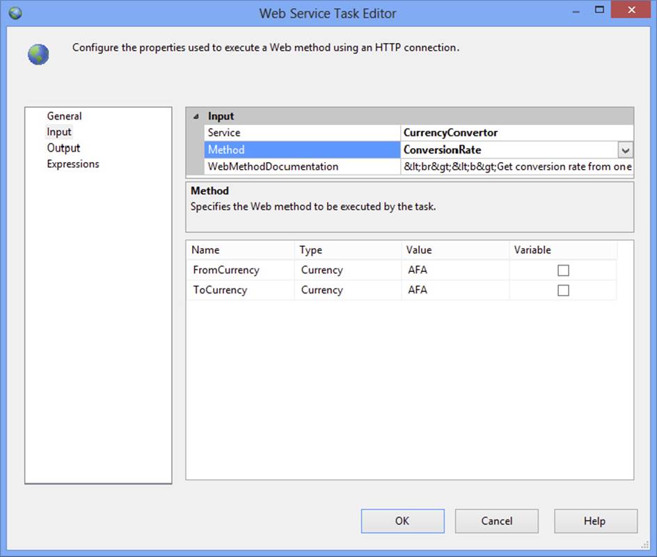

FIGURE 14-21

8. Click Output and set the OutputType to Variable.

9. The variable name to use is User::XMLAnswer (see Figure 14-22). Click OK to accept the configuration.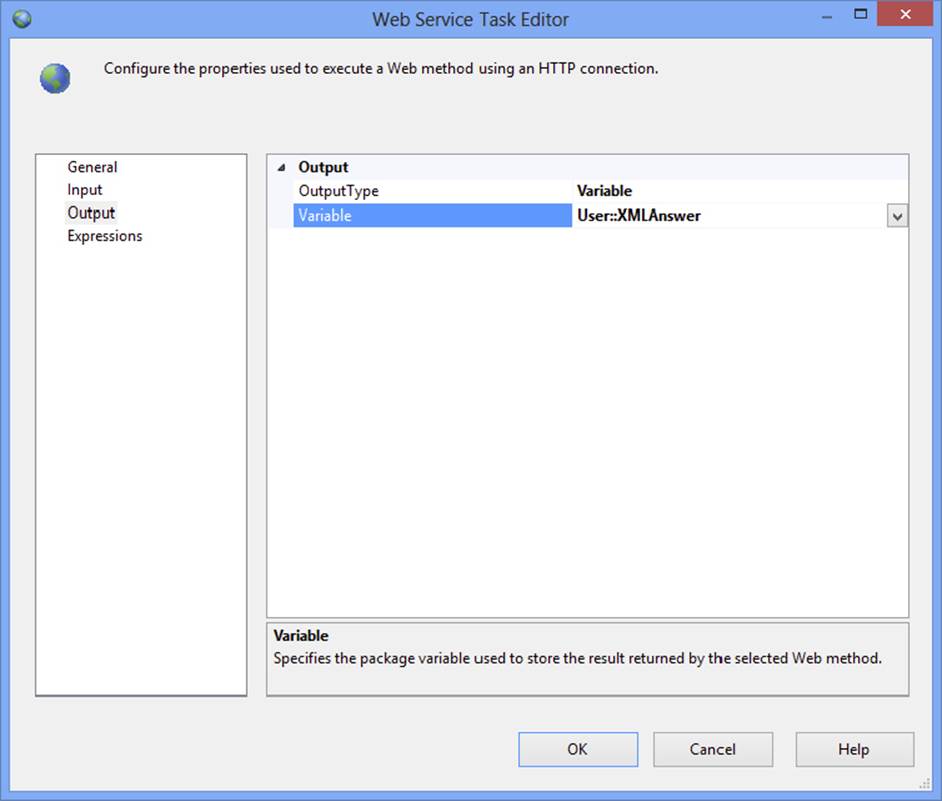

FIGURE 14-22

NOTE At this point, you may be interested in viewing the XML that it returned from the web service. You can save the XML in a file instead of a variable. Then, after running the task, examine the file. Alternately, you can set a breakpoint on the task and view the variable at runtime. See Chapter 18 to learn more about breakpoints and debugging.

The value of the XML returned will look something like this:

<?xml version="1.0" encoding="utf-8">

10.Because (for the sake of the example) you just need the number and not the XML, add an XML Task to the designer to evaluate the XML.

11.Drag the precedence constraint from the Web Service Task to the XML Task, and then open the XML Task Editor by double-clicking the XML Task.

12.Change the OperationType to XPATH. The properties available will change to include those specific for the XPATH operation. Set the properties to match those in the following table:

SECTION	PROPERTY	VALUE
Input	OperationType	XPATH
	SourceType	Variable
	Source	User:XMLAnswer
Output	SaveOperationResult	True
Operation Result	OverwriteDestination	True
	Destination	User::Answer
	DestinationType	Variable
Second Operand	SecondOperandType	Direct Input
	SecondOperand	/
Xpath Options	PutResultInOneNode	False
	XpathOperation	Values

A discussion about the XPATH query language is beyond the scope of this book, but this XML is very simple with only a root element that can be accessed by using the slash character (/). Values are returned from the query as a list with a one-character unprintable row delimiter. In this case, only one value is returned, but it still has the row delimiter that you can’t use.

You have a couple of options here. You could save the value to a file, then import using a File Source Component into a SQL Server table, and finally use the Execute SQL Task to assign the value to a variable; but in this example, you will get a chance to use the Script Task to eliminate the extra character:

1. Add a Script Task to the design area and drag the precedence constraint from the XML Task to the Script Task.

2. Open the Script Task Editor and select the Script pane.

3. In order for the Script Task to access the package variables, they must be listed in the ReadOnlyVariables or ReadWriteVariables properties (as appropriate considering whether you will be updating the variable value in the script) in a semicolon-delimited list. Enter User::Answer in the ReadOnlyVariables property and User::ConversionRate in the ReadWriteVariables property (see Figure 14-23).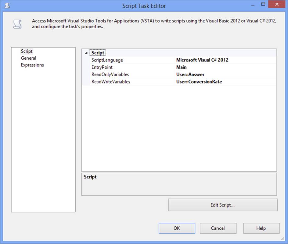

FIGURE 14-23

4. Click Design Script to open the code window. A Microsoft Visual Studio Tools for Applications environment opens. The script will save the value returned from the web service call to a variable. One character will be removed from the end of the value, leaving only the conversion factor. This is then converted to a double and saved in the ConversionRate variable for use in a later step.

5. Replace Sub Main with the following code (Currency_Script.txt):

6. Public Sub Main()

7. Dim strConversion As String

8. strConversion = Dts.Variables("User::Answer").Value.ToString

9. strConversion = strConversion.Remove(strConversion.Length -1,1)

10. Dts.Variables("User::ConversionRate").Value = CType(strConversion,Double)

11. Dts.TaskResult = Dts.Results.Success

End Sub

12.Close the scripting environment, and then click OK to accept the Script Task configuration.

13.Add a Data Flow Task to the design area and connect the Script Task to the Data Flow Task. The Control Flow area should resemble what is shown in Figure 14-24.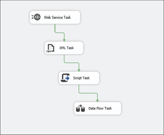

FIGURE 14-24

14.Move to the Data Flow tab and add a Connection Manager pointing to the AdventureWorks database, if you did not do so when getting started with this example.

15.Drag an OLE DB Source Component to the design area.

16.Open the OLE DB Source Editor and set the OLE DB Connection Manager property to the AdventureWorks connection. Change the data access mode property to SQL Command. Type the following query (Currency_Select.txt) in the command window:

17. SELECT ProductID, ListPrice

18. FROM Production.Product

WHERE ListPrice> 0

19.Click OK to accept the properties.

20.Add a Derived Column Transformation to the design area.

21.Drag the Data Flow Path from the OLE DB Source to the Derived Column Component.

22.Double-click to open the Derived Column Transformation Editor dialog. Variables, columns, and functions are available for easily building an expression. Add a derived column called EuroListPrice. In the Expression field, type the following (Currency_Expression.txt):

ListPrice * @[User::ConversionRate]

23.The Data Type should be a decimal with a scale of 2. Click OK to accept the properties (see Figure 14-25).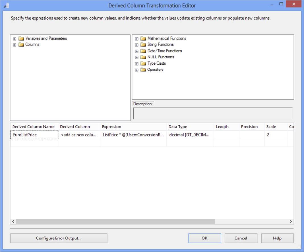

FIGURE 14-25

24.Add a Flat File Destination Component to the Data Flow design area. Drag the Data Flow Path from the Derived Column Component to the Flat File Destination Component.

25.Bring up the Flat File Destination Editor and click New to open the Flat File Format dialog.

26.Choose Delimited and click OK. The Flat File Connection Manager Editor will open.

27.Browse to or type in the path to a file, C:\ProSSIS\data\USD_EUR.txt. Here you can modify the file format and other properties if required (see Figure 14-26). Check Column names in the first data row.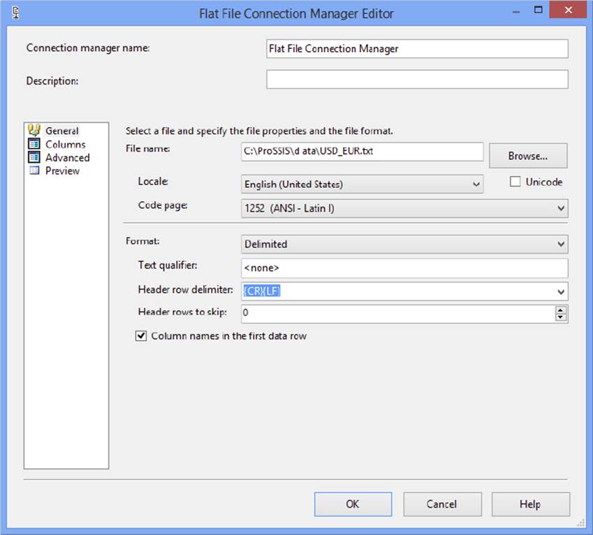

FIGURE 14-26

28.Click OK to dismiss the Flat File Connection Manager Editor dialog and return to the Flat File Destination Editor.

29.Click Mappings and then click OK.

30.Run the package and then open the file that was created by the destination adapter, C:\ProSSIS\data\USD_EUR.txt. You should see a list of products along with the list price and the list price converted to euros.

Many web services are available for you to try. See www.xmethods.net for a list of services, some of which are free. In the next section, you learn how to import an XML file into relational tables.

Working with XML Data as a Source

SQL Server provides many ways to work with XML. The XML Source adapter is yet another jewel in the SSIS treasure chest. It enables you to import an XML file directly into relational tables if that is what you need. In this example, you import an RSS (Really Simple Syndication) file from the web.

To use the XML Source adapter in SSIS, you first connect to an XML file, and then you need to provide the XSD definition of the XML structure, so that SSIS can read the file and correctly interpret the XML elements and attribute structure. Don’t have an XSD? No problem; SSIS can self-generate the XSD from within the XML Source adapter. There is no guarantee that the generated XSD will work with another XML file coming from the same source, which is why it is better to have an XSD definition that is provided by the XML Source that will universally apply to the related files used by SSIS.

1. Create a new Integration Services package to get started.

2. Add a Data Flow Task to the Control Flow design area and then click the Data Flow tab to view the Data Flow design area.

3. Add an XML Source and name it CD Collection.

4. Double-click the CD Collection Component to open the XML Source Editor.

5. Make sure that the Connections Manager property page is selected on the left.

6. Select XML File Location for the data access mode. For the XML location property, type in the following address:

C:\ProSSIS\Data\cd_catalog.xml

If you click the Browse button, a regular File Open dialog opens. It isn’t obvious at first that you can use a URL instead of a file on disk.

The XML file must be defined with an XML Schema Definition (XSD), which describes the elements in the XML file. Some XML files have an in-line XSD, which you can determine by opening the file and looking for xsd tags. There are many resources and tutorials available on the web if you want to learn more about XML schemas. If the file you are importing has an in-line schema, make sure that Use inline schema is checked. If an XSD file is available, you can enter the path in the XSD location property (seeFigure 14-27). In this case, you will create the XSD file right in the Source adapter.

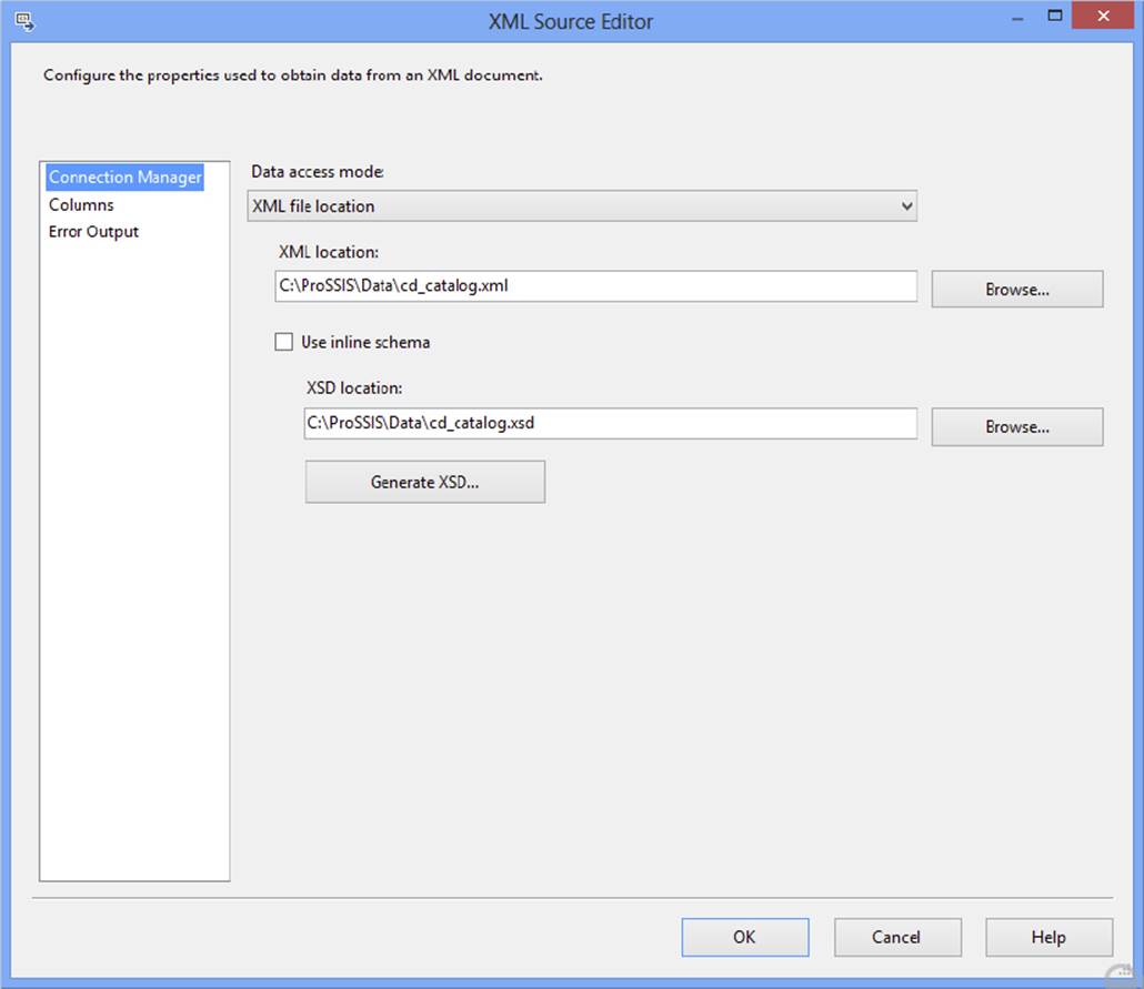
FIGURE 14-27

7. Click Generate XSD and put the file in a directory on your machine (such as c:\ProSSIS\data\cd_catalog.xsd). Once the file is generated, you can open it with Internet Explorer to view it if you are interested in learning more.

8. Now that the CD Collection Component understands the XML file, click Columns. You will see all the columns defined in the XML file, as Figure 14-28 shows.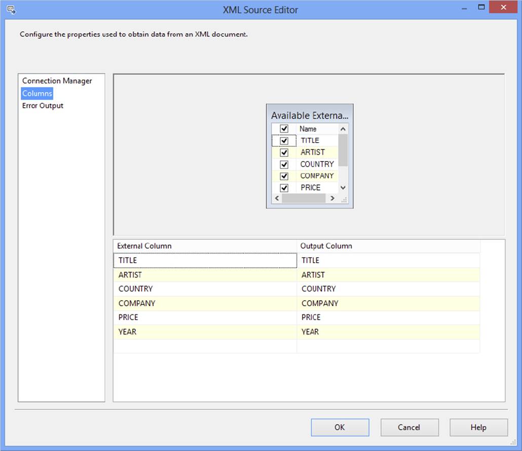

FIGURE 14-28

Even though the XML document is one file, it represents two tables with a one-to-many relationship. If you browse to C:\ProSSIS\Data\cd_catalog.xml, you’ll see a channel, which describes the source of the information, usually news, and several items, or articles, defined. One note of caution here: if you are importing into tables with primary/foreign key constraints, there is no guarantee that the parent rows will be inserted before the child rows. Be sure to keep that in mind as you design your XML solution.

The properties of the channel and item tags match the columns displayed in the XML Source Editor. At this point, you can choose which fields you are interested in importing and change the output names if required. When you use the XML Source adapter, all the output name selections will be available as downstream paths. When you use an output path from the XML Source adapter, you will be able to choose which output you want to use.

1. Create a new Connection Manager pointing to the AdventureWorks database or another test database.

2. Add an OLE DB Destination Component to the design area and name it CD Collection _Table.

3. Drag the Data Flow Path (blue arrow on the screen) from the XML Source to CD Collection Table.

4. Double-click the CD Collection Table icon to bring up the OLE DB Destination Editor. Make sure that the OLE DB Connection Manager property is set to point to your sample database.

5. Next to Use Table or View, click New. A window with a table definition will pop up. Click OK to create the table. Click Mappings and then click OK to accept the configuration.

6. Add another OLE DB Destination Component and name it Errors. Drag a red Data Flow Path from the XML Source to the Errors Component. Click OK. The Configure Error Output dialog will open.

7. In the Truncation property of the Description row, change the value to Redirect row (see Figure 14-29) and click OK.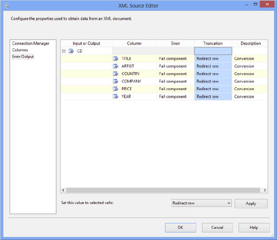

FIGURE 14-29

8. Double-click the OLE DB Destination that you named Errors and make sure it is pointing to the test database. Click New next to “Name of the table or the view,” and then click OK to create an Errors table. Click Mappings to accept the mappings, and then click OK to save the configuration. The Data Flow design area should now resemble Figure 14-30.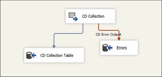

FIGURE 14-30

Run the package. If it completed successfully, some of the rows will be added to the NewsItem table. Any row with a description that exceeds 2,000 characters will end up in the Errors table.

FLAT FILES

Flat files are one of the more common sources to work with because data in the flat files is easy to read and create by most RDBMS systems and ETL tools. The challenges in working with flat files deal with handling data in a format in which data types are not enforced, and data that is structured in challenging ways. You may also run into files that are encoded into a different code page than ASCII, such as a UNIX encoding.

SSIS can handle various formats of flat files with varying code pages. The only challenging data is unstructured data, but this can also be handled in SSIS — not with the Flat File Source adapter but rather through a Script Component that is acting as a source. Refer to Chapter 9 for a primer on using the Script Component.

Loading Flat Files

Loading flat files from SSIS is a lot more straightforward than extracting data from a flat file. That’s because when you are loading data into a flat file from an SSIS Data Flow, SSIS already knows the specific data types and column lengths. Extracting data is harder because flat files do not contain information about the data types of the column or the structure of the file. This first example demonstrates how to use SSIS to create and load a flat file:

1. Create a new SSIS package with a Data Flow Task.

2. From the Toolbox, drag an OLE DB Source adapter onto the Data Flow and configure it to connect to the AdventureWorks database.

3. Change the data access mode to SQL Command and type the following SQL statement (Flat_File_Select.txt) in the text window:

4. SELECT Name, ProductNumber, ListPrice

FROM [Production].[Product]

5. Switch to the Columns property page of the OLE DB Source Editor and change the column selection to include only ProductID, Name, ProductNumber, ListPrice, and Size (these should be the only columns that are checked).

6. Select OK to save your changes to the OLE DB Source adapter.

7. Add a Flat File Destination adapter to the Data Flow (be sure to use the Flat File Destination and not the Source!) and connect the blue data path from the OLE DB Source to the Flat File Destination.

8. Double-click the Flat File Destination to open the editor.

9. Select New next to the Flat File Connection Manager dropdown, which opens a new window named Flat File Format (see Figure 14-31). Choose Fixed Width and select OK, which opens the Flat File Connection Manager Editor.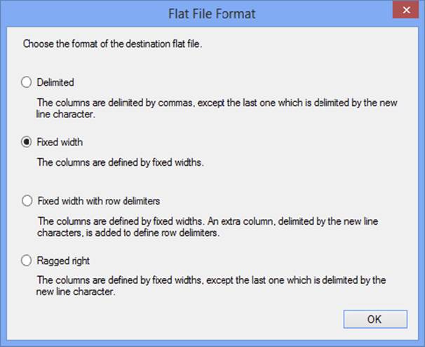

FIGURE 14-31

Creating and configuring a Flat File Connection Manager is easier to create from within a Destination adapter that already understands the data than by adding a Flat File Connection Manager directly in the Connection Manager window.

As Figure 14-31 shows, there are several options for the format of the flat file. The options for the flat file are described right in the selection window.

10.At this point, in the Flat File Connection Manager Editor, name your connection Products Flat File Destination, and pick a location and name for your file and enter it in the Filename window, such as c:\ProSSIS\data\products.txt.

11.Open the Code Page dropdown list and observe the dozens of supported code pages — from ANSI 1252 to IBM EBCDIC to UTF to MAC. Any of these can be selected if you intend to send the file to another machine that will consume the data in a different format. Change the Code page to 65001 (UTF-8), which should be the last one on the list.

12.Switch to the Advanced property page on the left, which displays a list of the columns that the Flat File Destination adapter received from the upstream transformation (in this case the Source adapter). Select OK to save the Flat File Connection Manager properties.

13.Finally, in the Flat File Destination Editor, click the Mappings property page on the left, which by default maps the input columns to the columns created in the destination file.

Note that in the Flat File Destination Editor, on the Connection Manager tab, there is a checkbox called “Overwrite data in the file” as Figure 14-32 shows. When this is checked, the file will be cleared before data is loaded in the Data Flow. If this is unchecked, then data will be appended to the file.

FIGURE 14-32

14.Leave “Overwrite data in the file” checked and select OK to save the Flat File Destination properties.

15.Run this simple package, which will create the flat file and overwrite any data that previously existed.

Extracting Data from Flat Files

Now that you have created and loaded a flat file, the next task is to understand how to extract data from a flat file. Of course, when you are working in your work environment, the first step in extracting data from a flat file is to make sure you have access to the file and you somewhat understand how the data is structured.

In this example, you will be working with a fixed-width file created in the prior example, encoded in UTF-8 code page format. The file contains a list of AdventureWorks products.

1. Create a new SSIS package and a new Data Flow Task within the package.

2. Drag the Flat File Source adapter from the Toolbox onto the Data Flow workspace and then double-click the Flat File Source to open the Flat File Source Editor.

3. Connecting to a flat file requires using a package connection. Therefore, in the Flat File Source Editor, click the New button next to the Flat File Connection Manager dropdown, which opens the Flat File Connection Manager Editor.

4. Name the connection Products File Source in the Connection manager name text box.

5. Click the Browse button and find the products.txt file that you created in the last exercise (such as c:\ProSSIS\data\products.txt).

6. Change the Code page to 65001 (UTF-8).

7. Change the Format dropdown to the Fixed-width selection option, and be sure to uncheck the option Column names in the first data row.

8. Switch to the Columns property page and note that because this file is a fixed-width file, you need to set the column widths. Click on the red vertical line and drag it to the right until the fields line up based on rows and columns, as Figure 14-33 shows (it is easier if your window is maximized, and alternately, you can just change the Row width property to 97).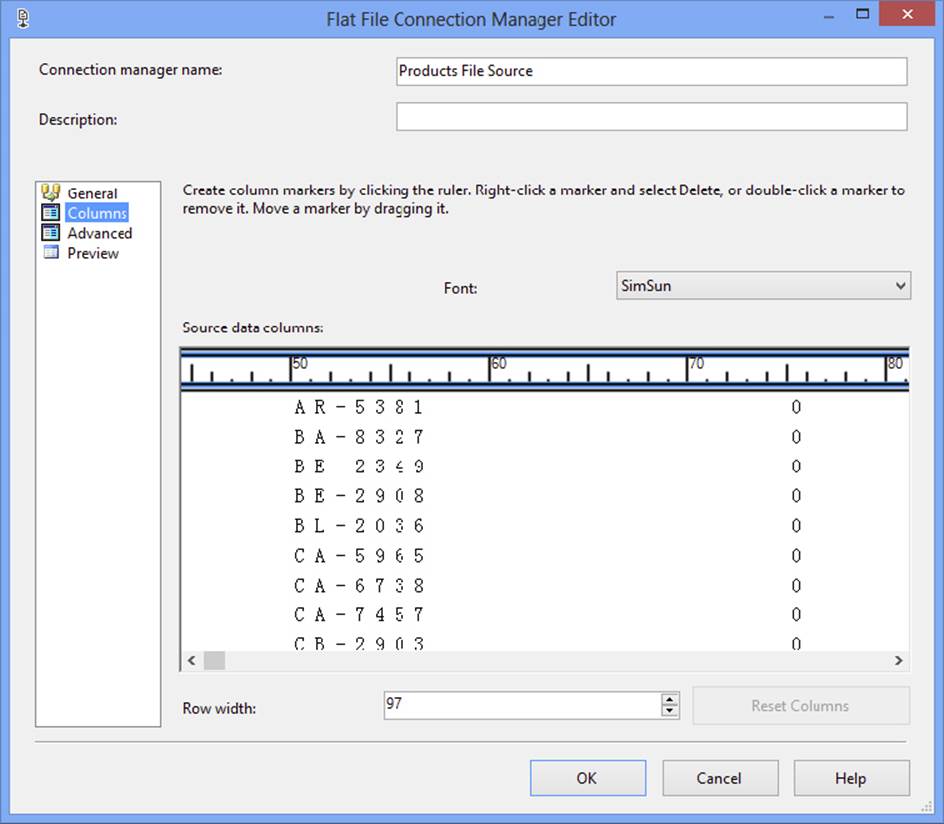

FIGURE 14-33

9. Now you need to identify the fixed-width columns by clicking in the text space right before each column starts. You need to do this for every column.

10.Click the Advanced property page tab and then click the Suggest Types button, which opens the Suggest Column Types window. Click OK to have SSIS scan the file and then suggest data types for the file.

11.While you are still in the Advanced Editor, you should see Column 0 through Column 2. Click Column 0, and in the properties in the right window, change the Name property to ProductName.

12.Click Column 2 and change its Name to ProductNumber.

13.For Column 2, change the Name property to ListPrice and change the DataType dropdown to [DT_CY], as Figure 14-34 shows.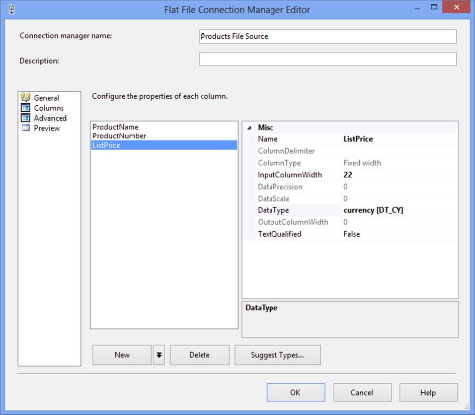

FIGURE 14-34

14.Select OK to save the Flat File Connection Manager properties.

15.While still in the Flat File Source Editor, select the Columns tab, and verify that all the columns are checked in the Available External Columns list.

16.Select OK to save the properties.

17.From the Data Flow Toolbox, drag a Multicast Transformation to the Data Flow workspace and connect the blue data path from the Flat File Source adapter to the Multicast.

At this point, you would usually create downstream transformations or a destination. For the purpose of this example, run the package and observe how the flat file data is extracted into the Data Flow. Nothing is done with it, but it demonstrates how to extract data from a flat file.

ODBC

ODBC stands for Open Database Connectivity and is a technology connection standard for passing data between systems that is widely used today for access to RDBMS systems that do not have an OLE DB or ADO.NET provider.

Just like the standard OLE DB providers, ODBC is part of the Windows operating system, included in the MDAC (Microsoft Data Access Components) when the operating system is installed. However, ODBC works differently than the OLE DB providers in that you need to set up the connection information through an applet in the Administrative Tools called Data Sources (ODBC). The OLE DB connections, conversely, are managed directly by the applications and not by the OS. There are some similarities in connecting to Oracle because for Oracle connections, you need to have the configuration managed external to SSIS as well.

For SSIS in SQL 2014, ODBC connectivity is handled by source and destination adapters in the Data Flow. Therefore, the process to get access to an ODBC Source or Destination is to first configure the connection in the Data Sources (ODBC) applet and then reference the ODBC connection through the ODBC adapters in SSIS.

The following example uses public domain data from a DBF Source file, which can be accessed through an ODBC connection. The file is a set of records containing a list of U.S. cities and their properties and is available for download with this book’s examples in a file called tl_2013_13_concity.dbf. Use the following steps to connect to an ODBC-based source:

1. The first step varies according to the machine on which you are working:

· For machines with an X64 version of Windows installed, go to a run command and enter the following to bring up the 32-bit version of the ODBC administrator program: %systemdrive%\Windows\SysWoW64\odbcad32.exe. Because you are developing a package in SSDT, which is a 32-bit program, you need to make an entry in the 32-bit version of the ODBC administrator tool.

· If you are on a 32-bit machine, go to the Administrative Tools folder found in the Control Panel list. Then open the Data Sources (ODBC) application from this list of administrative programs. Figure 14-35 shows the ODBC Data Source Administrator tool.

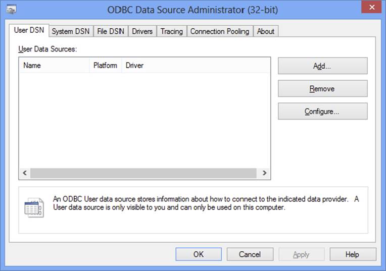
FIGURE 14-35

2. Switch to the System DSN tab, where you will create the ODBC reference (so it is accessible to all users) and click Add.

3. In the Create New Data Source window, scroll down and choose the Microsoft dBase Driver (not the Microsoft Access dBase Driver) and select Finish.

4. In the ODBC dBase Setup window, change the Data Source Name to US_Cities and uncheck the Use Current Directory checkbox.

5. Click the Select Directory button and navigate to the folder where the tl_2013_13_concity.dbf file is located (provided with the book’s online files). Select OK to save the directory path. Figure 14-36 shows the ODBC dBASE Setup dialog (in this case, the .dbf file is located at the root of the c:\ProSSIS\data drive).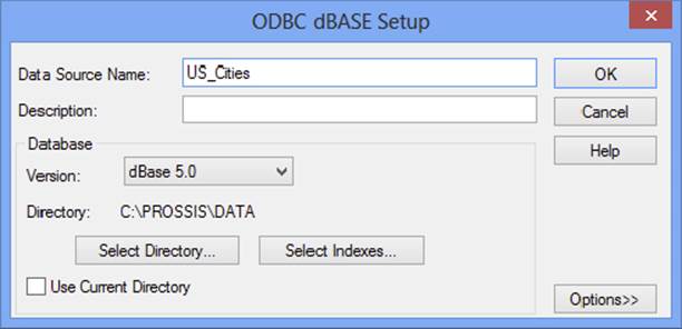

FIGURE 14-36

6. Select OK in the ODBC dBASE Setup dialog and OK in the ODBC Data Sources Administrator to save the US Cities DBF reference.

7. Create a new package in SSIS and a new Data Flow.

8. Drag an ODBC Source adapter from the Toolbox into the Data Flow workspace and double-click the ODBC Source to open its editor.

9. In the ODBC Source Editor, click the New button next to the ODBC Connection Manager window.

10.Select the New button again when the Configure ODBC Connection Manager dialog opens.

11.The Connection Manager dialog enables you to reference the DBF file through an ODBC connection. Select US_Cities from the list, as shown in Figure 14-37.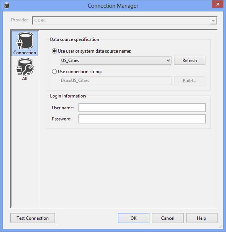

FIGURE 14-37

12.Select OK in the Connection Manager dialog, and OK in the Configure ODBC Connection Manager dialog, which will return you to the ODBC Source Editor with the US_Cities connection selected.

13.In the “Name of the table or the view” dropdown list, choose the tl_2013_13_concity table in the list. Figure 14-38 shows the ODBC Source Editor dialog.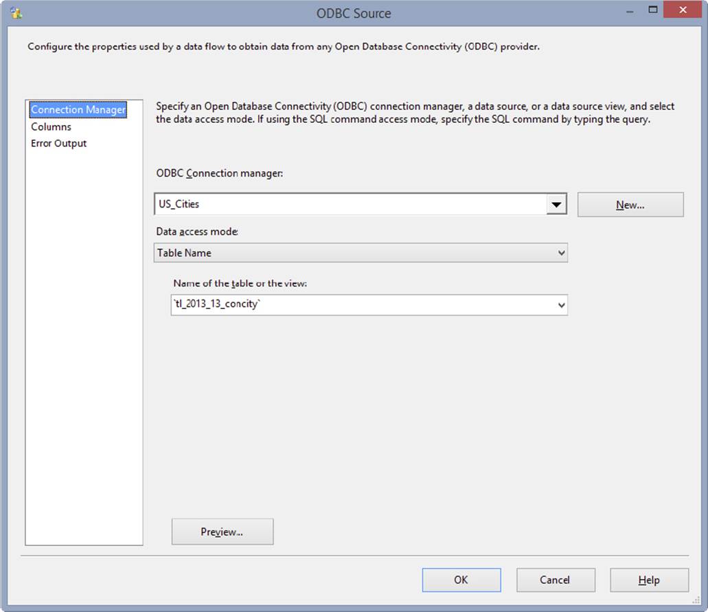

FIGURE 14-38

14.Click the Columns property page tab to bring up a list of the columns available in this file.

15.Select OK to save the changes of the ODBC Source adapter.

16.To demonstrate loading this ODBC Source to a destination table, drag an OLE DB Destination adapter and connect the blue data path from the ODBC Source adapter to the OLE DB Destination adapter.

17.Configure the OLE DB Destination to load the data to a new table in one of the sample databases.

After you run this new package, use SSMS to open the table you just loaded and observe the loaded results.

If you have a need to load data to an ODBC Destination, the process is very similar, but you use the ODBC Destination adapter to perform this operation.

OTHER HETEROGENEOUS SOURCES

Beyond the heterogeneous data already discussed, you may come across other non-SQL Server systems to which you need access. Examples of this include DB2 or Teradata or applications like SalesForce, SAP, or PeopleSoft or even decision support systems (DSS). A general approach in connecting to these is to first search for an OLE DB provider, so that you can then use the OLE DB adapters in the Data Flow to extract and load data to the system.

The Codeplex SSIS Community Tasks and Components list gives several of the available third-party connection managers (free and paid) that you can use with SSIS at http://ssisctc.codeplex.com/.

Also, if you need to connect to an IBM DB2 system, an OLE DB provider is available from Microsoft at http://msdn2.microsoft.com/en-us/library/Aa213281.aspx. This provider was originally used in the Host Integration Server but has been made available for broad use.

For SAP connectors, Microsoft has historically provided them with the SQL Server feature pack, which can be found on the Microsoft download site (www.microsoft.com/download). At the time of writing, the feature pack has not been released for SQL Server 2014, but these will be available when released.

If an OLE DB provider is not available from Microsoft, you can always check the company that owns the system to see if they provide a free OLE DB or ODBC driver. Be aware that sometimes it is not in their interest to make it easy to connect to their systems, so even if they do have a provider, it may be slow. Alternatively, some software companies sell providers. The following is a list of companies to research that can assist in expanding your connectivity options:

· Attunity (www.attunity.com) has several SSIS connectors including Teradata, BizTalk, and SharePoint. In SQL Server 2008, Microsoft licensed the use of the Oracle and Teradata Attunity connectors for SSIS and provided a free download from the Microsoft download site. As of this writing, the SSIS 2014 components have not yet been released, but check the Microsoft download site (www.microsoft.com/download) for latest updates.

· CozyRoc (www.cozyroc.com) has dozens of SSIS connectors, tasks, and transformations that you can use with SSIS, including connectors to Amazon S3 cloud, Microsoft Dynamics, and SharePoint to name a few.

· Data Direct (www.datadirect.com) sells data connection providers (ODBC and OLE DB) that can be installed on Windows operating systems. Some of the connections include Sybase, IBM DB2, Teradata, Informix, and Lotus Notes.

· Pragmatic Works (www.pragmaticworks.com) sells a product called Task Factory that is a collection of custom SSIS components including a destination for Oracle.

NOTE Some systems offer only APIs that enable you to connect to the data programmatically. In these cases, you can also use the Script Component as a source and leverage the system API. See Chapter 9 for more information about leveraging the Script Component.

SUMMARY

SSIS is capable of connecting to a variety of Data Sources for extraction and loading, but getting there may take a little bit of configuring. Data connects can sometimes be tricky, as they require the coordination of third-party software and SSIS adapters. The good news is that most sources are accessible in SSIS — whether through the standard built-in providers or through external providers that can be installed on your SSIS server.

So far this book has covered the basic techniques of building SSIS packages. You now have enough knowledge to put all the pieces together and build a more complex package. The next chapter focuses on how to guarantee that your SSIS packages will scale and work reliably.