Agile Data Science (2014)

Part I. Setup

Chapter 2. Data

This chapter introduces the dataset we will work on in the rest of the book: your own email inbox. It will also cover the kinds of tools we’ll be using, and our reasoning for doing so. Finally, it will outline multiple perspectives we’ll use in analyzing data for you to think about moving forward.

The book starts with data because in Agile Big Data, our process starts with the data.

NOTE

If you do not have a Gmail account, you will need to create one (at http://mail.google.com) and populate it with some email messages in order to complete the exercises in this chapter.

Email

Email is a fundamental part of the Internet. More than that, it is foundational, forming the basis for authentication for the Web and social networks. In addition to being abundant and well understood, email is complex, is rich in signal, and yields interesting information when mined.

We will be using your own email inbox as the dataset for the application we’ll develop in order to make the examples relevant. By downloading your Gmail inbox and then using it in the examples, we will immediately face a “big” or actually, a “medium” data problem—processing the data on your local machine is just barely feasible. Working with data too large to fit in RAM this way requires that we use scalable tools, which is helpful as a learning device. By using your own email inbox, we’ll enable insights into your own little world, helping you see which techniques are effective! This is cultivating data intuition, a major theme in Agile Big Data.

In this book, we use the same tools that you would use at petabyte scale, but in local mode on your own machine. This is more than an efficient way to process data; our choice of tools ensures that we only have to build it once, and it will scale up. This imparts simplicity on everything that we do and enables agility.

Working with Raw Data

Raw Email

Email’s format is rigorously defined in IETF RFC-5322 (Request For Comments by the Internet Engineering Taskforce). To view a raw email in Gmail, select a message and then select the “show original” option in the top-right drop-down menu (Figure 2-1).

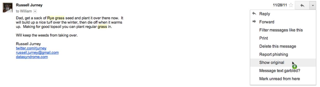
Figure 2-1. Gmail “show original” option

A raw email looks like this:

From: Russell Jurney <russell.jurney@gmail.com>

Mime-Version: 1.0 (1.0)

Date: Mon, 28 Nov 2011 14:57:38 -0800

Delivered-To: russell.jurney@gmail.com

Message-ID: <4484555894252760987@unknownmsgid>

Subject: Re: Lawn

To: William Jurney <******@hotmail.com>

Content-Type: text/plain; charset=ISO-8859-1

Dad, get a sack of Rye grass seed and plant it over there now. It

will build up a nice turf over the winter, then die off when it warms

up. Making for good topsoil you can plant regular grass in.

Will keep the weeds from taking over.

Russell Jurney datasyndrome.com

This is called semistructured data.

Structured Versus Semistructured Data

Wikipedia defines semistructured data as:

A form of structured data that does not conform with the formal structure of tables and data models associated with relational databases but nonetheless contains tags or other markers to separate semantic elements and enforce hierarchies of records and fields within the data.

This is in contrast to relational, structured data, which breaks data up into rigorously defined schemas before analytics begin for more efficient querying therafter. A structured view of email is demonstrated in the Berkeley Enron dataset by Andrew Fiore and Jeff Heer, shown in Figure 2-2.

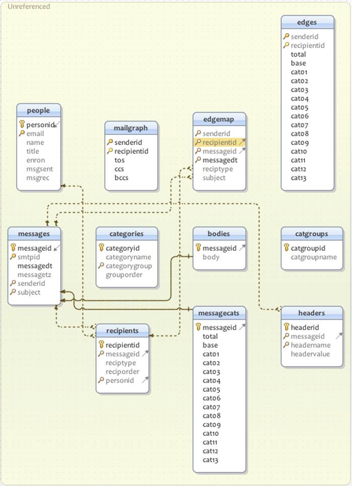
Figure 2-2. Enron email schema

SQL

To query a relational, structured schema, we typically use declarative programming languages like SQL. In SQL, we specify what we want, rather than what to do. This is different than declarative programming. In SQL, we specify the desired output rather than a set of operations on our data. A SQL query against the Enron relational email dataset to retrieve a single email in its entirety looks like this:

select m.smtpid as id,

m.messagedt as date,

s.email as sender,

(select GROUP_CONCAT(CONCAT(r.reciptype, ':', p.email) SEPARATOR ' ')

from recipients r

join people p

on r.personid=p.personid

where r.messageid = 511) as to_cc_bcc,

m.subject as subject,

SUBSTR(b.body, 1, 200) as body

from messages m

join people s

on m.senderid=s.personid

join bodies b

on m.messageid=b.messageid

where m.messageid=511;

| <25772535.1075839951307.JavaMail.evans@thyme> | 2002-02-02 12:56:33

| pete.davis@enron.com |

to:pete.davis@enron.com cc:albert.meyers@enron.com cc:bill.williams@enron.com

cc:craig.dean@enron.com

cc:geir.solberg@enron.com cc:john.anderson@enron.com cc:mark.guzman@enron.com

cc:michael.mier@enron.com

cc:pete.davis@enron.com cc:ryan.slinger@enron.com bcc:albert.meyers@enron.com

bcc:bill.williams@enron.com

bcc:craig.dean@enron.com bcc:geir.solberg@enron.com bcc:john.anderson@enron.com

bcc:mark.guzman@enron.com

bcc:michael.mier@enron.com bcc:pete.davis@enron.com bcc:ryan.slinger@enron.com

| Schedule Crawler:

HourAhead Failure | Start Date: 2/2/02; HourAhead hour: 11;

HourAhead schedule download failed. Manual intervention required. |

Note how complex this query is to retrieve a basic record. We join three tables and use a subquery, the special MySQL function GROUP_CONCAT as well as CONCAT and SUBSTR. Relational data almost discourages us from viewing data in its original form by requiring us to think in terms of the relational schema and not the data itself in its original, denormalized form. This complexity affects our entire analysis, putting us in “SQL land” instead of document reality.

Also note that defining the preceding tables is complex in and of itself:

CREATE TABLE bodies (

messageid int(10) unsigned NOT NULL default '0',

body text,

PRIMARY KEY (messageid)

) TYPE=MyISAM;

CREATE TABLE categories (

categoryid int(10) unsigned NOT NULL auto_increment,

categoryname varchar(255) default NULL,

categorygroup int(10) unsigned default NULL,

grouporder int(10) unsigned default NULL,

PRIMARY KEY (categoryid),

KEY categories_categorygroup (categorygroup)

) TYPE=MyISAM;

CREATE TABLE catgroups (

catgroupid int(10) unsigned NOT NULL default '0',

catgroupname varchar(255) default NULL,

PRIMARY KEY (catgroupid)

) TYPE=MyISAM;

CREATE TABLE edgemap (

senderid int(10) unsigned default NULL,

recipientid int(10) unsigned default NULL,

messageid int(10) unsigned default NULL,

messagedt timestamp(14) NOT NULL,

reciptype enum('bcc','cc','to') default NULL,

subject varchar(255) default NULL,

KEY senderid (senderid,recipientid),

KEY messageid (messageid),

KEY messagedt (messagedt),

KEY senderid_2 (senderid),

KEY recipientid (recipientid)

) TYPE=MyISAM;

CREATE TABLE edges (

senderid int(10) unsigned default NULL,

recipientid int(10) unsigned default NULL,

total int(10) unsigned NOT NULL default '0',

base int(10) unsigned NOT NULL default '0',

cat01 int(10) unsigned NOT NULL default '0',

cat02 int(10) unsigned NOT NULL default '0',

cat03 int(10) unsigned NOT NULL default '0',

cat04 int(10) unsigned NOT NULL default '0',

cat05 int(10) unsigned NOT NULL default '0',

cat06 int(10) unsigned NOT NULL default '0',

cat07 int(10) unsigned NOT NULL default '0',

cat08 int(10) unsigned NOT NULL default '0',

cat09 int(10) unsigned NOT NULL default '0',

cat10 int(10) unsigned NOT NULL default '0',

cat11 int(10) unsigned NOT NULL default '0',

cat12 int(10) unsigned NOT NULL default '0',

cat13 int(10) unsigned NOT NULL default '0',

UNIQUE KEY senderid (senderid,recipientid)

) TYPE=MyISAM;

CREATE TABLE headers (

headerid int(10) unsigned NOT NULL auto_increment,

messageid int(10) unsigned default NULL,

headername varchar(255) default NULL,

headervalue text,

PRIMARY KEY (headerid),

KEY headers_headername (headername),

KEY headers_messageid (messageid)

) TYPE=MyISAM;

CREATE TABLE messages (

messageid int(10) unsigned NOT NULL auto_increment,

smtpid varchar(255) default NULL,

messagedt timestamp(14) NOT NULL,

messagetz varchar(20) default NULL,

senderid int(10) unsigned default NULL,

subject varchar(255) default NULL,

PRIMARY KEY (messageid),

UNIQUE KEY smtpid (smtpid),

KEY messages_senderid (senderid),

KEY messages_subject (subject)

) TYPE=MyISAM;

CREATE TABLE people (

personid int(10) unsigned NOT NULL auto_increment,

email varchar(255) default NULL,

name varchar(255) default NULL,

title varchar(255) default NULL,

enron tinyint(3) unsigned default NULL,

msgsent int(10) unsigned default NULL,

msgrec int(10) unsigned default NULL,

PRIMARY KEY (personid),

UNIQUE KEY email (email)

) TYPE=MyISAM;

--

--

CREATE TABLE recipients (

recipientid int(10) unsigned NOT NULL auto_increment,

messageid int(10) unsigned default NULL,

reciptype enum('bcc','cc','to') default NULL,

reciporder int(10) unsigned default NULL,

personid int(10) unsigned default NULL,

PRIMARY KEY (recipientid),

KEY messageid (messageid)

) TYPE=MyISAM;

By contrast, in Agile Big Data we use dataflow languages to define the form of our data in code, and then we publish it directly to a document store without ever formally specifying a schema! This is optimized for our process: doing data science, where we’re deriving new information from existing data. There is no benefit to externally specifying schemas in this context—it is pure overhead. After all, we don’t know what we’ll wind up with until it’s ready! Data science will always surprise.

However, relational structure does have benefits. We can see what time users send emails very easily with a simple select/group by/order query:

select senderid as id,

hour(messagedt) as sent_hour,

count(*)

from messages

where senderid=511

group by

senderid,

m_hour

order by

senderid,

m_hour;

which results in this simple table:

+----------+--------+----------+

| senderid | m_hour | count(*) |

+----------+--------+----------+

| 1 | 0 | 4 |

| 1 | 1 | 3 |

| 1 | 3 | 2 |

| 1 | 5 | 1 |

| 1 | 8 | 3 |

| 1 | 9 | 1 |

| 1 | 10 | 5 |

| 1 | 11 | 2 |

| 1 | 12 | 2 |

| 1 | 14 | 1 |

| 1 | 15 | 5 |

| 1 | 16 | 4 |

| 1 | 17 | 1 |

| 1 | 19 | 1 |

| 1 | 20 | 1 |

| 1 | 21 | 1 |

| 1 | 22 | 1 |

| 1 | 23 | 1 |

+----------+--------+----------+

Relational databases split data up into tables according to its structure and precompute indexes for operating between these tables. Indexes enable these systems to be responsive on a single computer. Declarative programming is used to query this structure.

This kind of declarative programming is ideally suited to consuming and querying structured data in aggregate to produce simple charts and figures. When we know what we want, we can efficiently tell the SQL engine what that is, and it will compute the relations for us. We don’t have to worry about the details of the query’s execution.

NoSQL

In contrast to SQL, when building analytics applications we often don’t know the query we want to run. Much experimentation and iteration is required to arrive at the solution to any given problem. Data is often unavailable in a relational format. Data in the wild is not normalized; it is fuzzy and dirty. Extracting structure is a lengthy process that we perform iteratively as we process data for different features.

For these reasons, in Agile Big Data we primarily employ imperative languages against distributed systems. Imperative languages like Pig Latin describe steps to manipulate data in pipelines. Rather than precompute indexes against structure we don’t yet have, we use many processing cores in parallel to read individual records. Hadoop and work queues make this possible.

In addition to mapping well to technologies like Hadoop, which enables us to easily scale our processing, imperative languages put the focus of our tools where most of the work in building analytics applications is: in one or two hard-won, key steps where we do clever things that deliver most of the value of our application.

Compared to writing SQL queries, arriving at these clever operations is a lengthy and often exhaustive process, as we employ techniques from statistics, machine learning, and social network analysis. Thus, imperative programming fits the task.

To summarize, when schemas are rigorous, and SQL is our lone tool, our perspective comes to be dominated by tools optimized for consumption, rather than mining data. Rigorously defined schemas get in the way. Our ability to connect intuitively with the data is inhibited. Working with semistructured data, on the other hand, enables us to focus on the data directly, manipulating it iteratively to extract value and to transform it to a product form. In Agile Big Data, we embrace NoSQL for what it enables us to do.

Serialization

Although we can work with semistructured data as pure text, it is still helpful to impose some kind of structure to the raw records using a schema. Serialization systems give us this functionality. Available serialization systems include the following:

Although it is the least mature of these options, we’ll choose Avro. Avro allows complex data structures, it includes a schema with each file, and it has support in Apache Pig. Installing Avro is easy, and it requires no external service to run.

We’ll define a single, simple Avro schema for an email document as defined in RFC-5322. It is well and good to define a schema up front, but in practice, much processing will be required to extract all the entities in that schema. So our initial schema might look very simple, like this:

{

"type":"record",

"name":"RawEmail",

"fields":

[

{

"name":"thread_id",

"type":["string", "null"],

"doc":""

},

{

"name":"raw_email",

"type": ["string", "null"]

}

]

}

We might extract only a thread_id as a unique identifier, and then store the entire raw email string in a field on its own. If a unique identifier is not easy to extract from raw records, we can generate a UUID (universally unique identifier) and add it as a field.

Our job as we process data, then, is to add fields to our schema as we extract them, all the while retaining the raw data in its own field if we can. We can always go back to the mother source.

Extracting and Exposing Features in Evolving Schemas

As Pete Warden notes in his talk “Embracing the Chaos of Data”, most freely available data is crude and unstructured. It is the availability of huge volumes of such ugly data, and not carefully cleaned and normalized tables, that makes it “big data.” Therein lies the opportunity in mining crude data into refined information, and using that information to drive new kinds of actions.

Extracted features from unstructured data get cleaned only in the harsh light of day, as users consume them and complain; if you can’t ship your features as you extract them, you’re in a state of free fall. The hardest part of building data products is pegging entity and feature extraction to products smaller than your ultimate vision. This is why schemas must start as blobs of unstructured text and evolve into structured data only as features are extracted.

Features must be exposed in some product form as they are created, or they will never achieve a product-ready state. Derived data that lives in the basement of your product is unlikely to shape up. It is better to create entity pages to bring entities up to a “consumer-grade” form, to incrementally improve these entities, and to progressively combine them than to try to expose myriad derived data in a grand vision from the get-go.

While mining data into well-structured information, using that information to expose new facts and make predictions that enable actions offers enormous potential for value creation. Data is brutal and unforgiving, and failing to mind its true nature will dash the dreams of the most ambitious product manager.

As we’ll see throughout the book, schemas evolve and improve, and so do features that expose them. When they evolve concurrently, we are truly agile.

Data Pipelines

We’ll be working with semistructured data in data pipelines to extract and display its different features. The advantage of working with data in this way is that we don’t invest time in extracting structure unless it is of interest and use to us. Thus, in the principles of KISS (Keep It Simple, Stupid!) and YAGNI (You Ain’t Gonna Need It), we defer this overhead until the time of need. Our toolset helps make this more efficient, as we’ll see in Chapter 3.

Figure 2-3 shows a data pipeline to calculate the number of emails sent between two email addresses.

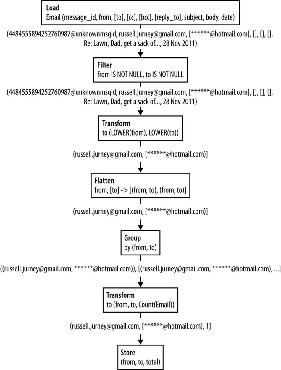
Figure 2-3. Simple dataflow to count the number of emails sent between two email addresses

While this dataflow may look complex now if you’re used to SQL, you’ll quickly get used to working this way and such a simple flow will become second nature.

Data Perspectives

To start, it is helpful to highlight different ways of looking at email. In Agile Big Data, we employ varied perspectives to inspect and mine data in multiple ways because it is easy to get stuck thinking about data in one or two ways that you find productive. Next, we’ll discuss the different perspectives on email data we’ll be using throughout the book.

Networks

A social network is a group of persons (egos) and the connections or links between them. These connections may be directed, as in “Bob knows Sara.” Or they may be undirected: “Bob and Sara are friends.” Connections may also have a connection strength, or weight. “Bob knows Sara well,” (on a scale of 0 to 1) or “Bob and Sara are married” (on a scale of 0 to 1).

The sender and recipients of an email via the from, to, cc, and bcc fields can be used to create a social network. For instance, this email defines two entities, russell.jurney@gmail.com and ******@hotmail.com.

From: Russell Jurney <russell.jurney@gmail.com>

To: ******* Jurney <******@hotmail.com>

The message itself implies a link between them. We can represent this as a simple social network, as shown in Figure 2-4.

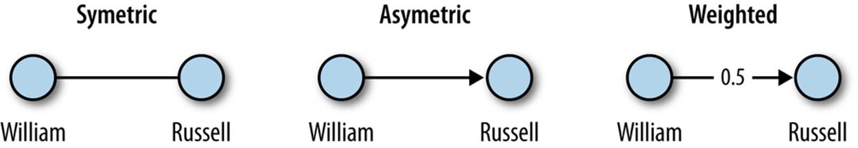
Figure 2-4. Social network dyad

Figure 2-5 depicts a more complex social network.

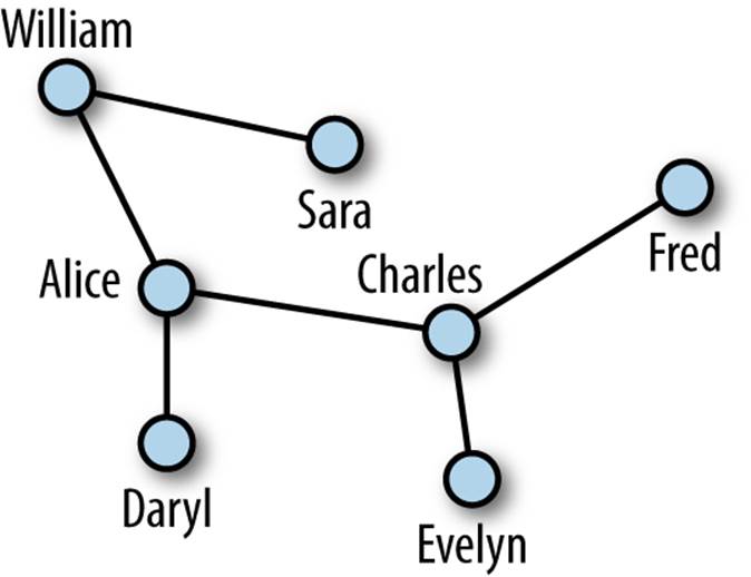
Figure 2-5. Social network

Figure 2-6 shows a social network of some 200 megabytes of emails from Enron.

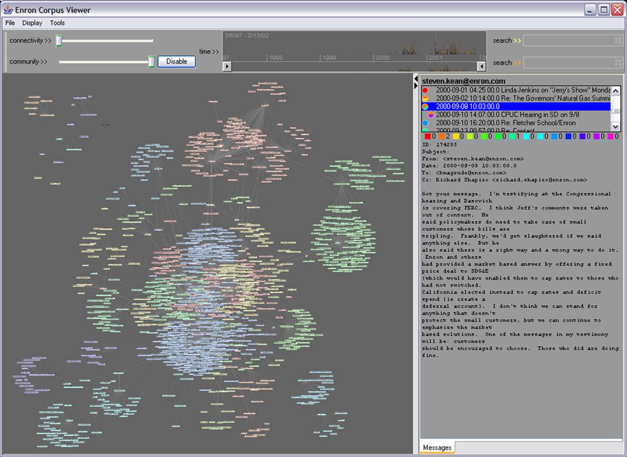
Figure 2-6. Enron corpus viewer, by Jeffrey Heer and Andrew Fiore

Social network analysis, or SNA, is the scientific study and analysis of social networks. By modeling our inbox as a social network, we can draw on the methods of SNA (like PageRank) to reach a deeper understanding of the data and of our interpersonal network. Figure 2-7 shows such an analysis applied to the Enron network.

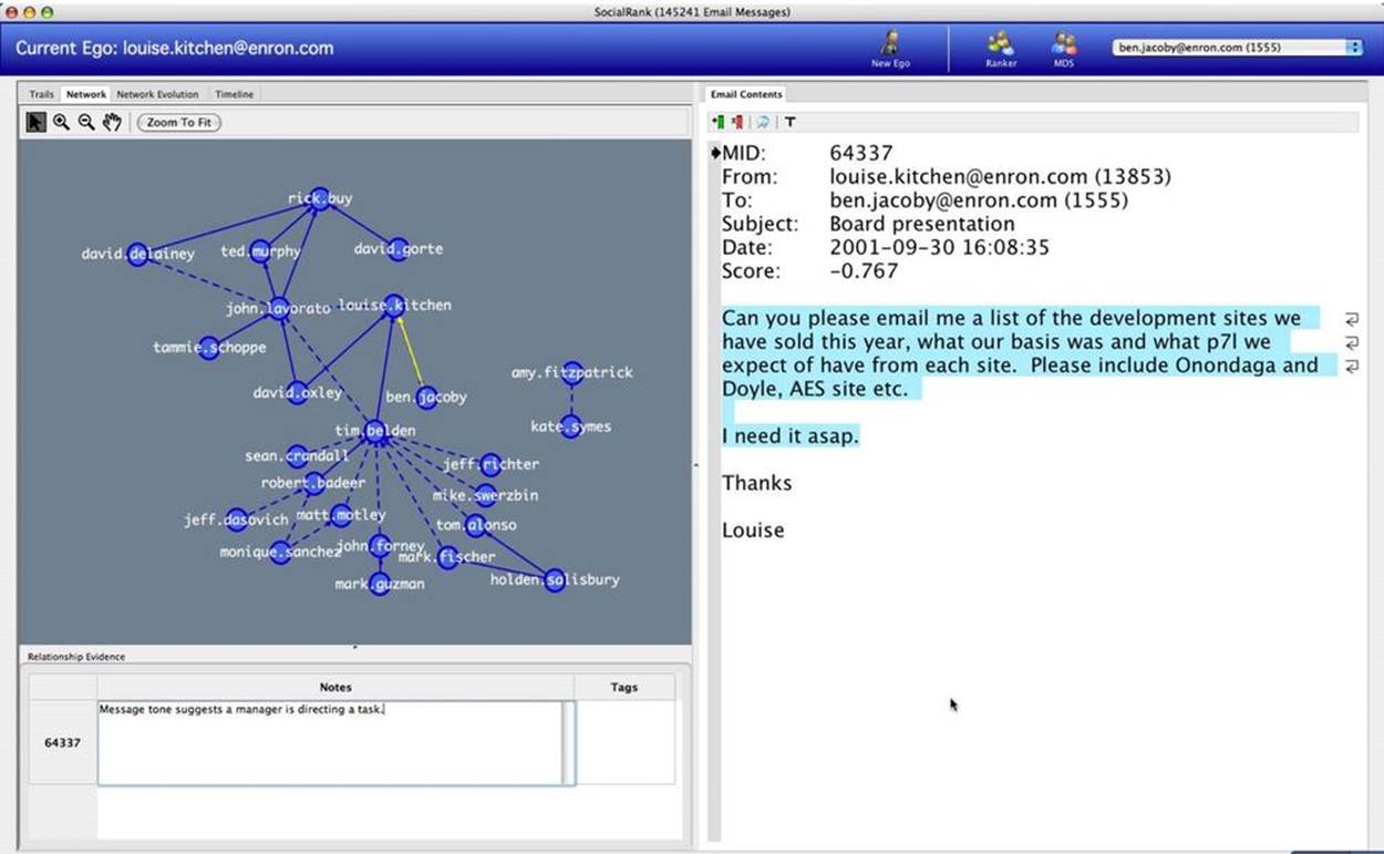
Figure 2-7. Enron SocialRank, by Jaime Montemayor, Chris Diehl, Mike Pekala, and David Patrone

Time Series

A time series is a sequence of data points ordered by a timestamp recorded with each value. Time series allow us to see changes and trends in data over time. All emails have timestamps, so we can represent a series of emails as a time series, as Figure 2-8 demonstrates.

Date: Mon, 28 Nov 2011 14:57:38 -0800

Looking at several other emails, we can plot the raw data in a time series.

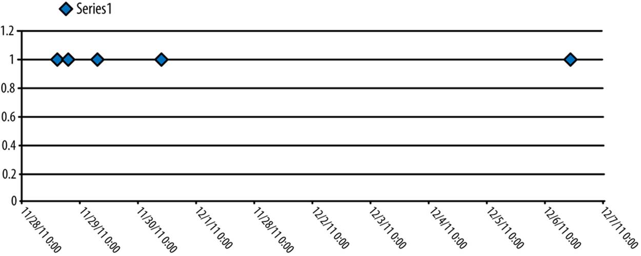
Figure 2-8. Raw time series

Since we aren’t looking at another value associated with the time series, we can see the data more clearly by bucketing it by day (see Figure 2-9). This will tell us how many emails were sent between these two addresses per day.

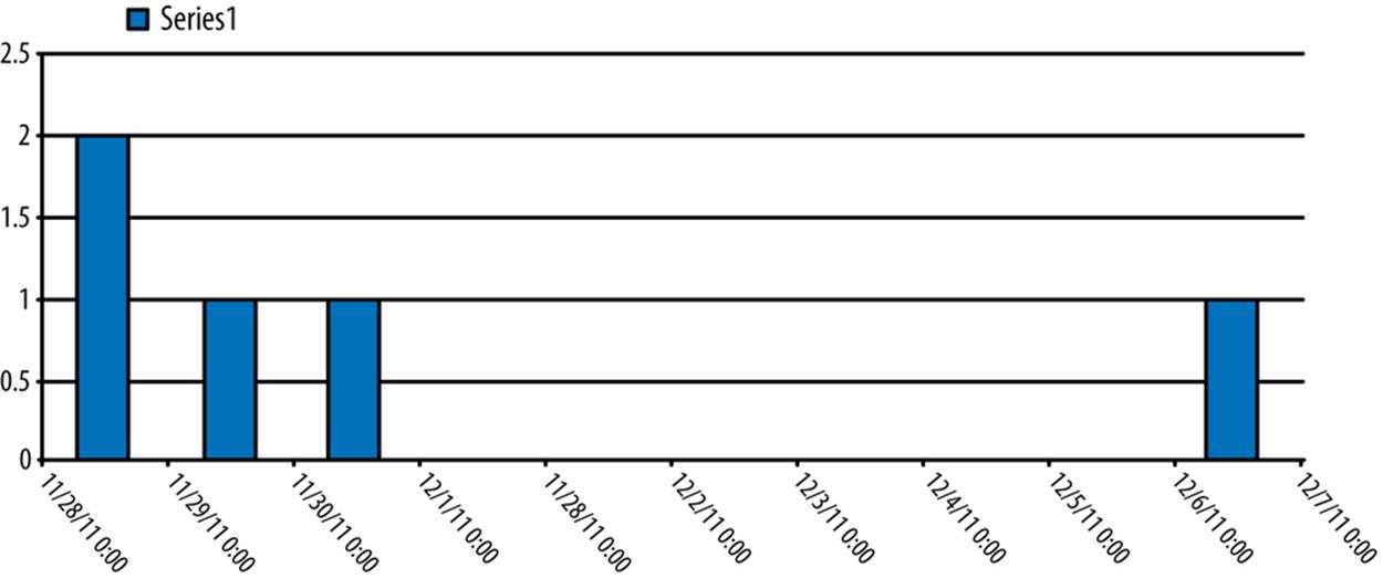
Figure 2-9. Grouped time series

Time series analysis might tell us when we most often receive email from a particular person or even what that person’s work schedule is.

Natural Language

The meat of an email is its text content. Despite the addition of MIME for multimedia attachments, email is still primarily text.

Subject: Re: Lawn

Content-Type: text/plain; charset=ISO-8859-1

Dad, get a sack of Rye grass seed and plant it over there now. It

will build up a nice turf over the winter, then die off when it warms

up. Making for good topsoil you can plant regular grass in.

Will keep the weeds from taking over.

Russell Jurney

twitter.com/rjurney

russell.jurney@gmail.com

datasyndrome.com

We might analyze the body of the email by counting its word frequency. Once we remove noncoding common stopwords (like of and it), this looks like Figure 2-10.

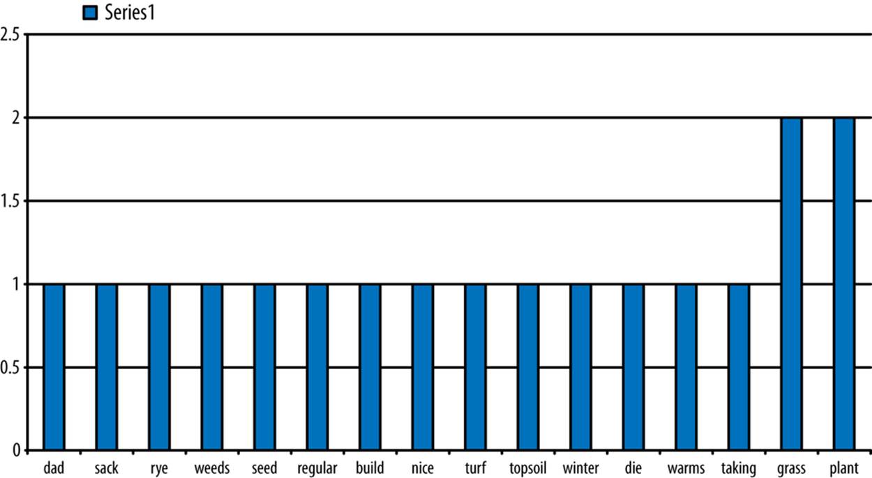
Figure 2-10. Email body word frequency

We might use this word frequency to infer that the topics of the email are plant and grass, as these are the most common words. Processing natural language in this way helps us to extract properties from semistructured data to make it more structured. This enables us to incorporate these structured properties into our analysis.

A fun way to show word frequency is via a wordle, illustrated in Figure 2-11.

Figure 2-11. Email body wordle

Probability

In probability theory, we model seemingly random processes by counting the occurrence and co-occurence of different properties in our data to create probability distributions. We can then employ these probability distributions to make suggestions and to classify entities into different categories.

We can use probability distributions to make predictions. For instance, we might create a probability distribution for our sent emails using the from, to, and cc fields. Given that our email address, russell.jurney@gmail.com, appears in the from field, and another email address appears in the tofield, what is the chance that another email will appear cc‘d?

In this case, our raw data is the to, from, and cc fields from each email:

From: Russell Jurney <russell.jurney@gmail.com>

To: ****** Jurney <******@hotmail.com>

Cc: Ruth Jurney <****@hotmail.com>

First, we count the pairs of from email addresses with to email addresses. This is called the co-occurrence of these two properties. Let’s highlight one pair in particular, those emails between O’Reilly editor Mike Loukides and me (Table 2-1).

Table 2-1. Totals for to, from pairs

Dividing these values by the total number of emails gives us a probability distribution characterizing the odds that any given email from our email address will be to any given email (Table 2-2).

Table 2-2. P(to|from): probability of to, given from

Finally, we list the probabilities for a pair recipients co-occurring, given that the first address appears in an email (Table 2-3).

Table 2-3. P(cc|from ∩ to): probability of cc, given from and to

We can then use this data to show who else is likely to appear in an email, given a single address. This data can be used to drive features like Gmail’s suggested recipients feature, as shown in Figure 2-12.

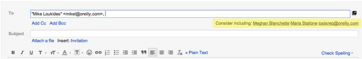
Figure 2-12. Gmail suggested recipients

We’ll see later how we can use Bayesian inference to make reasonable suggestions for recipients, even when Table 2-3 is incomplete.

Conclusion

As we’ve seen, viewing semistructured data according to different algorithms, structures, and perspectives informs feature development more than normalizing and viewing it in structured tables does. We’ll be using the perspectives defined in this chapter to create features throughout the book, as we climb the data-value pyramid. In the next chapter, you’ll learn how to specify schemas in our analytic stores using Apache Pig directly.