Agile Data Science (2014)

Part II. Climbing the Pyramid

Chapter 6. Visualizing Data with Charts

In the next step, our second agile sprint, we will start building charts from our data (Figure 6-1).

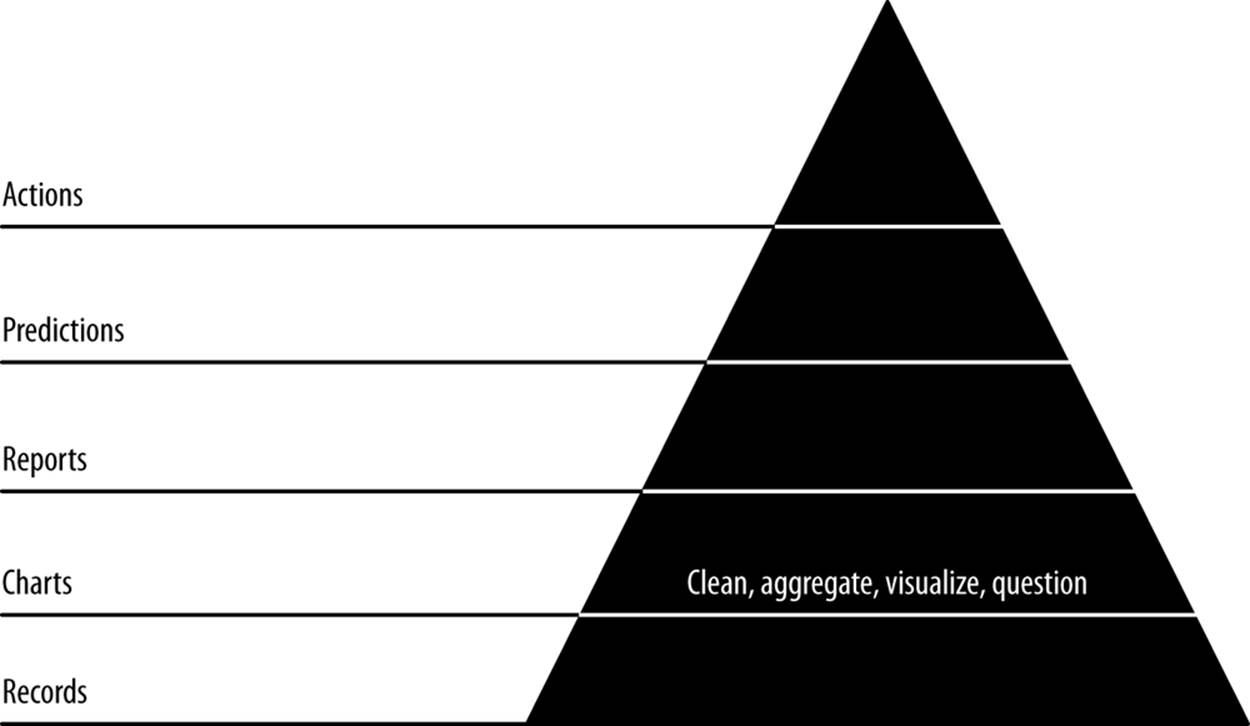
Figure 6-1. Level 2: visualizing with charts

Charts are our first view into our data in aggregate, mapping the properties of many records into visual representations that help us understand and navigate further and expose entities and concepts in our data. Our goals in this step are to publish charts to generate interest in our data and get users interacting with it, to build reusable tools that will help us explore our data interactively in reports in the next step, and to begin extracting structure and entities from our data so that we can create new features and insights with this structure.

Code examples for this chapter are available at https://github.com/rjurney/Agile_Data_Code/tree/master/ch06. Clone the repository and follow along!

git clone https://github.com/rjurney/Agile_Data_Code.git

Good Charts

A good chart is anything users find interesting enough to visualize and that users respond to. Expect to throw many charts away until you find good ones—don’t try to specify them up front or you will be disappointed. Instead, try to use your intuition and curiosity to add charts organically.

You can create charts in an ad hoc way at first, but as you progress, your workflow should become increasingly automated and reproducible.

Well-formed URLs with slugs generalize, so one chart works for anything. Good charts are those that get clicked, so get users involved. Later, we’ll improve and extend successful charts into interactive reports.

Extracting Entities: Email Addresses

An email address is an ego acting through a certain address or context (this is a simplification, because one person may have multiple email addresses, but an email address is a reasonable approximation of an ego). In this chapter, we will create a new entity for each email address in our inbox and then create interesting data to chart, display, and interact with.

Extracting Emails

We start by creating an index of all emails in which any given email address appears in the from/to/cc/bcc fields. This is a pattern: when you’re creating a new entity, always first link it to the atomic base records. Note that we can achieve this mapping in two ways.

The first option is using Pig to group emails by email addresses. This method puts all of our processing at the far backend in batch, which could be desirable for very large data. The second method is to use ElasticSearch Facets to query our email index just as we have before, but with different handling in our web application.

We group our emails in Pig and store them in MongoDB. We do this because we intend to use this data in other features via JOINs, and while Wonderdog enables reading data from ElasticSearch, it is important to have a copy of this data on reliable bulk storage, where it is truly persistent. We know we can easily and arbitrarily scale operations on Hadoop.

We’ll need to project each to/from/cc/bcc address with the message ID of that email, merge these header/address parts together by email, and then group by address to get a list of message IDs per address, and a list of addresses per message ID. Check out ch06/emails_per_address.pig, as shown in Example 6-1.

Example 6-1. Messages per email address

/* Avro uses json-simple, and is in piggybank until Pig 0.12, where AvroStorage and

TrevniStorage are builtins */

DEFINE AvroStorage org.apache.pig.piggybank.storage.avro.AvroStorage();

/* MongoDB libraries and configuration */

DEFINE MongoStorage com.mongodb.hadoop.pig.MongoStorage();

set default_parallel 10

set mapred.map.tasks.speculative.execution false

set mapred.reduce.tasks.speculative.execution false

/* Macro to filter emails according to existence of header pairs:

[from, to, cc, bcc, reply_to]

Then project the header part, message_id, and subject, and emit them, lowercased.

Note: you can't paste macros into Grunt as of Pig 0.11. You will have to execute

this file. */

DEFINE headers_messages(email, col) RETURNS set {

filtered = FILTER $email BY ($col IS NOT NULL);

flat = FOREACH filtered GENERATE

FLATTEN($col.address) AS $col, message_id, subject, date;

lowered = FOREACH flat GENERATE LOWER($col) AS address, message_id,

subject, date;

$set = FILTER lowered BY (address IS NOT NULL) and (address != '') and

(date IS NOT NULL);

}

/* Nuke the Mongo stores, as we are about to replace it. */

-- sh mongo agile_data --quiet --eval 'db.emails_per_address.drop(); exit();'

-- sh mongo agile_data --quiet --eval 'db.addresses_per_email.drop(); exit();'

rmf /tmp/emails_per_address.json

emails = load '/me/Data/test_mbox' using AvroStorage();

froms = foreach emails generate LOWER(from.address) as address, message_id, subject,

date;

froms = filter froms by (address IS NOT NULL) and (address != '') and

(date IS NOT NULL);

tos = headers_messages(emails, 'tos');

ccs = headers_messages(emails, 'ccs');

bccs = headers_messages(emails, 'bccs');

reply_tos = headers_messages(emails, 'reply_tos');

address_messages = UNION froms, tos, ccs, bccs, reply_tos;

/* Messages per email address, sorted by date desc. Limit to 50 to ensure rapid

access. */

emails_per_address = foreach (group address_messages by address) {

address_messages = order address_messages by date desc;

top_50 = limit address_messages 50;

generate group as address,

top_50.(message_id, subject, date) as emails;

}

store emails_per_address into 'mongodb://localhost/agile_data.emails_per_address'

using MongoStorage();

/* Email addresses per email */

addresses_per_email = foreach (group address_messages by message_id) generate group

as message_id, address_messages.(address) as addresses;

store addresses_per_email into 'mongodb://localhost/agile_data.addresses_per_email'

using MongoStorage();

Now we’ll check on our data in MongoDB. Check out ch06/mongo.js.

$ mongo agile_data

MongoDB shell version: 2.0.2

connecting to: agile_data

> show collections

addresses_per_id

ids_per_address

...

> db.emails_per_address.findOne()

{

"_id" : ObjectId("4ff7a38a0364f2e2dd6a43bc"),

"group" : "bob@clownshoes.org",

"email_address_messages" : [

{

"email_address" : "bob@clownshoes.org",

"message_id" : "B526D4C4-AA05-4A61-A0C5-9CF77373995C@123.org"

{

"email_address" : "bob@clownshoes.org",

"message_id" : "E58C12BA-0985-448B-BCD7-6C6C364FCF15@123.org"

{

"email_address" : "bob@clownshoes.org",

"message_id" : "593B0552-D007-453D-A3A8-B10288638E50@123.org"

{

"email_address" : "bob@clownshoes.org",

"message_id" : "3A211C33-FE82-4B2C-BE2F-16D5F7EB3A9C@123.org"

}

]

}

> db.addresses_per_email.findOne()

{

"_id" : ObjectId("50f71a5530047b9226f0dcb3"),

"message_id" : "4484555894252760987@unknownmsgid",

"addresses" : [

{

"address" : "russell.jurney@gmail.com"

{

"address" : "*******@hotmail.com"

}

]

}

> db.addresses_per_email.find({'email_address_messages': {$size: 4}})[0]

{

"_id" : ObjectId("4ff7ad800364f868d343e557"),

"message_id" : "4F586853.40903@touk.pl",

"email_address_messages" : [

{

"email_address" : "user@pig.apache.org",

"message_id" : "4F586853.40903@touk.pl"

{

"email_address" : "bob@plantsitting.org",

"message_id" : "4F586853.40903@touk.pl"

{

"email_address" : "billgraham@gmail.com",

"message_id" : "4F586853.40903@touk.pl"

{

"email_address" : "dvryaboy@gmail.com",

"message_id" : "4F586853.40903@touk.pl"

}

]

}

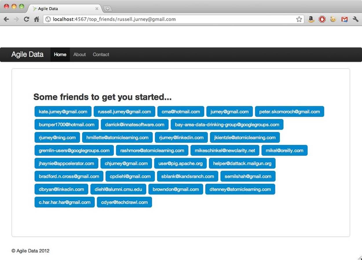
We can see how to query email addresses per message and messages per email address. This kind of data is foundational—it lets us add features to a page by directly rendering precomputed data. We’ll start by displaying these email addresses as a word cloud as part of the /email controller:

# Controller: Fetch an email and display it

@app.route("/email/<message_id>")

def email(message_id):

email = emails.find_one({'message_id': message_id})

addresses = addresses_per_email.find_one({'message_id': message_id})

return render_template('partials/email.html', email=email,

addresses=addresses['addresses'],

chart_json=json.dumps(sent_dist_records['sent_distribution']))

Our template is simple. It extends our application layout and relies on Bootstrap for styling.

{% if addresses -%}

<h3 style="margin-bottom: 5px;">Email Addresses</h2>

{% for item in addresses -%}

<a style="margin: 3px;" href="/address/{{ item['address'] }}

">{{ item['address'] }}</a>

</li>

{% endfor -%}

</ul>

{% endif -%}

And the result is simple:

Table of count of emails sent by hour for one email address

Visualizing Time

Let’s continue by computing a distribution of the times each email address sends emails. Check out ch06/sent_distributions.pig.

/* Set Home Directory - where we install software */

%default HOME `echo \$HOME/Software/`

/* Avro uses json-simple, and is in piggybank until Pig 0.12, where AvroStorage

and TrevniStorage are builtins */

DEFINE AvroStorage org.apache.pig.piggybank.storage.avro.AvroStorage();

DEFINE substr org.apache.pig.piggybank.evaluation.string.SUBSTRING();

DEFINE tohour org.apache.pig.piggybank.evaluation.datetime.truncate.ISOToHour();

/* MongoDB libraries and configuration */

DEFINE MongoStorage com.mongodb.hadoop.pig.MongoStorage();

set default_parallel 5

set mapred.map.tasks.speculative.execution false

set mapred.reduce.tasks.speculative.execution false

/* Macro to extract the hour portion of an iso8601 datetime string */

define extract_time(relation, field_in, field_out) RETURNS times {

$times = foreach $relation generate flatten($field_in.(address)) as $field_out,

substr(tohour(date), 11, 13) as sent_hour;

};

rmf /tmp/sent_distributions.avro

emails = load '/me/Data/test_mbox' using AvroStorage();

filtered = filter emails BY (from is not null) and (date is not null);

/* Some emails that users send to have no from entries, list email lists. These

addresses have reply_to's associated with them. Here we split reply_to

processing off to ensure reply_to addresses get credit for sending emails. */

split filtered into has_reply_to if (reply_tos is not null), froms if (reply_tos

is null);

/* For emails with a reply_to, count both the from and the reply_to as a sender. */

reply_to = extract_time(has_reply_to, reply_tos, from);

reply_to_froms = extract_time(has_reply_to, from, from);

froms = extract_time(froms, from, from);

all_froms = union reply_to, reply_to_froms, froms;

pairs = foreach all_froms generate LOWER(from) as sender_email_address,

sent_hour;

sent_times = foreach (group pairs by (sender_email_address, sent_hour)) generate

flatten(group) as (sender_email_address, sent_hour),

COUNT_STAR(pairs) as total;

/* Note the use of a sort inside a foreach block */

sent_distributions = foreach (group sent_times by sender_email_address) {

solid = filter sent_times by (sent_hour is not null) and (total is not null);

sorted = order solid by sent_hour;

generate group as address, sorted.(sent_hour, total) as sent_distribution;

};

store sent_distributions into '/tmp/sent_distributions.avro' using AvroStorage();

store sent_distributions into 'mongodb://localhost/agile_data.sent_distributions'

using MongoStorage();

NOTE

Datetimes in Pig are in ISO8601 format for a reason: that format is text sortable and manipulatable via truncation. In this case, we are truncating to the hour and then reading the hour figure.

substr(tohour(date), 11, 13) as sent_hour

Now, plumb the data to a browser with Flask:

# Display sent distributions for a give email address

@app.route('/sent_distribution/<string:sender>')

def sent_distribution(sender):

sent_dist_records = sent_distributions.find_one({'address': sender})

return render_template('partials/sent_distribution.html',

sent_distribution=sent_dist_records)

We start with a simple table in our Jinja2 HTML template, helped along by Bootstrap. Check out ch06/web/templates/partials/email.html.

{% if sent_distribution -%}

<thead>

<th>Total Sent</th>

</thead>

<tbody>

{% for item in sent_distribution['sent_distribution'] %}

<td style="white-space:nowrap;">{{ item['total'] }}</td>

</tr>

{% endfor %}

</tbody>

</table>

</div>

</div>

{% endif -%}

We can already tell our author is a night owl, but the shape of the distribution isn’t very clear in Figure 6-2.

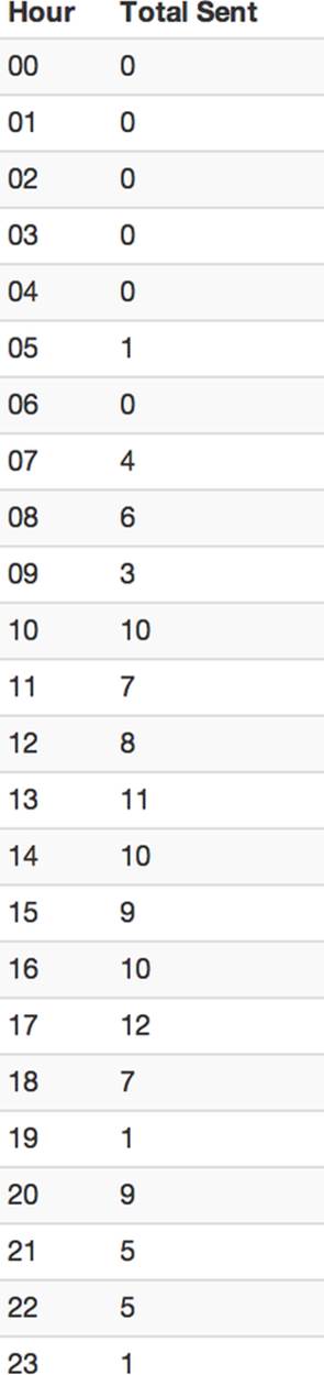
Table of count of emails sent by hour for one email address

Figure 6-2. Emails sent by hour table

To get a better view of the visualization, we create a simple bar chart using d3.js and nvd3.js, based on this example: http://mbostock.github.com/d3/tutorial/bar-1.html.

Now we update our web app to produce JSON for d3.

# Display sent distributions for a give email address

@app.route('/sent_distribution/<string:sender>')

def sent_distribution(sender):

sent_dist_records = sent_distributions.find_one({'address': sender})

return render_template('partials/sent_distribution.html',

chart_json=json.dumps(sent_dist_records['sent_distribution']),

sent_distribution=sent_dist_records)

And create the chart using nvd3:

{% if sent_distribution -%}

<h3 style="margin-bottom: 5px;">Emails Sent by Hour</h2>

<h5>{{ sent_distribution['address'] }}</h5>

</div>

// Custom color function to highlight mode of the data

var data = [{"key": "Test Chart", "values": {{ chart_json|safe }}}];

var defaultColor = '#08C';

var myColor = function(d, i) {

return defaultColor;

}

nv.addGraph(function() {

var chart = nv.models.discreteBarChart()

.x(function(d) { return d.sent_hour })

.y(function(d) { return d.total })

.staggerLabels(true)

.tooltips(false)

.showValues(false)

.color(myColor)

.width(350)

.height(300)

d3.select('#chart svg')

.datum(data)

.transition().duration(500)

.call(chart);

nv.utils.windowResize(chart.update);

return chart;

});

</script>

{% endif -%}

The resulting chart isn’t perfect, but it is good enough to see a trend, which is precisely what we’re after: enabling pattern recognition (Figure 6-3). To do so, we build the minimal amount of “shiny” needed so that our “ugly” is not distracting from the data underlying the charts. And while we could build this without putting it on the Web, doing so is what drives Agile Big Data: we get users, friends, and coworkers involved early, and we get the team communicating in the same realm immediately. We can build and release continuously and let designers design around data, engineers build around data, and data scientists publish data—right into the working application.

Histogram of emails sent by hour

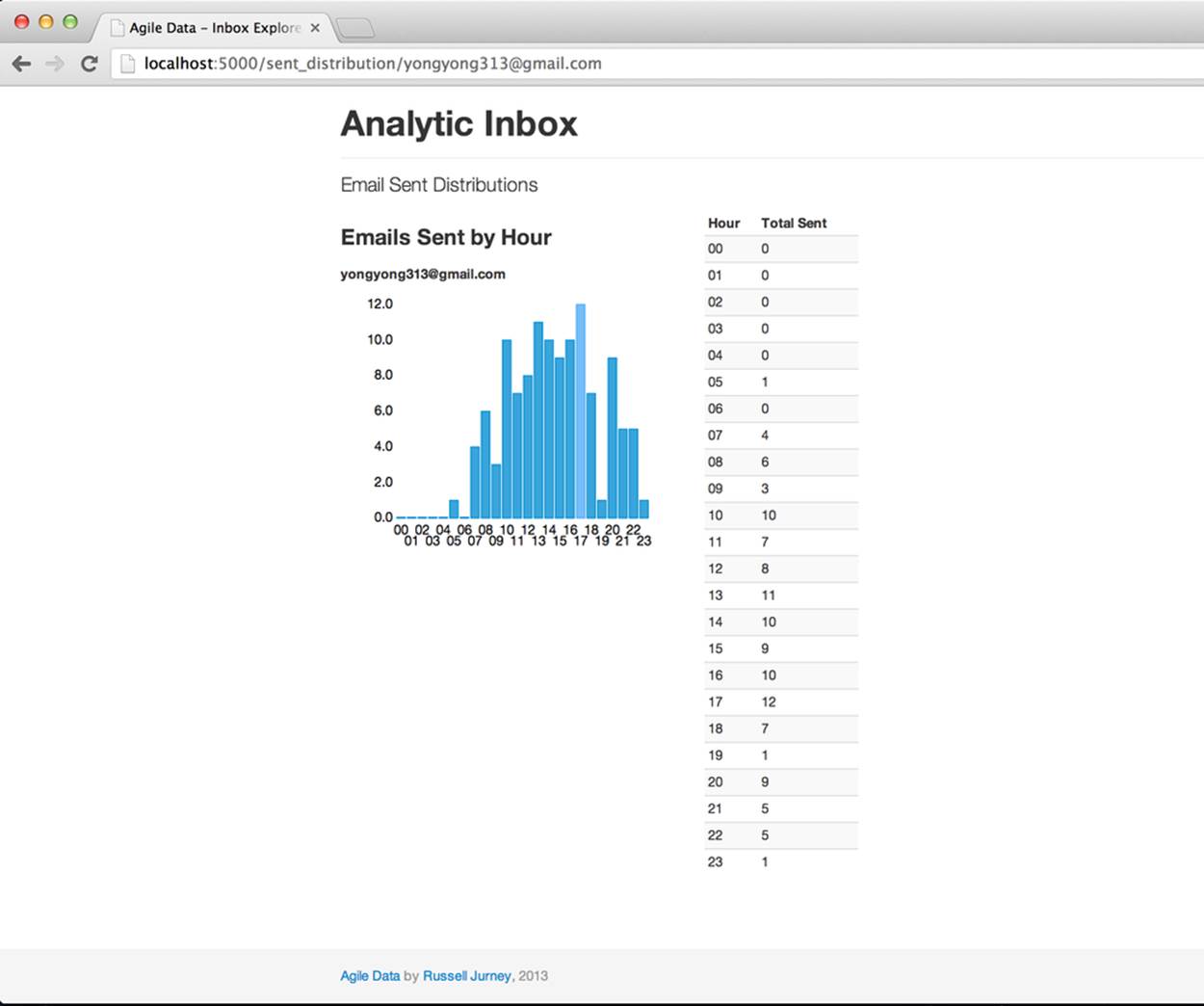
Figure 6-3. Histogram of emails sent by hour

This chart interests me because it shows different distributions even for people in the same time zone—morning people and night people.

NOTE

When you’re choosing colors for charts, http://www.colorpicker.com/ can be very helpful.

Our goal in creating charts is to draw early adopters to our application, so a good chart is something that interests real users. Along this line, we must ask ourselves: why would someone care about this data? How can we make it personally relevant? Step one is simply displaying the data in recognizable form. Step two is to highlight an interesting feature.

Accordingly, we add a new feature. We color the mode (the most common hour to send emails) in a lighter blue to highlight its significance: email this user at this time, and he is most likely to be around to see it.

We can dynamically affect the histogram’s bars with a conditional fill function. When a bar’s value matches the maximum, shade it light blue; otherwise, set the default color (Figure 6-4).

var defaultColor = '#08C';

var modeColor = '#4CA9F5';

var maxy = d3.max(data[0]['values'], function(d) { return d.total; });

var myColor = function(d, i) {

if(d['total'] == maxy) { return modeColor; }

else { return defaultColor; }

}

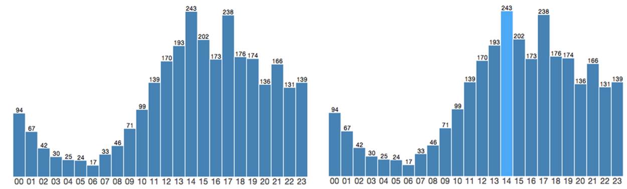
Histogram of emails sent by hour with mode highlighted

Figure 6-4. Histogram with mode highlighted

Illustrating the most likely hour a user sends email tells you when you might catch her online, and that is interesting. But to really grab the user’s attention with this chart, we need to make it personally relevant. Why should I care what time a person I know emails unless I know whether she is in sync with me?

Conclusion

In this chapter, we’ve started to tease structure from our data with charts. In doing so, we have gone further than the preceding chapter in cataloging our data assets. We’ll take what we’ve learned with us as we proceed up the data-value pyramid.

Now we move on to the next step of the data-value stack: reports.