OpenGL SuperBible: Comprehensive Tutorial and Reference, Sixth Edition (2013)

Part II: In Depth

Chapter 9. Fragment Processing and the Framebuffer

What You’ll Learn in This Chapter

• How data is passed into fragment shaders, how to control the way it’s sent there, and what to do with it once it gets there

• How to create your own framebuffers and control the format of data that they store

• How to produce more than just one output from a single fragment shader

• How to get data out of your framebuffer and into textures, buffers, and your application’s memory

This chapter is all about the back end — everything that happens after rasterization. We will take an in-depth look at some of the interesting things you can do with a fragment shader, what happens to your data once it leaves the fragment shader, and how to get it back into your application. We’re also going to look at ways to improve the quality of the images that your applications produce, from rendering in high dynamic range, to antialiasing techniques (compensating from the pixelating effect of the display) and alternative color spaces that you can render into.

Fragment Shaders

You have already been introduced to the fragment shader stage. It is the stage in the pipeline where your shader code determines the color of each fragment before it is sent for composition into the framebuffer. The fragment shader runs once per fragment, where a fragment is a virtual element of processing that might end up contributing to the final color of a pixel. Its inputs are generated by the fixed-function interpolation phase that executes as part of rasterization. By default, all members of the input blocks to the fragment shader are smoothly interpolated across the primitive being rasterized, with the endpoints of that interpolation being fed by the last stage in the front end (which may be the vertex, tessellation evaluation, or geometry shader stages). However, you have quite a bit of control over how that interpolation is performed and even whether interpolation is performed at all.

Interpolation and Storage Qualifiers

You already read about some of the storage qualifiers supported by GLSL in earlier chapters. There are a few storage qualifiers that can be used to control interpolation that you can use for advanced rendering. They include the flat and noperspective, and we quickly go over each of these here.

Disabling Interpolation

When you declare an input to your fragment shader, that input is generated, or interpolated, across the primitive being rendered. However, whenever you pass an integer from the front end to the back end, interpolation must be disabled — this is done automatically for you because OpenGL isn’t capable of smoothly interpolating integers. It is also possible to explicitly disable interpolation for floating-point fragment shader inputs. Fragment shader inputs for which interpolation has been disabled are known as flat inputs (in contrast to smooth inputs, referring to the smooth interpolation normally performed by OpenGL). To create a flat input to the fragment shader for which interpolation is not performed, declare it using the flat storage¹ qualifier, as in

1. It’s actually legal to explicitly declare floating-point fragment shader inputs with the smooth storage qualifier, although this is normally redundant as this is the default.

flat in vec4 foo;
flat in int bar;
flat in mat3 baz;

You can also apply interpolation qualifiers to input blocks, which is where the smooth qualifier comes in handy. Interpolation qualifiers applied to blocks are inherited by its members — that is, they are applied automatically to all members of the block. However, it’s possible to apply a different qualifier to individual members of the block. Thus, consider this snippet:

flat in INPUT_BLOCK
{
vec4 foo;
int bar;
smooth mat3 baz;
};

Here, foo has interpolation disabled because it inherits flat qualification from the parent block. bar is automatically flat because it is an integer. However, even though baz is a member of a block that has the flat interpolation qualifier, it is smoothly interpolated because it has the smoothinterpolation qualifier applied at the member level.

Don’t forget that while we are describing this in terms of fragment shader inputs, storage and interpolation qualifiers used on the corresponding outputs in the front end must match those used at the input of the fragment shader. This means that whatever the last stage in your front end, whether it’s a vertex, tessellation evaluation, or geometry shader, you should also declare the matching output with the flat qualifier.

When flat inputs to a fragment are in use, their value comes from only one of the vertices in a primitive. When the primitives being rendered are single points, then there is only one choice as to where to get the data. However, when the primitives being rendered are lines or triangles, either the first or last vertex in the primitive is used. The vertex from which the values for flat fragment shader inputs are taken is known as the provoking vertex, and you can decide whether that should be the first or last vertex by calling

void glProvokingVertex(GLenum provokeMode);

Here, provokeMode indicates which vertex should be used, and valid values are GL_FIRST_VERTEX_CONVENTION and GL_LAST_VERTEX_CONVENTION. The default is GL_LAST_VERTEX_CONVENTION.

Interpolating without Perspective Correction

As you have learned, OpenGL interpolates the values of fragment shader inputs across the face of primitives, such as triangles, and presents a new value to each invocation of the fragment shader. By default, the interpolation is performed smoothly in the space of the primitive being rendered. That means that if you were to look at the triangle flat on, the steps that the shader inputs take across its surface would be equal. However, OpenGL performs interpolation in screen space as it steps from pixel to pixel. Very rarely is a triangle seen directly face on, and so perspective foreshortening means that the step in each varying from pixel to pixel is not constant — that is, they are not linear in screen space. OpenGL corrects for this by using perspective-correct interpolation. To implement this, it interpolates values that are linear in screen space and uses those to derive the actual values of the shader inputs at each pixel.

Consider a texture coordinate, uv, that is to be interpolated across a triangle. Neither u nor v is linear in screen space. However (due to some math that is beyond the scope of this section), and are linear in screen space, as is (the fourth component of the fragment’s coordinate). So, what OpenGL actually interpolates is

At each pixel, it reciprocates to find w and then multiplies and by w to find u and v. This provides perspective-correct values of the interpolants to each instance of the fragment shader.

Normally, this is what you want. However, there may be times when you don’t want this. If you actually want interpolation to be carried out in screen space regardless of the orientation of the primitive, you can use the noperspective storage qualifier, like this:

noperspective out vec2 texcoord;

in the vertex shader (or whatever shader is last in the front end of your pipeline), and

noperspective in vec2 texcoord;

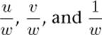
in the fragment shader, for example. The results of using perspective-correct and screen-space linear (noperspective) rendering are shown in Figure 9.1.

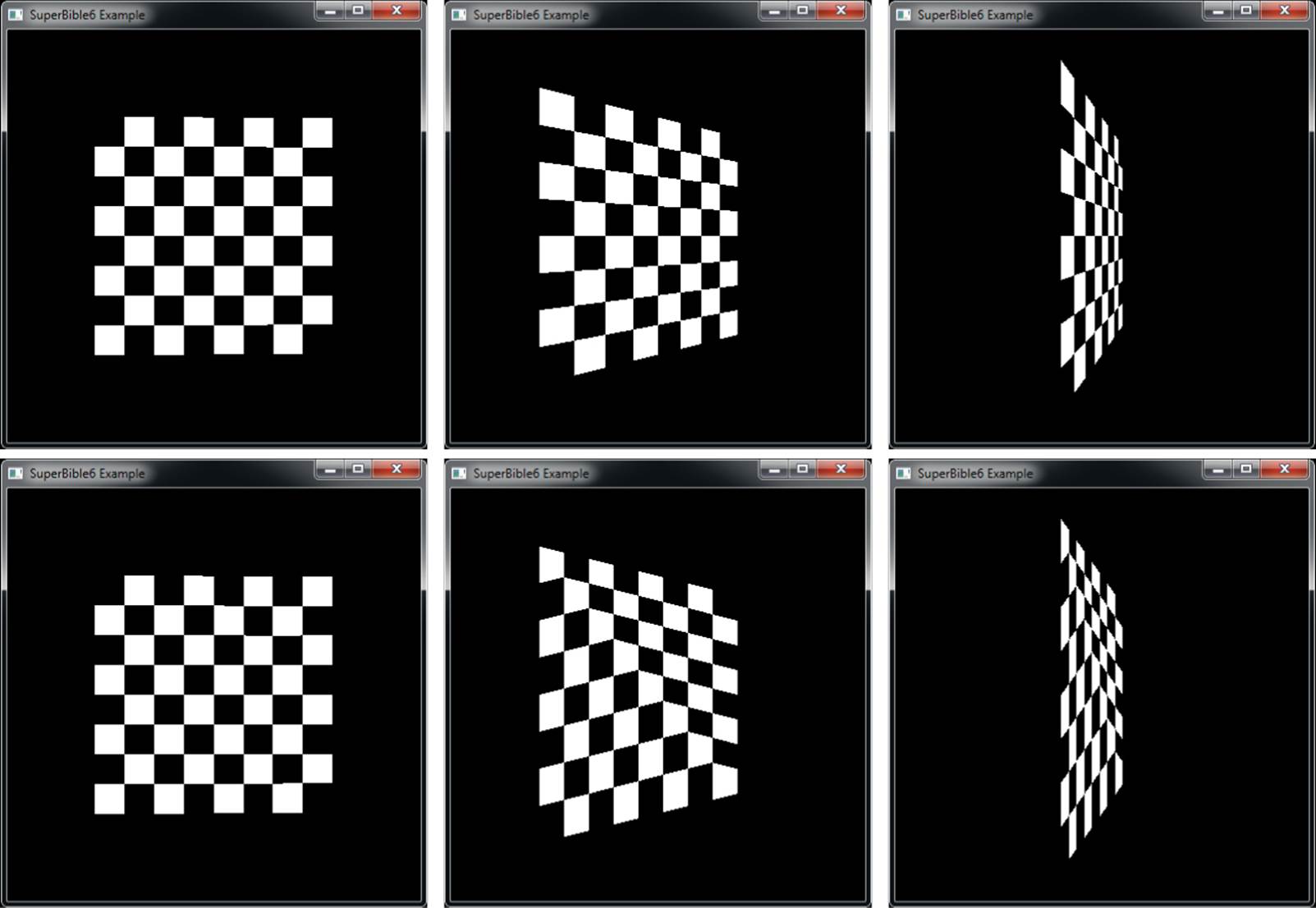
Figure 9.1: Contrasting perspective-correct and linear interpolation

The top image of Figure 9.1 shows perspective-correct interpolation applied to a pair of triangles as its angle to the viewer changes. Meanwhile, the bottom image of Figure 9.1 shows how the noperspective storage qualifier has affected the interpolation of texture coordinates. As the pair of triangles moves to a more and more oblique angle relative to the viewer, the texture becomes more and more skewed.

Per-Fragment Tests

Once the fragment shader has run, OpenGL needs to figure what do to with the fragments that are generated. Geometry has been clipped and transformed into normalized device space, and so all of the fragments that are produced by rasterization are known to be on the screen (or inside the window). However, OpenGL then performs a number of other tests on the fragment to determine if and how it should be written to the framebuffer. These tests (in logical order) are the scissor test, the stencil test, and the depth test. These are covered in pipeline order in the following section.

Scissor Testing

The scissor rectangle is an arbitrary rectangle that you can specify in screen coordinates that allows you to further clip rendering to a particular region.

Unlike the viewport, geometry is not clipped directly against the scissor rectangle, but rather individual fragments are tested against the rectangle as part of post-rasterization² processing. As with viewport rectangles, OpenGL supports an array of scissor rectangles. To set them up, you can call glScissorIndexed() or glScissorIndexedv(), whose prototypes are

2. It may be the case that some OpenGL implementations either apply scissoring at the end of the geometry stage, or in an early part of rasterization. Here, we are describing the logical OpenGL pipeline, though.

void glScissorIndexed(GLuint index,
GLint left,
GLint bottom,
GLsizei width,
GLsizei height);

void glScissorIndexedv(GLuint index,
const GLint * v);

For both functions, the index parameter specifies which scissor rectangle you want to change. The left, bottom, width, and height parameters describe a region in window coordinates that defines the scissor rectangle. For glScissorIndexedv(), the left, bottom, width, and height parameters are stored (in that order) in an array whose address is passed in v.

To select a scissor rectangle, the gl_ViewportIndex built-in output from the geometry shader is used (yes, the same one that selects the viewport). That means that given an array of viewports and an array of scissor rectangles, the same index is used for both arrays. To enable scissor testing, call

glEnable(GL_SCISSOR_TEST);

To disable it, call

glDisable(GL_SCISSOR_TEST);

The scissor test starts off disabled, so unless you need to use it, you don’t need to do anything. If we again use the shader of Listing 8.36, which employs an instanced geometry shader to write to gl_ViewportIndex, enable the scissor test, and set some scissor rectangles, we can mask off sections of rendering. Listing 9.1 shows part of the code from the multiscissor, which is to set up our scissor rectangles, and Figure 9.2 shows the result of rendering with this code.

// Turn on scissor testing
glEnable(GL_SCISSOR_TEST);

// Each rectangle will be 7/16 of the screen
int scissor_width = (7 * info.windowWidth) / 16;
int scissor_height = (7 * info.windowHeight) / 16;

// Four rectangles - lower left first...
glScissorIndexed(0, 0, 0, scissor_width, scissor_height);

// Lower right...
glScissorIndexed(1,
info.windowWidth - scissor_width, 0,
info.windowWidth - scissor_width, scissor_height);

// Upper left...
glScissorIndexed(2,
0, info.windowHeight - scissor_height,
scissor_width, scissor_height);
// Upper right...
glScissorIndexed(3,
info.windowWidth - scissor_width,
info.windowHeight - scissor_height,
scissor_width, scissor_height);

Listing 9.1: Setting up scissor rectangle arrays

Figure 9.2: Rendering with four different scissor rectangles

An important point to remember about the scissor test is that when you clear the framebuffer using glClear() or glClearBufferfv(), the first scissor rectangle is applied as well. This means that you can clear an arbitrary rectangle of the framebuffer using the scissor rectangle, but it can also lead to errors if you leave the scissor test enabled at the end of a frame and then try to clear the framebuffer ready for the next frame.

Stencil Testing

The next step in the fragment pipeline is the stencil test. Think of the stencil test as cutting out a shape in cardboard and then using that cutout to spray-paint the shape on a mural. The spray paint only hits the wall in places where the cardboard is cut out (just like a real stencil). If pixel format of the framebuffer includes a stencil buffer, you can similarly mask your draws to the framebuffer. You can enable stenciling by calling glEnable() and passing GL_STENCIL_TEST in the cap parameter. Most implementations only support stencil buffers that contain 8 bits, but some configurations may support fewer bits (or more, but this is extremely uncommon).

Your drawing commands can have a direct effect on the stencil buffer, and the value of the stencil buffer can have a direct effect on the pixels you draw. To control interactions with the stencil buffer, OpenGL provides two commands: glStencilFuncSeparate() and glStencilOpSeparate(). OpenGL lets you set both of these separately for front- and back-facing geometry. The prototypes of glStencilFuncSeparate() and glStencilOpSeparate() are

void glStencilFuncSeparate(GLenum face,
GLenum func,
GLint ref,
GLuint mask);

void glStencilOpSeparate(GLenum face,
GLenum sfail,
GLenum dpfail,
GLenum dppass);

First let’s look at glStencilFuncSeparate(), which controls the conditions under which the stencil test passes or fails. The test is applied separately for front-facing and back-facing primitives, each has its own state, and you can pass GL_FRONT, GL_BACK, or GL_FRONT_AND_BACK for face, signifying which geometry will be affected. The value of func can be any of the values in Table 9.1. These specify under what conditions geometry will pass the stencil test.

Table 9.1. Stencil Functions

The ref value is the reference used to compute the pass or fail result, and the mask parameter lets you control which bits of the reference and the buffer are compared. In pseudo-code, the operation of the stencil test is effectively implemented as

GLuint current = GetCurrentStencilContent(x, y);
if (compare(current & mask,
ref & mask,
front_facing ? front_op : back_op))
{
passed = true;
}
else
{
passed = false;
}

The next step is to tell OpenGL what to do when the stencil test passes or fails by using glStencilOpSeparate(). This function takes four parameters, with the first specifying which faces will be affected. The next three parameters control what happens after the stencil test is performed and can be any of the values in Table 9.2. The second parameter, sfail, is the action taken if the stencil test fails. The dpfail parameter specifies the action taken if the depth buffer test fails, and the final parameter, dppass, specifies what happens if the depth buffer test passes. Note that because stencil testing comes before depth testing (which we’ll get to in a moment), should the stencil test fail, the fragment is killed right there and no further processing is performed — which explains why there are only three operations here rather than four.

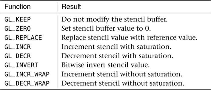
Table 9.2. Stencil Operations

So how does this actually work out? Let’s look at a simple example of typical usage shown in Listing 9.2. The first step is to clear the stencil buffer to 0 by calling glClearBufferiv() with buffer set to GL_STENCIL, drawBuffer set to 0, and value pointing to a variable containing zero. Next, a window border is drawn that may contain details such as a player’s score and statistics. Set up the stencil test to always pass with the reference value being 1 by calling glStencilFuncSeparate(). Next, tell OpenGL to replace the value in the stencil buffer only when the depth test passes by calling glStencilOpSeparate() followed by rendering the border geometry. This turns the border area pixels to 1 while the rest of the framebuffer remains at 0. Finally, set up the stencil state so that the stencil test will only pass if the stencil buffer value is 0, and then render the rest of the scene. This causes all pixels that would overwrite the border we just drew to fail the stencil test and not be drawn to the framebuffer. Listing 9.2 shows an example of how stencil can be used.

// Clear stencil buffer to 0
const GLint zero;
glClearBufferiv(GL_STENCIL, 0, &zero);

// Setup stencil state for border rendering
glStencilFuncSeparate(GL_FRONT, GL_ALWAYS, 1, 0xff);
glStencilOpSeparate(GL_FRONT, GL_KEEP, GL_ZERO, GL_REPLACE);

// Render border decorations
. . .

// Now, border decoration pixels have a stencil value of 1
// All other pixels have a stencil value of 0.

// Setup stencil state for regular rendering,
// fail if pixel would overwrite border
glStencilFuncSeparate(GL_FRONT_AND_BACK, GL_LESS, 1, 0xff);
glStencilOpSeparate(GL_FRONT, GL_KEEP, GL_KEEP, GL_KEEP);

// Render the rest of the scene, will not render over stenciled
// border content
. . .

Listing 9.2: Example stencil buffer usage, border decorations

There are also two other stencil functions: glStencilFunc() and glStencilOp(). These behave just as glStencilFuncSeparate() and glStencilOpSeparate() would if you were to set the face parameter to GL_FRONT_AND_BACK.

Controlling Updates to the Stencil Buffer

By clever manipulation of the stencil operation modes (setting them all to the same value, or judicious use of GL_KEEP, for example), you can perform some pretty flexible operations on the stencil buffer. However, beyond this, it’s possible to control updates to individual bits of the stencil buffer. The glStencilMaskSeparate() function takes a bitfield of which bits in the stencil buffer should be updated and which should be left alone. Its prototype is

void glStencilMaskSeparate(GLenum face, GLuint mask);

As with the stencil test function, there are two sets of state — one for front-facing and one for back-facing primitives. Just like glStencilFuncSeparate(), the face parameter specifies which types of primitives should be affected. The mask parameter is a bitfield that maps to the bits in the stencil buffer — if the stencil buffer has less than 32 bits (8 is the maximum supported by most current OpenGL implementations), only that many of the least significant bits of mask are used. If a mask bit is set to 1, the corresponding bit in the stencil buffer can be updated. But if the mask bit is 0, the corresponding stencil bit will not be written to. For instance, consider the following code:

GLuint mask = 0x000F;
glStencilMaskSeparate(GL_FRONT, mask);
glStencilMaskSeparate(GL_BACK, ~mask);

In the preceding example, the first call to glStencilMaskSeparate() affects front-facing primitives and enables the lower four bits of the stencil buffer for writing while leaving the rest disabled. The second call to glStencilMaskSeparate() sets the opposite mask for back-facing primitives. This essentially allows you to pack two stencil values together into an 8-bit stencil buffer — the lower four bits being used for front-facing primitives, and the upper four bits being used for back-facing primitives.

Depth Testing

After stencil operations are complete and if depth testing is enabled, OpenGL tests the depth value of a fragment against the existing content of the depth buffer. If depth writes are also enabled and the fragment has passed the depth test, the depth buffer is updated with the depth value of the fragment. If the depth test fails, the fragment is discarded and does not pass to the following fragment operations.

The input to primitive assembly is a set of vertex positions that make up primitives. Each has a z coordinate. This coordinate is scaled and biased such that the normal³ visible range of values lies between zero and one. This is the value that’s usually stored in the depth buffer. During depth testing, OpenGL reads the depth value of the fragment from the depth buffer at the current fragment’s coordinate and compares it to the generated depth value for the fragment being processed.

3. It’s possible to turn off this visibility check and consider all fragments visible, even if they lie outside the zero-to-one range that is stored in the depth buffer.

You can choose what comparison operator is used to figure out if the fragment “passed” the depth test. To set the depth comparison operator (or depth function), call glDepthFunc(), whose prototype is

void glDepthFunc(GLenum func);

Here, func is one of the available depth comparison operators. The legal values for func and what they mean are shown in Table 9.3.

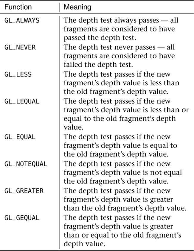
Table 9.3. Depth Comparison Functions

If the depth test is disabled, it is as if the depth test always passes (i.e., the depth function is set to GL_ALWAYS), with one exception: The depth buffer is only updated when the depth test is enabled. If you want your geometry to be written into the depth buffer unconditionally, you must enable the depth test and set the depth function to GL_ALWAYS. By default, the depth test is disabled. To turn it on, call

glEnable(GL_DEPTH_TEST);

To turn it off again, simply call glDisable() with the GL_DEPTH_TEST parameter. It is a very common mistake to disable the depth test and expect it to be updated. Again, the depth buffer is not updated unless the depth test is also enabled.

Controlling Updates of the Depth Buffer

Writes to the depth buffer can be turned on and off, regardless of the result of the depth test. Remember, the depth buffer is only updated if the depth test is turned on (although the test function can be set to GL_ALWAYS if you don’t actually need depth testing and only wish to update the depth buffer). The glDepthMask() function takes a Boolean flag that turns writes to the depth buffer on if it’s GL_TRUE and off if GL_FALSE. For example,

glDepthMask(GL_FALSE);

will turn writes to the depth buffer off, regardless of the result of the depth test. You can use this, for example, to draw geometry that should be tested against the depth buffer, but that shouldn’t update it. By default, the depth mask is set to GL_TRUE, which means you won’t need to change it if you want depth testing and writing to behave as normal.

Depth Clamping

OpenGL represents the depth of each fragment as a finite number, scaled between zero and one. A fragment with a depth of zero is intersecting the near plane (and would be jabbing you in the eye if it were real), and a fragment with a depth of one is at the farthest representable depth but not infinitely far away. To eliminate the far plane and draw things at any arbitrary distance, we would need to store arbitrarily large numbers in the depth buffer — something that’s not really possible. To get around this, OpenGL has the option to turn off clipping against the near and far planes and instead clamp the generated depth values to the range zero to one. This means that any geometry that protrudes behind the near plane or beyond the far plane will essentially be projected onto that plane.

To enable depth clamping (and simultaneously turn off clipping against the near and far planes), call

glEnable(GL_DEPTH_CLAMP);

and to disable depth clamping, call

glDisable(GL_DEPTH_CLAMP);

Figure 9.3 illustrates the effect of enabling depth clamping and drawing a primitive that intersects the near plane.

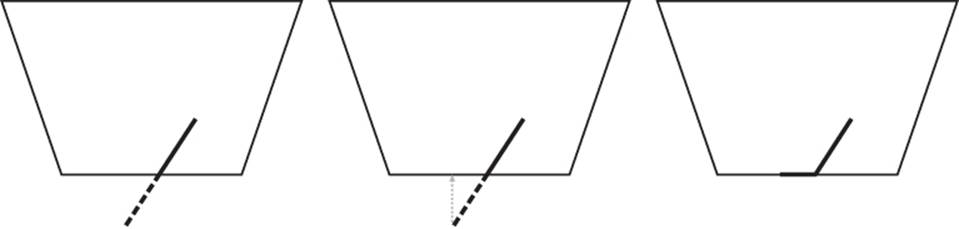
Figure 9.3: Effect of depth clamping at the near plane

It is simpler to demonstrate this in two dimensions, and so on the left of Figure 9.3, the view frustum is displayed as if we were looking straight down on it. The dark line represents the primitive that would have been clipped against the near plane, and the dotted line represents the portion of the primitive that was clipped away. When depth clamping is enabled, rather than clipping the primitive, the depth values that would have been generated outside the range zero to one are clamped into that range, effectively projecting the primitive onto the near plane (or the far plane, if the primitive would have clipped that). The center of Figure 9.3 shows this projection. What actually gets rendered is shown on the right of Figure 9.3. The dark line represents the values that eventually get written into the depth buffer. Figure 9.4 shows how this translates to a real application.

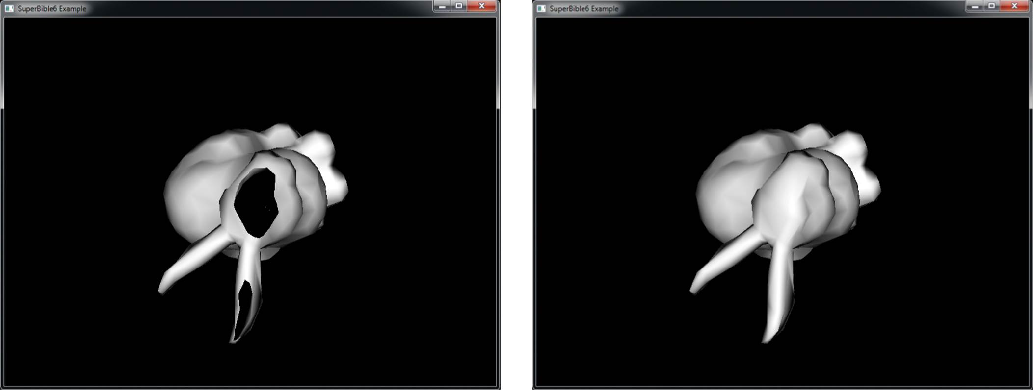
Figure 9.4: A clipped object with and without depth clamping

In the left image of Figure 9.4, the geometry has become so close to the viewer that it is partially clipped against the near plane. As a result, the portions of the polygons that would have been behind the near plane are simply not drawn, and so they leave a large hole in the model. You can see right through to the other side of the object, and the image is quite visibly incorrect. On the right of Figure 9.4, depth clamping has been enabled. As you can see, the geometry that was lost in the left image is back and fills the hole in the object. The values in the depth buffer aren’t technically correct, but this hasn’t translated to visual anomalies, and the picture produced looks better than that in the left image.

Early Testing

Logically, the depth and stencil tests occur after the fragment has been shaded, but most graphics hardware is capable of performing the test before your shader runs and avoiding the cost of executing that shader if the ownership test would fail. However, if a shader has side effects (such as directly writing to a texture) or would otherwise effect the outcome of the test, OpenGL can’t perform the tests first, and must always run your shader. Not only that, but it must always wait for the shader to finish executing before it can perform depth testing or update the stencil buffer.

One particular example of something you can do in your shader that would stop OpenGL from performing the depth test before executing it is writing to the built-in gl_FragDepth output.

The special built-in variable gl_FragDepth is available for writing an updated depth value to. If the fragment shader doesn’t write to this variable, the interpolated depth generated by OpenGL is used as the fragment’s depth value. Your fragment shader can either calculate an entirely new value for gl_FragDepth, or it can derive one from the value gl_FragCoord.z. This new value is subsequently used by OpenGL both as the reference for the depth test and as the value written to the depth buffer should the depth test pass. You can use this functionality, for example, to slightly perturb the values in the depth buffer and create physically bumpy surfaces. Of course, you’d need to shade such surfaces appropriately to make them appear bumpy, but when new objects were tested against the content of the depth buffer, the result would match the shading.

Because your shader changes the fragment’s depth value when you write to gl_FragDepth, there’s no way that OpenGL can perform the depth test before the shader runs because it doesn’t know what you’re going to put there. For this scenario, OpenGL provides some layout qualifiers that let you tell it what you plan to do with the depth value.

Now, remember that the range of values in the depth buffer is between 0.0 and 1.0, and that the depth test comparison operators include functions such as GL_LESS and GL_GREATER. Now, if you set the depth test function to GL_LESS, for example (which would pass for any fragment that is closerto the viewer than what is currently in the framebuffer), then if you only ever set gl_FragDepth to a value that is less than it would have been otherwise, then the fragment will pass the depth test regardless of whatever the shader does, and so the original test result remains valid. In this case, OpenGL now knows that it can perform the depth test before running your fragment shader, even though the logical pipeline has it running afterwards.

The layout qualifier you use to tell OpenGL what you’re going to do to depth is applied to a redeclaration of gl_FragDepth. The redeclaration of gl_FragDepth can take the form of any of the following:

layout (depth_any) out float gl_FragDepth;
layout (depth_less) out float gl_FragDepth;
layout (depth_greater) out float gl_FragDepth;
layout (depth_unchanged) out float gl_FragDepth;

If you use the depth_any layout qualifier, you’re telling OpenGL that you might write any value to gl_FragDepth. This is effectively the default — if OpenGL sees that your shader writes to gl_FragDepth, it has no idea what you did to it and assumes that the result could be anything. If you specify depth_less, you’re effectively saying that whatever you write to gl_FragDepth will result in the fragment’s depth value being less than it would have been otherwise. In this case, results from the GL_LESS and GL_LEQUAL comparison functions remain valid. Similarly, using depth_greaterindicates that your shader will only make the fragment’s depth greater than it would have been and, therefore, the result of the GL_GREATER and GL_GEQUAL tests remain valid.

The final qualifier, depth_unchanged, is somewhat unique. This tells OpenGL that whatever you do to gl_FragDepth, it’s free to assume you haven’t written anything to it that would change the result of the depth test. In the case of depth_any, depth_less, and depth_greater, although OpenGL becomes free to perform depth testing before your shader executes under certain circumstances, there are still times when it must run your shader and wait for it to finish. With depth_unchanged you are telling OpenGL that no matter what you do with the fragment’s depth value, the original result of the test remains valid. You might choose to use this if you plan to perturb the fragment’s depth slightly, but not in a way that would make it intersect any other geometry in the scene (or if you don’t care if it does).

Regardless of the layout qualifier you apply to a redeclaration of gl_FragDepth and what OpenGL decides to do about it, the value you write into gl_FragDepth will be clamped into the range 0.0 to 1.0 and then written into the depth buffer.

Color Output

The color output stage is the last part of the OpenGL pipeline before fragments are written to the framebuffer. It determines what happens to your color data between when it leaves your fragment shader and when it is finally displayed to the user.

Blending

For fragments that pass the per-fragment tests, blending is performed. Blending allows you to combine the incoming source color with the color already in the color buffer or with other constants using one of the many supported blend equations. If the buffer you are drawing to is fixed point, the incoming source colors will be clamped to 0.0 to 1.0 before any blending operations occur. Blending is enabled by calling

glEnable(GL_BLEND);

and disabled by calling

glDisable(GL_BLEND);

The blending functionality of OpenGL is powerful and highly configurable. It works by multiplying the source color (the value produced by your shader) by the source factor, then multiplying the color in the framebuffer by the destination factor, and then combining the results of these multiplications using an operation that you can choose called the blend equation.

Blend Functions

To choose the source and destination factors by which OpenGL will multiply the result of your shader and the value in the framebuffer, respectively, you can call glBlendFunc() or glBlendFuncSeparate(). glBlendFunc() lets you set the source and destination factors for all four channels of data (red, green, blue, and alpha). glBlendFuncSeparate(), on the other hand, allows you to set a source and destination factor for the red, green, and blue channels and another for the alpha channel.

glBlendFuncSeparate(GLenum srcRGB, GLenum dstRGB,
GLenum srcAlpha, GLenum dstaAlpha);

glBlendFunc(GLenum src, GLenum dst);

The possible values for these calls can be found in Table 9.4. There are four sources of data that might be used in a blending function. These are the first source color (R_s₀, G_s₀, B_s₀, and A_s₀), the second source color (R_s₁, G_s₁, B_s₁, and A_s₁), the destination color (R_d, G_d, B_d, and A_d), and the constant blending color (R_c, G_c, B_c, and A_c). The last value, the constant blending color, can be set by calling glBlendColor():

glBlendColor(GLfloat red, GLfloat green,
GLfloat blue, GLfloat alpha);

Table 9.4. Blend Functions

In addition to all of these sources, the constant values zero and one can be used as any of the product terms.

As a simple example, consider the code shown in Listing 9.3. This code clears the framebuffer to a mid-orange color, turns on blending, sets the blend color to a mid-blue color, and then draws a small cube with every possible combination of source and destination blending function.

The result of rendering with the code shown in Listing 9.3 is shown in Figure 9.5. This image is also shown in Color Plate 1 and was generated by the blendmatrix sample application.

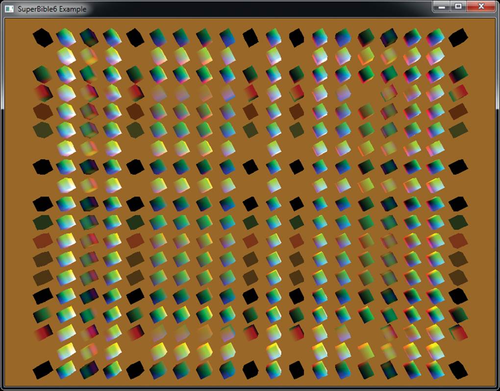
Figure 9.5: All possible combinations of blending functions

static const GLfloat orange[] = { 0.6f, 0.4f, 0.1f, 1.0f };
glClearBufferfv(GL_COLOR, 0, orange);

static const GLenum blend_func[] =
{
GL_ZERO,
GL_ONE,
GL_SRC_COLOR,
GL_ONE_MINUS_SRC_COLOR,
GL_DST_COLOR,
GL_ONE_MINUS_DST_COLOR,
GL_SRC_ALPHA,
GL_ONE_MINUS_SRC_ALPHA,
GL_DST_ALPHA,
GL_ONE_MINUS_DST_ALPHA,
GL_CONSTANT_COLOR,
GL_ONE_MINUS_CONSTANT_COLOR,
GL_CONSTANT_ALPHA,
GL_ONE_MINUS_CONSTANT_ALPHA,
GL_SRC_ALPHA_SATURATE,
GL_SRC1_COLOR,
GL_ONE_MINUS_SRC1_COLOR,
GL_SRC1_ALPHA,
GL_ONE_MINUS_SRC1_ALPHA
};
static const int num_blend_funcs = sizeof(blend_func) /
sizeof(blend_func[0]);
static const float x_scale = 20.0f / float(num_blend_funcs);
static const float y_scale = 16.0f / float(num_blend_funcs);
const float t = (float)currentTime;

glEnable(GL_BLEND);
glBlendColor(0.2f, 0.5f, 0.7f, 0.5f);
for (j = 0; j < num_blend_funcs; j++)
{
for (i = 0; i < num_blend_funcs; i++)
{
vmath::mat4 mv_matrix =
vmath::translate(9.5f - x_scale * float(i),
7.5f - y_scale * float(j),
-50.0f) *
vmath::rotate(t * -45.0f, 0.0f, 1.0f, 0.0f) *
vmath::rotate(t * -21.0f, 1.0f, 0.0f, 0.0f);

glUniformMatrix4fv(mv_location, 1, GL_FALSE, mv_matrix);

glBlendFunc(blend_func[i], blend_func[j]);

glDrawElements(GL_TRIANGLES, 36, GL_UNSIGNED_SHORT, 0);
}
}

Listing 9.3: Rendering with all blending functions

Dual-Source Blending

You may have noticed that some of the factors in Table 9.4 use source 0 colors (R_s₀, G_s₀, B_s₀, and A_s₀), and others use source 1 colors (R_s₁, G_s₁, B_s₁, and A_s₁). Your shaders can export more than one final color for a given color buffer by setting up the outputs used in your shader by assigning them indices using the index layout qualifier. An example is shown below:

layout (location = 0, index = 0) out vec4 color0;
layout (location = 0, index = 1) out vec4 color1;

Here, color0_0 will be used for the GL_SRC_COLOR factor, and color0_1 will be used for the GL_SRC1_COLOR. When you use dual source blending functions, the number of separate color buffers that you can use might be limited. You can find out how many dual output buffers are supported by querying the value of GL_MAX_DUAL_SOURCE_DRAW_BUFFERS.

Blend Equation

Once the source and destination factors have been multiplied by the source and destination colors, the two products need to be combined together. This is done using an equation that you can set by calling glBlendEquation() or glBlendEquationSeparate(). As with the blend functions, you can choose one blend equation for the red, green, and blue channels and another for the alpha channel — use glBlendEquationSeparate() to do this. If you want both equations to be the same, you can call glBlendEquation():

glBlendEquation(GLenum mode);

glBlendEquationSeparate(GLenum modeRGB,
GLenum modeAlpha);

For glBlendEquation(), the one parameter, mode, selects the same mode for all of the red, green, blue, and alpha channels. For glBlendEquationSeparate(), an equation can be chosen for the red, green, and blue channels (specified in modeRGB) and another for the alpha channel (specified inmodeAlpha). The values you pass to the two functions are shown in Table 9.5.

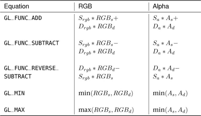
Table 9.5. Blend Equations

In Table 9.5, RGB_s represents the source red, green, and blue values; RGB_d represents the destination red, green, and blue values; A_s and A_d represent the source and destination alpha values; S_rgb and D_rgb represent the source and destination blend factors; and S_a and D_a represent the source and destination alpha factors (chosen by glBlendFunc() or glBlendFuncSeparate()).

Logical Operations

Once the pixel color is in the same format and bit depth as the framebuffer, there are two more steps that can affect the final result. The first allows you to apply a logical operation to the pixel color before it is passed on. When enabled, the effects of blending are ignored. Logic operations do not affect floating-point buffers. You can enable logic ops by calling

glEnable(GL_COLOR_LOGIC_OP);

and disable it by calling

glDisable(GL_COLOR_LOGIC_OP);

Logic operations use the values of the incoming pixel and the existing framebuffer to compute a final value. You can pick the operation that computes the final value by calling glLogicOp(). The possible options are listed in Table 9.6. The prototype of glLogicOp() is

glLogicOp(GLenum op);

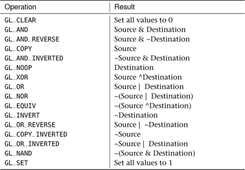
Table 9.6. Logic Operations

where op is one of the values from Table 9.6.

Logic operations are applied separately to each color channel, and operations that combine source and destination are performed bitwise on the color values. Logic ops are not commonly used in today’s graphics applications but still remain part of OpenGL because the functionality is still supported on common GPUs.

Color Masking

One of the last modifications that can be made to a fragment before it is written is masking. By now you recognize that three different types of data can be written by a fragment shader: color, depth, and stencil data. Just as you can mask off updates to the stencil and depth buffers, you can also apply a mask to the updates of the color buffer.

To mask color writes or prevent color writes from happening, you can use glColorMask() and glColorMaski(). We briefly introduced glColorMask() back in Chapter 5 where we turned on and off writing to the framebuffer. However, you don’t have to mask all color channels at once; for instance, you can choose to mask the red and green channels while permitting writes to the blue channel. Each function takes four Boolean parameters that control updates to each of the red, green, blue, and alpha channels of the color buffer. You can pass in GL_TRUE to one of these parameters to allow writes for the corresponding channel to occur, or GL_FALSE to mask these writes off. The first function, glColorMask(), allows you to mask all buffers currently enabled for rendering, while the second function, glColorMaski(), allows you to set the mask for a specific color buffer (there can be many if you’re rendering off screen). The prototypes of these two functions are

glColorMask(GLboolean red,
GLboolean green,
GLboolean blue,
GLboolean alpha);

glColorMaski(GLuint index,
GLboolean red,
GLboolean green,
GLboolean blue,
GLboolean alpha);

For both functions, red, green, blue, and alpha can be set to either GL_TRUE or GL_FALSE to determine whether the red, green, blue, or alpha channels should be written to the framebuffer. For glColorMaski(), index is the index of the color attachment to which masking should apply. Each color attachment can have its own color mask settings. So, for example, you could write only the red channel to attachment 0, only the green channel to attachment 1, and so on.

Mask Usage

Write masks can be useful for many operations. For instance, if you want to fill a shadow volume with depth information, you can mask off all color writes because only the depth information is important. Or if you want to draw a decal directly to screen space, you can disable depth writes to prevent the depth data from being polluted. The key point about masks is you can set them and immediately call your normal rendering paths, which may set up necessary buffer state and output all color, depth, and stencil data you would normally use without needing any knowledge of the mask state. You don’t have to alter your shaders to not write some value, detach some set of buffers, or change the enabled draw buffers. The rest of your rendering paths can be completely oblivious and still generate the right results.

Off-Screen Rendering

Until now, all of the rendering your programs have performed has been directed into a window, or perhaps the computer’s main display. The output of your fragment shader goes into the back buffer, which is normally owned by the operating system or window system that your application is running on, and is eventually displayed to the user. Its parameters are set when you choose a format for the rendering context. As a platform-specific operation, this means that you have little control over what the underlying storage format really is. Also, in order for the samples in this book to run on many platforms, the book’s application framework takes care of setting this up for you, hiding many of the details.

However, OpenGL includes features that allow you to set up your own framebuffer and use it to draw directly into textures. You can then use these textures later for further rendering or processing. You also have a lot of control over the format and layout of the framebuffer. For example, when you use the default framebuffer, it is implicitly sized to the size of the window or display, and rendering outside the display (if the window is obscured or dragged off the side of the screen, for example) is undefined as the corresponding pixels’ fragment shaders might not run. However, with user-supplied framebuffers, the maximum size of the textures you render to is only limited by the maximums supported by the implementation of OpenGL you’re running on, and rendering to any location in it is always defined.

User-supplied framebuffers are represented by OpenGL as framebuffer objects. As with most objects in OpenGL, each framebuffer object has a name that must be reserved before it is created — the actual object is initialized when it is first bound. So, the first thing to do is to reserve a name for a framebuffer object and bind it to the context to initialize it. To generate names for framebuffer objects, call glGenFramebuffers(), and to bind a framebuffer to the context, call glBindFramebuffer(). The prototypes of these functions are

void glGenFramebuffers(GLsizei n,
GLuint * ids);

void glBindFramebuffer(GLenum target,
GLuint framebuffer);

The glGenFramebuffers() function takes a count in n and hands you back a list of names in ids that you are able to use as framebuffer objects. The glBindFramebuffer() function makes your application-supplied framebuffer object the current framebuffer (instead of the default one). Theframebuffer is one of the names that you got from a call to glGenFramebuffers(), and target parameter will normally be GL_FRAMEBUFFER. However, it’s possible to bind two framebuffers at the same time — one for reading and one for writing.

To bind a framebuffer for reading only, set target to GL_READ_FRAMEBUFFER. Likewise, to bind a framebuffer just for rendering to, set target to GL_DRAW_FRAMEBUFFER. The framebuffer bound for drawing will be the destination for all of your rendering (including stencil and depth values used during their respective tests and colors read during blending). The framebuffer bound for reading will be the source of data if you want to read back pixel data or copy data from the framebuffer into textures, as we’ll explain shortly. Setting target to just GL_FRAMEBUFFER actually binds the object to both the read and draw framebuffer targets, and this is normally what you want.

Once you have created a framebuffer object and bound it, you can attach textures to it to serve as the storage for the rendering you’re going to do. There are three types of attachment supported by the framebuffer — the depth, stencil, and color attachments, which serve as the depth, stencil, and color buffers. To attach a texture to a framebuffer, we can call glFramebufferTexture(), whose prototype is

void glFramebufferTexture(GLenum target,
GLenum attachment,
GLuint texture,
GLint level);

For glFramebufferTexture(), target is the binding point where the framebuffer object you want to attach a texture to is bound. This should be GL_READ_FRAMEBUFFER, GL_DRAW_FRAMEBUFFER, or just GL_FRAMEBUFFER. In this case, GL_FRAMEBUFFER is considered to be equivalent toGL_DRAW_FRAMEBUFFER, and so if you use this token, OpenGL will attach the texture to the framebuffer object bound the GL_DRAW_FRAMEBUFFER target.

attachment tells OpenGL which attachment you want to attach the texture to. It can be GL_DEPTH_ATTACHMENT to attach the texture to the depth buffer attachment, or GL_STENCIL_ATTACHMENT to attach it to the stencil buffer attachment. Because there are several texture formats that include depth and stencil values packed together, OpenGL also allows you to set attachment to GL_DEPTH_STENCIL_ATTACHMENT to indicate that you want to use the same texture for both the depth and stencil buffers.

To attach a texture as the color buffer, set attachment to GL_COLOR_ATTACHMENT0. In fact, you can set attachment to GL_COLOR_ATTACHMENT1, GL_COLOR_ATTACHMENT2, and so on to attach multiple textures for rendering to. We’ll get to that momentarily, but first, we’ll look at an example of how to set up a framebuffer object for rendering to. Lastly, texture is the name of the texture you want to attach to the framebuffer, and level is the mipmap level of the texture you want to render into. Listing 9.4 shows a complete example of setting up a framebuffer object with a depth buffer and a texture to render into.

// Create a framebuffer object and bind it
glGenFramebuffers(1, &fbo);
glBindFramebuffer(GL_FRAMEBUFFER, fbo);

// Create a texture for our color buffer
glGenTextures(1, &color_texture);
glBindTexture(GL_TEXTURE_2D, color_texture);
glTexStorage2D(GL_TEXTURE_2D, 1, GL_RGBA8, 512, 512);

// We're going to read from this, but it won't have mipmaps,
// so turn off mipmaps for this texture.
glTexParameteri(GL_TEXTURE_2D, GL_TEXTURE_MIN_FILTER, GL_LINEAR);
glTexParameteri(GL_TEXTURE_2D, GL_TEXTURE_MAG_FILTER, GL_LINEAR);

// Create a texture that will be our FBO's depth buffer
glGenTextures(1, &depth_texture);
glBindTexture(GL_TEXTURE_2D, depth_texture);
glTexStorage2D(GL_TEXTURE_2D, 1, GL_DEPTH_COMPONENT32F, 512, 512);

// Now, attach the color and depth textures to the FBO
glFramebufferTexture(GL_FRAMEBUFFER,
GL_COLOR_ATTACHMENT0,
color_texture, 0);
glFramebufferTexture(GL_FRAMEBUFFER,
GL_DEPTH_ATTACHMENT,
depth_texture, 0);

// Tell OpenGL that we want to draw into the framebuffer's color
// attachment
static const GLenum draw_buffers[] = { GL_COLOR_ATTACHMENT0 };
glDrawBuffers(1, draw_buffers);

Listing 9.4: Setting up a simple framebuffer object

After this code has executed, all we need to do is call glBindFramebuffer() again and pass our newly created framebuffer object, and all rendering will be directed into the depth and color textures. Once we’re done rendering into our own framebuffer, we can use the resulting texture as a regular texture and read from it in our shaders. Listing 9.5 shows an example of doing this.

// Bind our off-screen FBO
glBindFramebuffer(GL_FRAMEBUFFER, fbo);

// Set the viewport and clear the depth and color buffers
glViewport(0, 0, 512, 512);
glClearBufferfv(GL_COLOR, 0, green);
glClearBufferfv(GL_DEPTH, 0, &one);

// Activate our first, non-textured program
glUseProgram(program1);

// Set our uniforms and draw the cube.
glUniformMatrix4fv(proj_location, 1, GL_FALSE, proj_matrix);
glUniformMatrix4fv(mv_location, 1, GL_FALSE, mv_matrix);
glDrawArrays(GL_TRIANGLES, 0, 36);

// Now return to the default framebuffer
glBindFramebuffer(GL_FRAMEBUFFER, 0);

// Reset our viewport to the window width and height, clear the
// depth and color buffers.
glViewport(0, 0, info.windowWidth, info.windowHeight);
glClearBufferfv(GL_COLOR, 0, blue);
glClearBufferfv(GL_DEPTH, 0, &one);

// Bind the texture we just rendered to for reading
glBindTexture(GL_TEXTURE_2D, color_texture);

// Activate a program that will read from the texture
glUseProgram(program2);

// Set uniforms and draw
glUniformMatrix4fv(proj_location2, 1, GL_FALSE, proj_matrix);
glUniformMatrix4fv(mv_location2, 1, GL_FALSE, mv_matrix);
glDrawArrays(GL_TRIANGLES, 0, 36);

// Unbind the texture and we're done.
glBindTexture(GL_TEXTURE_2D, 0);

Listing 9.5: Rendering to a texture

The code shown in Listing 9.5 is taken from the basicfbo sample and first binds our user-defined framebuffer, sets the viewport to the dimensions of the framebuffer, and clears the color buffer with a dark green color. It then proceeds to draw our simple cube model. This results in the cube being rendered into the texture we previously attached to the GL_COLOR_ATTACHMENT0 attachment point on the framebuffer. Next, we unbind our FBO, returning to the default framebuffer that represents our window. We render the cube again, this time with a shader that uses the texture we just rendered to. The result is that an image of the first cube we rendered is shown on each face of the second cube. Output of the program is shown in Figure 9.6.

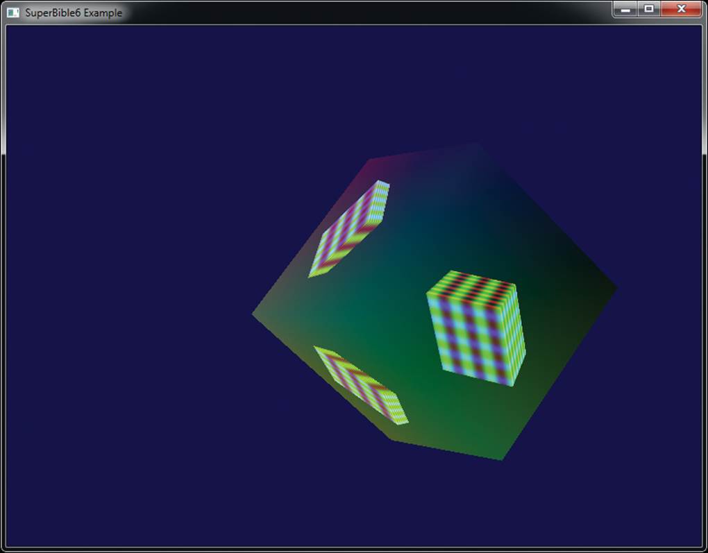
Figure 9.6: Result of rendering into a texture

Multiple Framebuffer Attachments

In the last section, we introduced the concept of user-defined framebuffers, which are also known as FBOs. An FBO allows you to render into textures that you create in your application. Because the textures are owned and allocated by OpenGL, they are decoupled from the operating or window system and so can be extremely flexible. The upper limit on their size depends only on OpenGL and not on the attached displays, for example. You also have full control over their format.

Another extremely useful feature of user-defined framebuffers is that they support multiple attachments. That is, you can attach multiple textures to a single framebuffer and render into them simultaneously with a single fragment shader. Recall that to attach your texture to your FBO, you called glFramebufferTexture() and passed GL_COLOR_ATTACHMENT0 as the attachment parameter, but we mentioned that you can also pass GL_COLOR_ATTACHMENT1, GL_COLOR_ATTACHMENT2, and so on. In fact, OpenGL supports attaching at least eight textures to a single FBO. Listing 9.6 shows an example of setting up an FBO with three color attachments.

static const GLenum draw_buffers[] =
{
GL_COLOR_ATTACHMENT0,
GL_COLOR_ATTACHMENT1,
GL_COLOR_ATTACHMENT2
};

// First, generate and bind our framebuffer object
glGenFramebuffers(1, &fbo);
glBindFramebuffer(GL_FRAMEBUFFER, fbo);

// Generate three texture names
glGenTextures(3, &color_texture[0]);

// For each one...
for (int i = 0; i < 3; i++)
{
// Bind and allocate storage for it
glBindTexture(GL_TEXTURE_2D, color_texture[i]);
glTexStorage2D(GL_TEXTURE_2D, 9, GL_RGBA8, 512, 512);

// Set its default filter parameters
glTexParameteri(GL_TEXTURE_2D,
GL_TEXTURE_MIN_FILTER, GL_LINEAR);
glTexParameteri(GL_TEXTURE_2D,
GL_TEXTURE_MAG_FILTER, GL_LINEAR);

// Attach it to our framebuffer object as color attachments
glFramebufferTexture(GL_FRAMEBUFFER,
draw_buffers[i], color_texture[i], 0);
}

// Now create a depth texture
glGenTextures(1, &depth_texture);
glBindTexture(GL_TEXTURE_2D, depth_texture);
glTexStorage2D(GL_TEXTURE_2D, 9, GL_DEPTH_COMPONENT32F, 512, 512);

// Attach the depth texture to the framebuffer
glFramebufferTexture(GL_FRAMEBUFFER, GL_DEPTH_ATTACHMENT,
depth_texture, 0);

// Set the draw buffers for the FBO to point to the color attachments
glDrawBuffers(3, draw_buffers);

Listing 9.6: Setting up an FBO with multiple attachments

To render into multiple attachments from a single fragment shader, we must declare multiple outputs in the shader and associate them with the attachment points. To do this, we use a layout qualifier to specify each output’s location, which is a term used to refer to the index of the attachment to which that output will be sent. Listing 9.7 shows an example of this.

layout (location = 0) out vec4 color0;
layout (location = 1) out vec4 color1;
layout (location = 2) out vec4 color2;

Listing 9.7: Declaring multiple outputs in a fragment shader

Once you have declared multiple outputs in your fragment shader, you can write different data into each of them and that data will be directed into the framebuffer color attachment indexed by the output’s location. Remember, the fragment shader still only executes once for each fragment produced during rasterization, and the data written to each of the shader’s outputs will be written at the same position within each of the corresponding framebuffer attachments.

Layered Rendering

In “Array Textures” in Chapter 5, we described a form of texture called the array texture, which represents a stack of 2D textures arranged as an array of layers that you can index into in a shader. It’s also possible to render into array textures by attaching them to a framebuffer object and using a geometry shader to specify which layer you want the resulting primitives to be rendered into. Listing 9.8 is taken from the gslayered sample and illustrates how to set up a framebuffer object that uses a 2D array texture as a color attachment. Such a framebuffer is known as a layered framebuffer. In addition to creating an array texture to use as a color attachment, you can create an array texture with a depth or stencil format and attach that to the depth or stencil attachment points of the framebuffer object. That texture will then become your depth or stencil buffer, allowing you to perform depth and stencil testing in a layered framebuffer.

// Create a texture for our color attachment, bind it, and allocate
// storage for it. This will be 512 × 512 with 16 layers.
GLuint color_attachment;
glGenTextures(1, &color_attachment);

glBindTexture(GL_TEXTURE_2D_ARRAY, color_attachment);
glTexStorage3D(GL_TEXTURE_2D_ARRAY, 1, GL_RGBA8, 512, 512, 16);

// Do the same thing with a depth buffer attachment.
GLuint depth_attachment;
glGenTextures(1, &depth_attachment);

glBindTexture(GL_TEXTURE_2D_ARRAY, depth_attachment);
glTexStorage3D(GL_TEXTURE_2D_ARRAY, 1, GL_DEPTH_COMPONENT, 512, 512, 16);

// Now create a framebuffer object, and bind our textures to it
GLuint fbo;
glGenFramebuffers(1, &fbo);
glBindFramebuffer(GL_FRAMEBUFFER, fbo);

glFramebufferTexture(GL_FRAMEBUFFER, GL_COLOR_ATTACHMENT0,
color_attachment, 0);
glFramebufferTexture(GL_FRAMEBUFFER, GL_DEPTH_ATTACHMENT,
depth_attachment, 0);

// Finally, tell OpenGL that we plan to render to the color
// attachment
static const GLuint draw_buffers[] = { GL_COLOR_ATTACHMENT0 };

glDrawBuffers(1, draw_buffers);

Listing 9.8: Setting up a layered framebuffer

Once you have created an array texture and attached it to a framebuffer object, you can then render into it as normal. If you don’t use a geometry shader, all rendering goes into the first layer of the array — the slice at index zero. However, if you wish to render into a different layer, you will need to write a geometry shader. In the geometry shader, the built-in variable gl_Layer is available as an output. When you write a value into gl_Layer, that value will be used to index into the layered framebuffer to select the layer of the attachments to render into. Listing 9.9 shows a simple geometry shader that renders 16 copies of the incoming geometry, each with a different model-view matrix, into an array texture and passes a per-invocation color along to the fragment shader.

#version 430 core

// 16 invocations of the geometry shader, triangles in
// and triangles out
layout (invocations = 16, triangles) in;
layout (triangle_strip, max_vertices = 3) out;

in VS_OUT
{
vec4 color;
vec3 normal;
} gs_in[];

out GS_OUT
{
vec4 color;
vec3 normal;
} gs_out;

// Declare a uniform block with one projection matrix and
// 16 model-view matrices
layout (binding = 0) uniform BLOCK
{
mat4 proj_matrix;
mat4 mv_matrix[16];
};

void main(void)
{
int i;

// 16 colors to render our geometry
const vec4 colors[16] = vec4[16](
vec4(0.0, 0.0, 1.0, 1.0), vec4(0.0, 1.0, 0.0, 1.0),
vec4(0.0, 1.0, 1.0, 1.0), vec4(1.0, 0.0, 1.0, 1.0),
vec4(1.0, 1.0, 0.0, 1.0), vec4(1.0, 1.0, 1.0, 1.0),
vec4(0.0, 0.0, 0.5, 1.0), vec4(0.0, 0.5, 0.0, 1.0),
vec4(0.0, 0.5, 0.5, 1.0), vec4(0.5, 0.0, 0.0, 1.0),
vec4(0.5, 0.0, 0.5, 1.0), vec4(0.5, 0.5, 0.0, 1.0),
vec4(0.5, 0.5, 0.5, 1.0), vec4(1.0, 0.5, 0.5, 1.0),
vec4(0.5, 1.0, 0.5, 1.0), vec4(0.5, 0.5, 1.0, 1.0)
);

for (i = 0; i < gl_in.length(); i++)
{
// Pass through all the geometry
gs_out.color = colors[gl_InvocationID];
gs_out.normal = mat3(mv_matrix[gl_InvocationID]) * gs_in[i].normal;
gl_Position = proj_matrix *
mv_matrix[gl_InvocationID] *
gl_in[i].gl_Position;
// Assign gl_InvocationID to gl_Layer to direct rendering
// to the appropriate layer
gl_Layer = gl_InvocationID;
EmitVertex();
}
EndPrimitive();
}

Listing 9.9: Layered rendering using a geometry shader

The result of running the geometry shader shown in Listing 9.9 is that we have an array texture with a different view of a model in each slice. Obviously, we can’t directly display the contents of an array texture, so we must now use our texture as the source of data in another shader. The vertex shader in Listing 9.10, along with the corresponding fragment shader in Listing 9.11, displays the contents of an array texture.

#version 430 core

out VS_OUT
{
vec3 tc;
} vs_out;

void main(void)
{
int vid = gl_VertexID;
int iid = gl_InstanceID;
float inst_x = float(iid % 4) / 2.0;
float inst_y = float(iid >> 2) / 2.0;

const vec4 vertices[] = vec4[](vec4(-0.5, -0.5, 0.0, 1.0),
vec4( 0.5, -0.5, 0.0, 1.0),
vec4( 0.5, 0.5, 0.0, 1.0),
vec4(-0.5, 0.5, 0.0, 1.0));

vec4 offs = vec4(inst_x - 0.75, inst_y - 0.75, 0.0, 0.0);

gl_Position = vertices[vid] *
vec4(0.25, 0.25, 1.0, 1.0) + offs;
vs_out.tc = vec3(vertices[vid].xy + vec2(0.5), float(iid));
}

Listing 9.10: Displaying an array texture — vertex shader

#version 430 core

layout (binding = 0) uniform sampler2DArray tex_array;

layout (location = 0) out vec4 color;

in VS_OUT
{
vec3 tc;
} fs_in;

void main(void)
{
color = texture(tex_array, fs_in.tc);
}

Listing 9.11: Displaying an array texture — fragment shader

The vertex shader in Listing 9.10 simply produces a quad based on the vertex index. In addition, it offsets the quad using a function of the instance index such that rendering 16 instances will produce a 4 × 4 grid of quads. Finally, it also produces a texture coordinate using the x and ycomponents of the vertex along with the instance index as the third component. Because we will use this to fetch from an array texture, this third component will select the layer. The fragment shader in Listing 9.11 simply reads from the array texture using the supplied texture coordinates and sends the result to the color buffer.

The result of the program is shown in Figure 9.7. As you can see, 16 copies of the torus have been rendered, each with a different color and orientation. Each of the 16 copies is then drawn into the window by reading from a separate layer of the array texture.

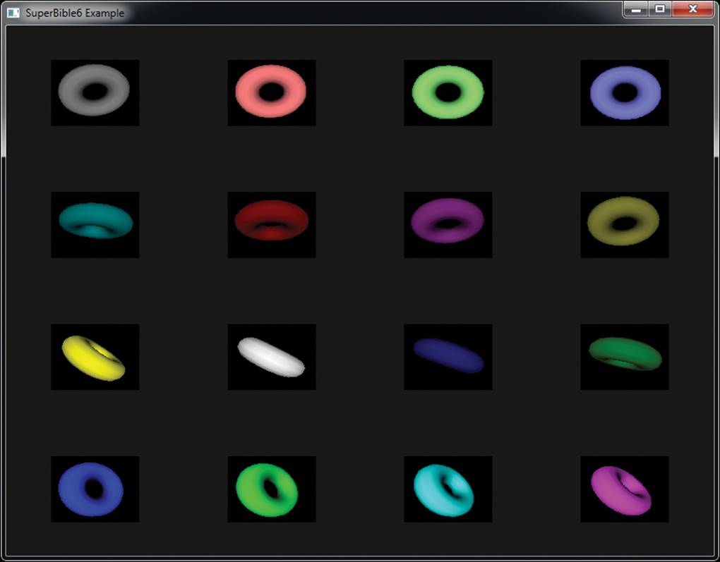
Figure 9.7: Result of the layered rendering example

Rendering into a 3D texture works in almost exactly the same way. You simply attach the whole 3D texture to a framebuffer object as one of its color attachments and then set the gl_Layer output as normal. The value written to gl_Layer becomes the z coordinate of the slice within the 3D texture where data produced by the fragment shader will be written. It’s even possible to render into multiple slices of the same texture (array or 3D) at the same. To do this, call glFramebufferTextureLayer(), whose prototype is

void glFramebufferTextureLayer(GLenum target,
GLenum attachment,
GLuint texture,
GLint level,
GLint layer);

The glFramebufferTextureLayer() function works just like glFramebufferTexture(), except that it takes one additional parameter, layer, which specifies the layer of the texture that you wish to attach to the framebuffer. For instance, the code in Listing 9.12 creates a 2D array texture with eight layers and attaches each of the layers to the corresponding color attachment of a framebuffer object.

GLuint tex;
glGenTextures(1, &tex);
glBindTexture(GL_TEXTURE_2D_ARRAY, tex);
glTexStorage3D(GL_TEXTURE_2D_ARRAY, 1, GL_RGBA8, 256, 256, 8);

GLuint fbo;
glGenFramebuffers(1, &fbo);
glBindFramebuffer(GL_FRAMEBUFFER, fbo);

int i;
for (i = 0; i < 8; i++)
{
glFramebufferTextureLayer(GL_FRAMEBUFFER,
GL_COLOR_ATTACHMENT0 + i,
tex,
0,
i);
}

static const GLenum draw_buffers[] =
{
GL_COLOR_ATTACHMENT0, GL_COLOR_ATTACHMENT1,
GL_COLOR_ATTACHMENT2, GL_COLOR_ATTACHMENT3,
GL_COLOR_ATTACHMENT4, GL_COLOR_ATTACHMENT5,
GL_COLOR_ATTACHMENT6, GL_COLOR_ATTACHMENT7
};
glDrawBuffers(8, &draw_buffers[0]);

Listing 9.12: Attaching texture layers to a framebuffer

Now, when you render into the framebuffer created in Listing 9.12, your fragment shader can have up to eight outputs, and each will be written to a different layer of the texture.

Rendering to Cube Maps

As far as OpenGL is concerned, a cube map is really a special case of an array texture. A single cube map is just an array of six slices, and a cube map array texture is an array of an integer multiple of six slices. You attach a cube map texture to a framebuffer object in exactly the same way as shown in Listing 9.8, except that rather than creating a 2D array texture, you create a cube map texture. The cube map has six faces, which are known as positive and negative x, positive and negative y, and positive and negative z, and they appear in that order in the array texture. When you write 0 into gl_Layer in your geometry shader, rendering will go to the positive x face of the cube map. Writing 1 into gl_Layer sends output to the negative x face, writing 2 sends output to the positive y face, and so on, until eventually, writing 5 sends output to the negative z face.

If you create a cube map array texture and attach it to a framebuffer object, writing to the first six layers will render into the first cube, writing the next six layers will write into the second cube, and so on. So, if you set gl_Layer to 6, you will write to the positive x face of the second cube in the array. If you set gl_Layer to 1234, you will render into the positive z face of the 205th face.

Just as with 2D array textures, it’s also possible to attach individual faces of a cube map to the various attachment points of a single framebuffer object. In this case, we use the glFramebufferTexture2D() function, whose prototype is

void glFramebufferTexture2D(GLenum target,
GLenum attachment,
GLenum textarget,
GLuint texture,
GLint level);

Again, this function works just like glFramebufferTexture(), except that it has one additional parameter, textarget. This can be set to specify which face of the cube map you want to attach to the attachment. To attach the cube map’s positive x face, set this to GL_CUBE_MAP_POSITIVE_X; for the negative x face, set it to GL_CUBE_MAP_NEGATIVE_X. Similar tokens are available for the y and z faces, too. Using this, you could bind all of the faces of a single cube map⁴ to the attachment points on a single framebuffer and render into all of them at the same time.

4. While this is certainly possible, rendering the same thing to all faces of a cube map has limited utility.

Framebuffer Completeness

Before we can finish up with framebuffer objects, there is one last important topic. Just because you are happy with the way you set up your FBO doesn’t mean your OpenGL implementation is ready to render. The only way to find out if your FBO is set up correctly and in a way that the implementation can use it is to check for framebuffer completeness. Framebuffer completeness is similar in concept to texture completeness. If a texture doesn’t have all required mipmap levels specified with the right sizes, formats, and so on, that texture is incomplete and can’t be used.

There are two categories of completeness: attachment completeness and whole framebuffer completeness.

Attachment Completeness

Each attachment point of an FBO must meet certain criteria to be considered complete. If any attachment point is incomplete, the whole framebuffer will also be incomplete. Some of the cases that cause an attachment to be incomplete are

• No image is associated with the attached object.

• Width or height of zero for attached image.

• A non-color renderable format is attached to a color attachment.

• A non-depth renderable format is attached to a depth attachment.

• A non-stencil renderable format is attached to a stencil attachment.

Whole Framebuffer Completeness

Not only does each attachment point have to be valid and meet certain criteria, but the framebuffer object as a whole must also be complete. The default framebuffer, if one exists, will always be complete. Common cases for the whole framebuffer being incomplete are

• glDrawBuffers() has mapped an output to an FBO attachment where no image is attached.

• The combination of internal formats is not supported by the OpenGL driver.

Checking the Framebuffer

When you think you are finished setting up an FBO, you can check to see whether it is complete by calling

GLenum fboStatus = glCheckFramebufferStatus(GL_DRAW_FRAMEBUFFER);

If glCheckFramebufferStatus() returns GL_FRAMEBUFFER_COMPLETE, all is well, and you may use the FBO. The return value of glCheckFramebufferStatus() provides clues to what might be wrong if the framebuffer is not complete. Table 9.7 describes all possible return conditions and what they mean.

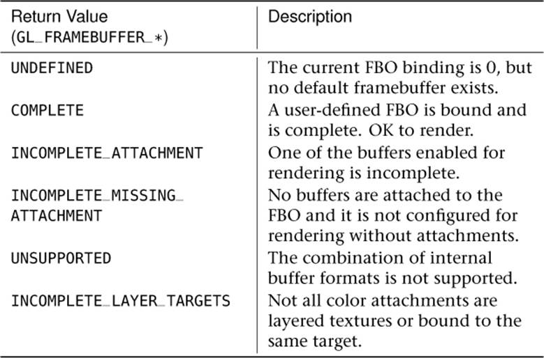
Table 9.7. Framebuffer Completeness Return Values

Many of these return values are helpful when debugging an application but are less useful after an application has shipped. Nonetheless, the first sample application checks to make sure none of these conditions occurred. It pays to do this check in applications that use FBOs, making sure your use case hasn’t hit some implementation-dependent limitation. An example of how this might look is shown in Listing 9.13.

GLenum fboStatus = glCheckFramebufferStatus(GL_DRAW_FRAMEBUFFER);
if(fboStatus != GL_FRAMEBUFFER_COMPLETE)
{
switch (fboStatus)
{
case GL_FRAMEBUFFER_UNDEFINED:
// Oops, no window exists?
break;
case GL_FRAMEBUFFER_INCOMPLETE_ATTACHMENT:
// Check the status of each attachment
break;
case GL_FRAMEBUFFER_INCOMPLETE_MISSING_ATTACHMENT:
// Attach at least one buffer to the FBO
break;
case GL_FRAMEBUFFER_INCOMPLETE_DRAW_BUFFER:
// Check that all attachments enabled via
// glDrawBuffers exist in FBO
case GL_FRAMEBUFFER_INCOMPLETE_READ_BUFFER:
// Check that the buffer specified via
// glReadBuffer exists in FBO
break;
case GL_FRAMEBUFFER_UNSUPPORTED:
// Reconsider formats used for attached buffers
break;
case GL_FRAMEBUFFER_INCOMPLETE_MULTISAMPLE:
// Make sure the number of samples for each
// attachment is the same
break;
case GL_FRAMEBUFFER_INCOMPLETE_LAYER_TARGETS:
// Make sure the number of layers for each
// attachment is the same
break;
}
}

Listing 9.13: Checking completeness of a framebuffer object

If you attempt to perform any command that reads from or writes to the framebuffer while an incomplete FBO is bound, the command simply returns after throwing the error GL_INVALID_FRAMEBUFFER_OPERATION, retrievable by calling glGetError().

Read Framebuffers Need to Be Complete, Too!

In the previous examples, we test the FBO attached to the draw buffer binding point, GL_DRAW_FRAMEBUFFER. But a framebuffer attached to GL_READ_FRAMEBUFFER also has to be attachment complete and whole framebuffer complete for reads to work. Because only one read buffer can be enabled at a time, making sure an FBO is complete for reading is a little easier.

Rendering in Stereo

Most⁵ human beings have two eyes. We use these two eyes to help us judge distance by providing parallax shift — a slight difference between the images our two eyes see. There are many depth queues, including depth from focus, from differences in lighting and the relative movement of objects as we move our point of view. OpenGL is able to produce pairs of images that, depending on the display device used, can be presented separately to your two eyes and increase the sense of depth of the image. There are plenty of display devices available including binocular displays (devices with a separate physical display for each eye), shutter and polarized displays that require glasses to view, and autostereoscopic displays that don’t require that you put anything on your face. OpenGL doesn’t really care about how the image is displayed, only that you wish to render two views of the scene — one for the left eye and one for the right.

5. Those readers with less than two eyes may wish to skip to the next section.

To display images in stereo requires some cooperation from the windowing or operating system, and therefore the mechanism to create a stereo display is platform specific. The gory details of this are covered for a number of platforms in Chapter 14. For now, we can use the facilities provided by the sb6 application framework to create our stereo window for us. In your application, you can override sb6::application::init, call the base class function, and then set info.flags.stereo to 1 as shown in Listing 9.14. Because some OpenGL implementations may require your application to cover the whole display (which is known as full-screen rendering), you can also set the info.flags.fullscreen flag in your init function to make the application use a full-screen window.

void my_application::init()
{
info.flags.stereo = 1;
info.flags.fullscreen = 1; // Set this if your OpenGL
// implementation requires
// fullscreen for stereo rendering.
}

Listing 9.14: Creating a stereo window

Remember, not all displays support stereo output, and not all OpenGL implementations will allow you to create a stereo window. However, if you have access to the necessary display and OpenGL implementation, you should have a window that runs in stereo. Now we need to render into it. The simplest way to render in stereo is to simply draw the entire scene twice. Before rendering into the left eye image, call

glDrawBuffer(GL_BACK_LEFT);

When you want to render into the right eye image, call

glDrawBuffer(GL_BACK_RIGHT);

In order to produce a pair of images with a compelling depth effect, you need to construct transformation matrices representing the views observed by the left and right eyes. Remember, our model matrix transforms our model into world space, and world space is global, applying the same way regardless of the viewer. However, the view matrix essentially transforms the world into the frame of the viewer. As the viewer is in a different location for each of the eyes, the view matrix must be different for each of the two eyes. Therefore, when we render to the left view, we use the left view matrix, and when we’re rendering to the right view, we use the right view matrix.

The simplest form of stereo view matrix pairs simply translates the left and right views away from each other on the horizontal axis. Optionally, you can also rotate the view matrices inwards towards the center of view. Alternatively, you can use the vmath::lookat function to generate your view matrices for you. Simply place your eye at the left eye location (slightly left of the viewer position) and the center of the object of interest to create the left view matrix, and then do the same with the right eye position to create the right view matrix. Listing 9.15 shows how this is done.

void my_application::render(double currentTime)
{
static const vmath::vec3 origin(0.0f);
static const vmath::vec3 up_vector(0.0f, 1.0f, 0.0f);
static const vmath::vec3 eye_separation(0.01f, 0.0f, 0.0f);

vmath::mat4 left_view_matrix =
vmath::lookat(eye_location - eye_separation,
origin,
up_vector);

vmath::mat4 right_view_matrix =
vmath::lookat(eye_location + eye_separation,
origin,
up_vector);

static const GLfloat black[] = { 0.0f, 0.0f ,0.0f, 0.0f };
static const GLfloat one = 1.0f;

// Setting the draw buffer to GL_BACK ends up drawing in
// both the back left and back right buffers. Clear both
glDrawBuffer(GL_BACK);
glClearBufferfv(GL_COLOR, 0, black);
glClearBufferfv(GL_DEPTH, 0, &one);

// Now, set the draw buffer to back left
glDrawBuffer(GL_BACK_LEFT);

// Set our left model-view matrix product
glUniformMatrix4fv(model_view_loc, 1,
left_view_matrix * model_matrix);

// Draw the scene
draw_scene();

// Set the draw buffer to back right
glDrawBuffer(GL_BACK_RIGHT);

// Set the right model-view matrix product
glUniformMatrix4fv(model_view_loc, 1,
right_view_matrix * model_matrix);

// Draw the scene... again.
draw_scene();
}

Listing 9.15: Drawing into a stereo window

Clearly, the code in Listing 9.15 renders the entire scene twice. Depending on the complexity of your scene, that could be very, very expensive — literally doubling the cost of rendering the scene. One possible tactic is to switch between the GL_BACK_LEFT and GL_BACK_RIGHT draw buffers between each and every object in your scene. This can mean that updates to state (such as binding textures or changing the current program) can be performed only once, but changing the draw buffer can be as expensive as any other state-changing function. As we learned earlier in the chapter, though, it’s possible to render into more than one buffer at a time by outputting two vectors from your fragment shader. In fact, consider what would happen if you used a fragment shader with two outputs and then call

static const GLenum buffers[] = { GL_BACK_LEFT, GL_BACK_RIGHT }
glDrawBuffers(2, buffers);

After this, the first output of your fragment shader will be written to the left eye buffer, and the second will be written to the right eye buffer. This is great! Now we can render both eyes at the same time! Well, not so fast. Remember, even though the fragment shader can output to a number of different draw buffers, the location within each of those buffers will be the same. How do we draw a different image into each of the buffers?

What we can do is use a geometry shader to render into a layered framebuffer with two layers, one for the left eye and one for the right eye. We will use geometry shader instancing to run the geometry shader twice, and write the invocation index into the layer to direct the two copies of the data into the two layers of the framebuffer. In each invocation of the geometry shader, we can select one of two model-view matrices and essentially perform all of the work of the vertex shader in the geometry shader. Once we’re done rendering the whole scene, the framebuffer’s two layers will contain the left and right eye images. All that is needed now is to render a full-screen quad with a fragment shader that reads from the two layers of the array texture and writes the result into its two outputs, which are directed into the left and right eye views.

Listing 9.16 shows the simple geometry shader that we’ll use in our application to render both views of our stereo scene in a single pass.

#version 430 core

layout (triangles, invocations = 2) in;
layout (triangle_strip, max_vertices = 3) out;

uniform matrices
{
mat4 model_matrix;
mat4 view_matrix[2];
mat4 projection_matrix;
};

in VS_OUT
{
vec4 color;
vec3 normal;
vec2 texture_coord;
} gs_in[];

out GS_OUT
{
vec4 color;
vec3 normal;
vec2 texture_coord;
} gs_out;

void main(void)
{
// Calculate a model-view matrix for the current eye
mat4 model_view_matrix = view_matrix[gl_InvocationID] *
model_matrix;

for (int i = 0; i < gl_in.length(); i++)
{
// Output layer is invocation ID
gl_Layer = gl_InvocationID;
// Multiply by the model matrix, view matrix for the
// appropriate eye and then the projection matrix.
gl_Position = projection_matrix *
model_view_matrix *
gl_in[i].gl_Position;
gs_out.color = gs_in[i].color;
// Don't forget to transform the normals...
gs_out.normal = mat3(model_view_matrix) * gs_in[i].normal;
gs_out.texcoord = gs_in[i].texcoord;
EmitVertex();
}

EndPrimitive();
}

Listing 9.16: Rendering to two layers with a geometry shader

Now that we’ve rendered our scene into our layered framebuffer, we can attach the underlying array texture and draw a full-screen quad to copy the result into the left and right back buffers with a single shader. Such a shader is shown in Listing 9.17.

#version 430 core

layout (location = 0) out vec4 color_left;
layout (location = 1) out vec4 color_right;

in vec2 tex_coord;

uniform sampler2DArray back_buffer;

void main(void)
{
color_left = texture(back_buffer, vec3(tex_coord, 0.0));
color_right = texture(back_buffer, vec3(tex_coord, 1.0));
}

Listing 9.17: Copying from an array texture to a stereo back buffer

A photograph running this application is shown in Figure 9.8. A photograph is necessary here as a screenshot would not show both of the images in the stereo pair. However, the double image produced by stereo rendering is clearly visible in the photograph.

Figure 9.8: Result of stereo rendering to a stereo display

Antialiasing

Aliasing is an artifact of under-sampling data. It is a term commonly used in signal processing fields. When aliasing occurs in an audio signal, it can be heard as a high-pitched whining or crunching sound. You may have noticed this in old video games, musical greeting cards, or children’s toys that often include low-cost playback devices. Aliasing occurs when the rate at which a signal is sampled (the sampling rate) is too low for the content of that signal. The rate at which a sample must be sampled in order to preserve (most of) its content is known as the Nyquist rate, and is twice the frequency of the highest frequency component present in the signal to be captured. In image terms, aliasing manifests as jagged edges wherever there is sharp contrast. These edges are sometimes referred to as jaggies.

There are two main approaches to deal with aliasing. The first is filtering, which removes high-frequency content from the signal before or during sampling. The second is increasing the sampling rate, which allows the higher frequency content to be recorded. The additional samples captured can then be processed for storage or reproduction. Methods for reducing or eliminating aliasing are known as antialiasing techniques. OpenGL includes a number of ways to apply antialiasing to your scene. These include filtering geometry as it is rendered, and various forms of over-sampling.

Antialiasing by Filtering

The first and simplest way to deal with the aliasing problem is to filter primitives as they are drawn. To do this, OpenGL calculates the amount of a pixel that is covered by a primitive (point, line, or triangle) and uses it to generate an alpha value for each fragment. This alpha value is multiplied by the alpha value of the fragment produced by your shader and so has an effect on blending when either the source or destination blend factor includes the source alpha term. Now, as fragments are drawn to the screen, they are blended with its existing content using a function of the pixel coverage.

To turn on this form of antialiasing, we need to do two things. First, we need to enable blending and choose an appropriate blending function. Second, we need to enable GL_LINE_SMOOTH to apply antialiasing to lines and GL_POLYGON_SMOOTH to apply antialiasing to triangles. Figure 9.9 shows the result of doing this.

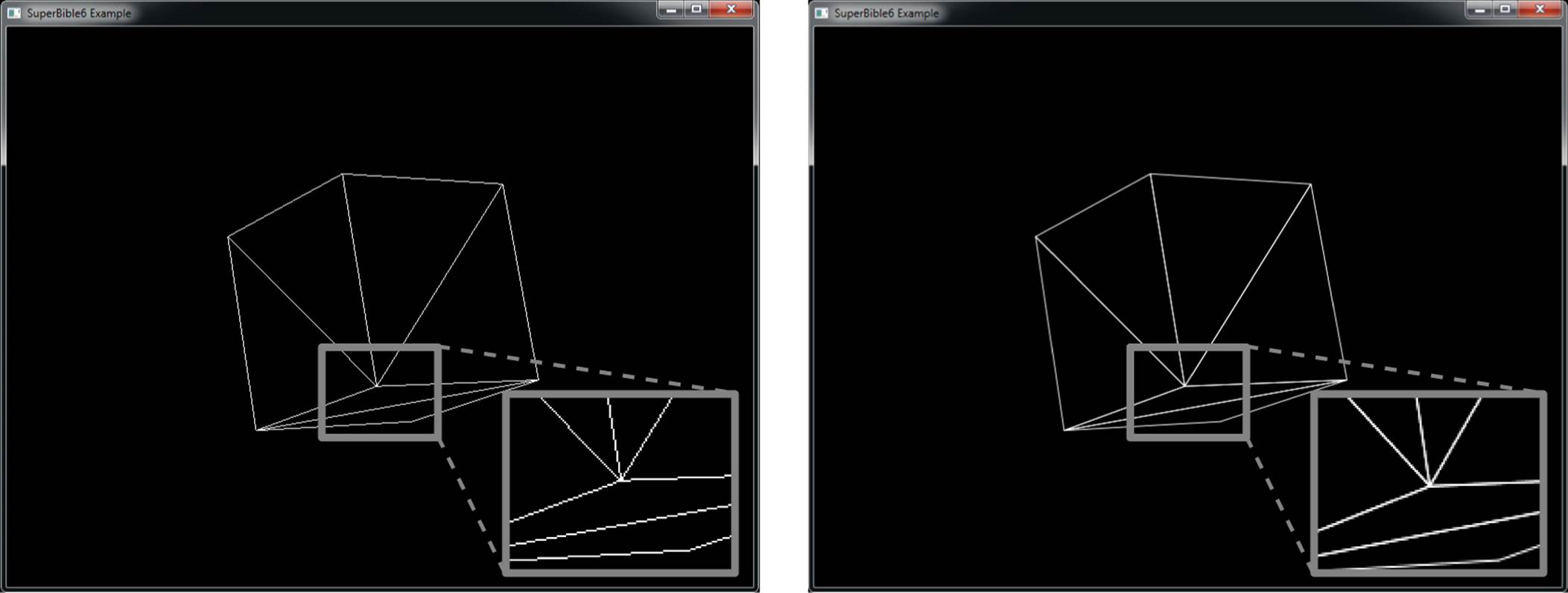
Figure 9.9: Antialiasing using line smoothing

On the left of Figure 9.9, we have drawn our spinning cube in line mode and zoomed in on a section of the image where a number of edges join each other. In the inset, the aliasing artifacts are clearly visible — notice the jagged edges. In the image on the right of Figure 9.9, line smoothingand blending are enabled, but the scene is otherwise unchanged. Notice how the lines appear much smoother and the jagged edges are much reduced. Zooming into the inset, we see that the lines have been blurred slightly. This is the effect of filtering that is produced by calculating the coverage of the lines and using it to blend them with the background color. The code to set up antialiasing and blending in order to render the image is shown in Listing 9.18.

glEnable(GL_BLEND);
glBlendFunc(GL_SRC_ALPHA, GL_ONE_MINUS_SRC_ALPHA);
glEnable(GL_LINE_SMOOTH);

Listing 9.18: Turning on line smoothing

Listing 9.18 seems pretty simple, doesn’t it? Surely, if it’s that simple, we should be able to turn this on for any geometry we like and everything will just look better. Well, no, that’s not really true. This form of antialiasing only works in limited cases like the one shown in Figure 9.9. Take a look at the images in Figure 9.10.

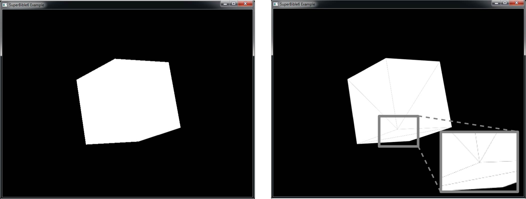
Figure 9.10: Antialiasing using polygon smoothing

The left image in Figure 9.10 shows our cube rendered in solid white. You can see that the jaggies in the middle where the individual triangles abut aren’t visible, but on the edges of the cube, we can see the aliasing effect quite clearly. In the image on the right of Figure 9.10, we have turned on polygon smoothing using code almost identical to that of Listing 9.18, only substituting GL_POLYGON_SMOOTH for GL_LINE_SMOOTH. Now, although the edges of the cube are smoothed and the jaggies are mostly gone, what happened to the interior edges? They have become visible!

Consider what happens when the edge between two adjoining triangles cuts exactly halfway through the middle of a pixel. First, our application clears the framebuffer to black, and then our first white triangle hits that pixel. OpenGL calculates that half the pixel is covered by the triangle, and uses an alpha value of 0.5 in the blending equation. This mixes half and half white and black, producing a mid-gray pixel. Next, our second, adjacent triangle comes along and covers the other half of the pixel. Again, OpenGL figures that half the pixel is covered by the new triangle and mixes the white of the triangle with the existing framebuffer content... except now the framebuffer is 50% gray! Mixing white and 50% gray produces 75% gray, which is the color we see in the lines between the triangles.

Ultimately, whenever a polygon edge cuts part of the way through a pixel and is written to the screen, OpenGL has no way to know which part is already covered and which part is not. This leads to artifacts like those seen in Figure 9.10. Another significant issue with this method is that there is only one depth value for each pixel, which means that if a triangle pokes into a not-yet-covered part of a pixel, it may still fail the depth test and not contribute at all if there’s already a closer triangle covering a different part of that same pixel.

To circumvent these problems, we need more advanced antialiasing methods, all of which include increasing the sample count.

Multi-sample Antialiasing

To increase the sample rate of the image, OpenGL supports storing multiple samples for every pixel on the screen. This technique is known as multi-sample antialiasing or MSAA. Rather than sampling each primitive only once, OpenGL will sample the primitive at multiple locations within the pixel and, if any are hit, run your shader. Whatever color your shader produces is written into all of the hit samples. The actual location of the samples within each pixel might be different on different OpenGL implementations. Figure 9.11 shows an example arrangement of the sample positions for 1, 2, 4, and 8 sample arrangements.

Figure 9.11: Antialiasing sample positions

Turning on MSAA for the default framebuffer is somewhat platform specific. In most cases, you need to specify a multi-sampled format for the default framebuffer when you set up your rendering window. In the sample programs included with this book, the application framework takes care of this for you. To enable multi-sampling with the sb6::application framework, simply override the sb6::application::init() function, call the base class method, and then set the samples member of the info structure to the desired sample count. Listing 9.19 shows an example of this.

virtual void init()
{
sb6::application::init();

info.samples = 8;
}

Listing 9.19: Choosing 8-sample antialiasing

After choosing 8-sample antialiasing and rendering our trusty spinning cube, we are presented with the images shown in Figure 9.12.

Figure 9.12: No antialiasing (left) and 8-sample antialiasing (center and right)

In the leftmost image of Figure 9.12, no antialiasing is applied and we are given jaggies as normal. In the center image, we can see that antialiasing has been applied to the lines, but the result doesn’t look that dissimilar to the image produced by enabling GL_LINE_SMOOTH, as shown in Figure 9.9. However, the real difference is shown in the rightmost image of Figure 9.11. Here, we will have good quality antialiasing along the edges of our polygons, but the inner abutting edges of the triangles no longer show gray artifacts.

If you create a multi-sampled framebuffer, then multi-sampling is enabled by default. However, if you wish to render without multi-sampling even though the current framebuffer has a multi-sampled format, you can turn multi-sampling off by calling

glDisable(GL_MULTISAMPLE);

and of course, you can turn it back on again by calling

glEnable(GL_MULTISAMPLE);

When multi-sampling is disabled, OpenGL proceeds as if the framebuffer were a normal single-sample framebuffer and samples each fragment once. The only difference being that the shading results are written to every sample in the pixel.

Multi-sample Textures

You have already learned about how to render into off-screen textures using a framebuffer object, and you have learned about how to perform antialiasing using multi-sampling. However, the multi-sampled color buffer has been owned by the window system. It’s possible to combine both of these features and create an off-screen multi-sampled color buffer to render into. To do this, we can create a multi-sampled texture and attach it to a framebuffer object for rendering into.

To create a multi-sampled texture, create a texture name as normal and bind it to one of the multi-sampled texture targets such as GL_TEXTURE_2D_MULTISAMPLE or GL_TEXTURE_2D_MULTISAMPLE_ARRAY. Then, allocate storage for it using glTexStorage2DMultisample() orglTexStorage3DMultisample() (for array textures), whose prototypes are

void glTexStorage2DMultisample(GLenum target,
GLsizei samples,
GLenum internalformat,
GLsizei width,
GLsizei height,
GLboolean fixedsamplelocations);

void glTexStorage3DMultisample(GLenum target,
GLsizei samples,
GLenum internalformat,
GLsizei width,
GLsizei height,
GLsizei depth,
GLboolean fixedsamplelocations);

These two functions behave pretty much like glTexStorage2D() and glTexStorage3D(), but with a couple of extra parameter. The first, samples, tells OpenGL how many samples should be in the texture. The second, fixedsamplelocations, tells OpenGL whether you want it to use standard sample locations for all texels in the texture or whether it is allowed to vary sample locations spatially within the texture. In general, allowing OpenGL to do this can improve image quality, but it may reduce consistency and even cause artifacts if your application relies on the same object being rendered in exactly the same way regardless of where it is in the framebuffer.

Once you have allocated storage for your texture, you can attach it to a framebuffer with glFramebufferTexture() as normal. An example of creating a depth and a color multi-sample texture is shown in Listing 9.20.

GLuint color_ms_tex;
GLuint depth_ms_tex;

glGenTextures(1, &color_ms_tex);
glBindTexture(GL_TEXTURE_2D_MULTISAMPLE, color_ms_tex);
glTexStorage2DMultisample(GL_TEXTURE_2D_MULTISAMPLE,
8, GL_RGBA8, 1024, 1024, GL_TRUE);
glGenTextures(1, &depth_ms_tex);
glBindTexture(GL_TEXTURE_2D_MULTISAMPLE, depth_ms_tex);
glTexStorage2DMultisample(GL_TEXTURE_2D_MULTISAMPLE,
8, GL_DEPTH_COMPONENT, 1024, 1024, GL_TRUE);

GLuint fbo;

glGenFramebuffers(1, &fbo);
glBindFramebuffer(GL_FRAMEBUFFER);
glFramebufferTexture(GL_FRAMEBUFFER, GL_COLOR_ATTACHMENT0,
color_ms_tex, 0);
glFramebufferTexture(GL_FRAMEBUFFER, GL_DEPTH_ATTACHMENT,
depth_ms_tex, 0);

Listing 9.20: Setting up a multi-sample framebuffer attachment

Multi-sample textures have several restrictions. First, there are no 1D or 3D multi-sample textures, and second, multi-sample textures cannot have mipmaps. The glTexStorage3DMultisample() function is only for allocating storage for 2D multi-sample array textures, and neither it norglTexStorage2DMultisample() accept a levels parameter. As a result, you may only pass 0 as the level parameter to glFramebufferTexture(). Furthermore, you can’t just use a multi-sample texture like any other texture, and they don’t support filtering. Rather, you must explicitly read texels from the multi-sample texture in your shader by declaring a special multi-sampled sampler type. The multi-sample sampler types in GLSL are sampler2DMS and sampler2DMSArray, which represent 2D multi-sample and multi-sample array textures, respectively. Additionally, there areisampler2DMS and usampler2DMS types, which represent signed and unsigned integer multi-sample textures, and isampler2DMSArray and usampler2DMSArray, which represent the array forms.

A typical use for sampling from multi-sample textures in a shader is to perform custom resolve operations. When you render into a window-system-owned multi-sampled back buffer, you don’t have a whole lot of control over how OpenGL will combine the color values of the samples contributing to a pixel to produce its final color. However, if you render into a multi-sample texture and then draw a full-screen quad using a fragment shader that samples from that texture and combines its samples with code you supply, then you can implement any algorithm you wish. The example shown in Listing 9.21 demonstrates taking the brightest sample of those contained in each pixel.

#version 430 core

uniform sampler2DMS input_image;

out vec4 color;

void main(void)
{
ivec2 coord = ivec2(gl_FragCoord.xy);
vec4 result = vec4(0.0);
int i;

for (i = 0; i < 8; i++)
{
result = max(result, texelFetch(input_image, coord, i));
}

color = result;
}

Listing 9.21: Simple multi-sample “maximum” resolve

Sample Coverage

Coverage refers to how much of a pixel a fragment “covers.” The coverage of a fragment is normally calculated by OpenGL as part of the rasterization process. However, you have some control over this and can actually generate new coverage information in your fragment shader. There are three ways to do this.

First, you can have OpenGL convert the alpha value of a fragment directly to a coverage value to determine how many samples of the framebuffer will be updated by the fragment. To do this, pass the GL_SAMPLE_ALPHA_TO_COVERAGE parameter to glEnable(). The coverage value for a fragment is used to determine how many subsamples will be written. For instance, a fragment with an alpha of 0.4 would generate a coverage value of 40%. When you use this method, OpenGL will first calculate the coverage for each of the samples in each pixel, producing a sample mask. It then calculates a second mask using the alpha value that your shader produces and then logically ANDs it with the incoming sample mask. For example, if OpenGL determines that 66% the pixel is originally covered by the primitive, and then you produce an alpha value of 40%, then it will produce an output sample mask of 40% × 66%, which is roughly 25%. Thus, for an 8-sample MSAA buffer, two of that pixel’s samples would be written to.

Because the alpha value was already used to decide how many subsamples should be written, it wouldn’t make sense to then blend those subsamples with the same alpha value. To help prevent these subpixels from also being blended when blending is enabled, you can force the alpha values for those samples to 1 by calling glEnable() (GL_SAMPLE_ALPHA_TO_ONE).

Using alpha-to-coverage has several advantages over simple blending. When rendering to a multi-sampled buffer, the alpha blend would normally be applied equally to the entire pixel. With alpha-to-coverage, alpha masked edges are antialiased, producing a much more natural and smooth result. This is particularly useful when drawing bushes, trees, or dense foliage where parts of the brush are alpha transparent.

Next, OpenGL also allows you to set the sample coverage manually by calling glSampleCoverage(), whose prototype is

void glSampleCoverage(GLfloat value,
GLboolean invert);

Manually applying a coverage value for a pixel occurs after the mask for alpha-to-coverage is applied. For this step to take effect, sample coverage must be enabled by calling

glEnable(GL_SAMPLE_COVERAGE);
glSampleCoverage(value, invert);

The coverage value passed into the value parameter can be between 0 and 1. The invert parameter signals to OpenGL if the resulting mask should be inverted. For instance, if you were drawing two overlapping trees, one with a coverage of 60% and the other with 40%, you would want to invert one of the coverage values to make sure the same mask was not used for both draw calls.

glSampleCoverage(0.5, GL_FALSE);
// Draw first geometry set
. . .
glSampleCoverage(0.5, GL_TRUE);
// Draw second geometry set
. . .

The third way that you can generate coverage information is to explicitly set it right in your fragment shader. To facilitate this, you can use two built-in variables, gl_SampleMaskIn[] and gl_SampleMask[], that are available to fragment shaders. The first is an input and contains the coverage information generated by OpenGL during rasterization. The second variable is an output that you can write to in the shader to update coverage. Each bit of each element of the arrays corresponds to a single sample (starting from the least significant bit). If the OpenGL implementation supports more than 32 samples in a single framebuffer, then the first element of the array contains coverage information for the first 32 samples, the second element contains information about the next 32, and so on.

The bits in gl_SampleMaskIn[] are set if OpenGL considered that particular sample covered. You can copy this array directly into gl_SampleMask[] and pass the information straight through without having any effect on coverage. If, however, you turn samples off during this process, they will effectively be discarded. While you can turn bits on in gl_SampleMask[] that weren’t on in gl_SampleMaskIn[], this will have no effect as OpenGL will just turn them off again for you. There’s a simple work-around for this. Just disable multi-sampling by calling glDisable() and passingGL_MULTISAMPLE as described earlier. Now, when your shader runs, gl_SampleMaskIn[] will indicate that all samples are covered and you can turn bits off at your leisure.

Sample Rate Shading

Multi-sample antialiasing solves a number of issues related to under-sampling geometry. In particular, it captures fine geometric details and correctly handles partially covered pixels, overlapping primitives, and other sources of artifacts at the boundaries of lines and triangles. However, it cannot cope with whatever your shader throws at it elegantly. Remember, under normal circumstances, once OpenGL determines that a triangle hits a pixel, it will run your shader once and broadcast the resulting output to each sample that was covered by the triangle. This cannot accurately capture the result of a shader that itself produces high-frequency output. For example, consider the fragment shader shown in Listing 9.22.

#version 430 core

out vec4 color;

in VS_OUT
{
vec2 tc;
} fs_in;

void main(void)
{
float val = abs(fs_in.tc.x + fs_in.tc.y) * 20.0f;
color = vec4(fract(val) >= 0.5 ? 1.0 : 0.25);
}

Listing 9.22: Fragment shader producing high-frequency output

This extremely simple shader produces stripes with hard edges (which produce a high-frequency signal). For any given invocation of the shader, the output will either be bright white or dark gray, depending on the incoming texture coordinates. If you look at the image on the left of Figure 9.13, you will see that the jaggies have returned. The outline of the cube is still nicely smoothed, but inside the triangles, the stripes produced by our shader are jagged and badly aliased.

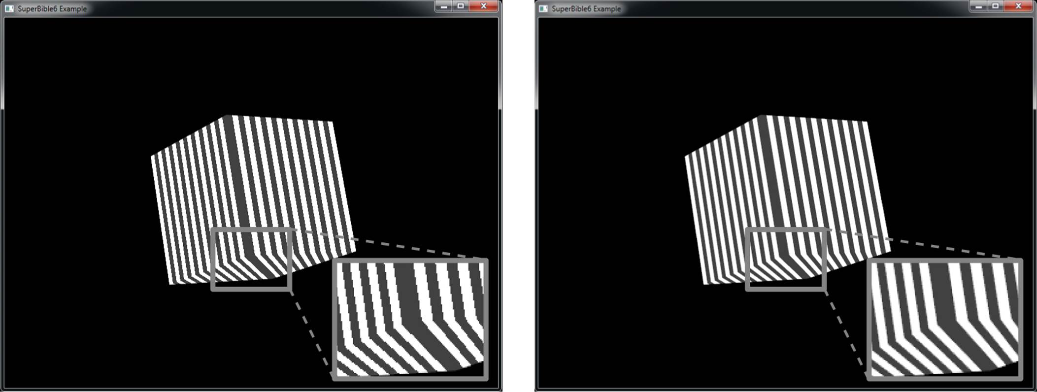
Figure 9.13: Antialiasing of high-frequency shader output

To produce the image on the right of Figure 9.13, we enabled sample-rate shading. In this mode, OpenGL will run your shader for each and every sample that a primitive hits. Be careful, though, as for 8-sample buffers, your shader will become 8 times more expensive! To enable sample rate shading, call

glEnable(GL_SAMPLE_SHADING);

and to disable sample rate shading, call

glDisable(GL_SAMPLE_SHADING);

Once you have enabled sample shading, you also need to let OpenGL know what portion of the samples it should run your shader for. By default, simply enabling sample shading won’t do anything, and OpenGL will still run your shader once for each pixel. To tell OpenGL what fraction of the samples you want to shade independently, call glMinSampleShading(), whose prototype is

void glMinSampleShading(GLfloat value);

For example, if you want OpenGL to run your shader for at least half of the samples in the framebuffer, set the value parameter set to 0.5f. To uniquely shade every sample hit by the geometry, set value to 1.0f. As you can see from the right image of Figure 9.13, the jaggies on the interior of the cube have been eliminated. We set the minimum sampling fraction to 1.0 to create this image.

Centroid Sampling

The centroid storage qualifier controls where in a pixel OpenGL interpolates the inputs to the fragment shader to. It only applies to situations where you’re rendering into a multi-sampled framebuffer. You specify the centroid storage qualifier just like any other storage qualifier that is applied to an input or output variable. To create a varying that has the centroid storage qualifier, first, in the vertex, tessellation control, or geometry shader, declare the output with the centroid keyword:

centroid out vec2 tex_coord;

And then in the fragment shader, declare the same input with the centroid keyword:

centroid in vec2 tex_coord;

You can also apply the centroid qualifier to an interface block to cause all of the members of the block to be interpolated to the fragment’s centroid:

centroid out VS_OUT
{
vec2 tex_coord;
} vs_out;

Now tex_coord (or vs_out.tex_coord) is defined to use the centroid storage qualifier. If you have a single-sampled draw buffer, this makes no difference, and the inputs that reach the fragment shader are interpolated to the pixel’s center. Where centroid sampling becomes useful is when you are rendering to a multi-sampled draw buffer. According to the OpenGL Specification, when centroid sampling is not specified (the default), fragment shader varyings will be interpolated to “the pixel’s center, or anywhere within the pixel, or to one of the pixel’s samples” — which basically means anywhere within the pixel. When you’re in the middle of a large triangle, this doesn’t really matter. Where it becomes important is when you’re shading a pixel that lies right on the edge of the triangle — where an edge of the triangle cuts through the pixel. Figure 9.14 shows an example of how OpenGL might sample from a triangle.

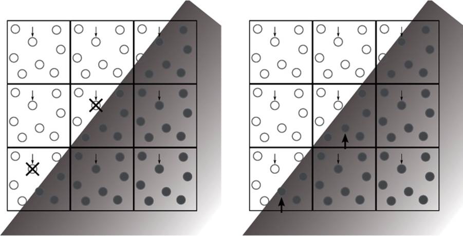
Figure 9.14: Partially covered multi-sampled pixels

Take a look at the left of Figure 9.14. It shows the edge of a triangle passing through several pixels. The solid dots represent samples that are covered by the triangle, and the clear dots represent those that are not. OpenGL has chosen to interpolate the fragment shader inputs to the sample closest to the pixel’s center. Those samples are indicated by a small downwards-pointing arrow.

For the pixels in the upper left, this is fine — they are entirely uncovered and the fragment shader will not run for those pixels. Likewise, the pixels in the lower right are fully covered. The fragment shader will run, but it doesn’t really matter which sample it runs for. The pixels along the edge of the triangle, however, present a problem. Because OpenGL has chosen the sample closest to the pixel center as its interpolation point, your fragment shader inputs could actually be interpolated to a point that lies outside the triangle! Those samples are marked with an X. Imagine what would happen if you used the input, say, to sample from a texture. If the texture was aligned such that its edge was supposed to match the edge of the triangle, the texture coordinates would lie outside the texture. At best, you would get a slightly incorrect image. At worst, it would produce noticeable artifacts.

If we declare our inputs with the centroid storage qualifier, the OpenGL Specification says that “the value must be interpolated to a point that lies in both the pixel and in the primitive being rendered, or to one of the pixel’s samples that falls within the primitive.” That means that OpenGL chooses, for each pixel, a sample that is certainly within the triangle to which to interpolate all varyings. You are safe to use the inputs to the fragment shader for any purpose, and you know that they are valid and have not been interpolated to a point outside the triangle.

Now look at the right side of Figure 9.14. OpenGL has still chosen to interpolate the fragment shader inputs to the samples closest to the pixel centers for fully covered pixels. However, for those pixels that are partially covered, it has instead chosen another sample that lies within the triangle (marked with larger arrows). This means that the inputs presented to the fragment shader are valid and refer to points that are inside the triangle. You can use them for sampling from a texture or use them in a function whose result is only defined within a certain range and know that you will get meaningful results.

You may be wondering whether using the centroid storage qualifier guarantees that you’re going to get valid results in your fragment shader and not using it may mean that the inputs are interpolated outside the primitive, why not turn on centroid sampling all the time? Well, there are some drawbacks to using centroid sampling.

The most significant is that OpenGL can provide the gradients (or differentials) of inputs to the fragment shader. Implementations may differ, but most use discrete differentials, taking deltas between the values of the same inputs from adjacent pixels. This works well when the inputs are interpolated to the same position within each pixel. In this case, it doesn’t matter which sample position is chosen; the samples will always be exactly one pixel apart. However, when centroid sampling is enabled for an input, the values for adjacent pixels may actually be interpolated to different positions within those pixels. That means that the samples are not exactly one pixel apart, and the discrete differentials presented to the fragment shader could be inaccurate. If accurate gradients are required in the fragment shader, it is probably best not to use centroid sampling. Don’t forget, the calculations that OpenGL performs during mipmapping depend on gradients of texture coordinates, and so using a centroid qualified input as the source of texture coordinates to a mipmapped texture could lead to inaccurate results.

Using Centroid Sampling to Perform Edge Detection

An interesting use case for centroid sampling is hardware-accelerated edge detection. You just learned that using the centroid storage qualifier ensures that your inputs are interpolated to a point that definitely lies within the primitive being rendered. To do this, OpenGL chooses a sample that it knows lies inside the triangle at which to evaluate those inputs, and that sample may be different from the one that it would have chosen if the pixel was fully covered or the one that it would choose if the centroid storage qualifier was not used. You can use this knowledge to your advantage.

To extract edge information from this, declare two inputs to your fragment shader, one with and one without the centroid storage qualifier, and assign the same value to each of them in the vertex shader. It doesn’t matter what the values are, so long as they are different for each vertex. The xand y components of the transformed vertex position are probably a good choice because you know that they will be different for each vertex of any triangle that is actually visible.

out vec2 maybe_outside;

gives us our non-centroid input that may be interpolated to a point outside the triangle, and

centroid out vec2 certainly_inside;

gives us our centroid sampled input that we know is inside the triangle. Inside the fragment shader, we can compare the values of the two varyings. If the pixel is entirely covered by the triangle, OpenGL uses the same value for both input. However, if the pixel is only partially covered by the triangle, OpenGL uses its normal choice of sample for maybe_outside and picks a sample that is certain to be inside the triangle for certainly_inside. This could be a different sample than was chosen for maybe_outside, and that means that the two inputs may have different values. Now you can compare them to determine that you are on the edge of a primitive:

bool may_be_on_edge = any(notEqual(maybe_outside,
certainly_inside));

This method is not foolproof. Even if a pixel is on the edge of a triangle, it is possible that it covers OpenGL’s original sample of choice, and therefore you still get the same values for maybe_outside and certainly_inside. However, this marks most edge pixels.

To use this information, you can write the value to a texture attached to the framebuffer and subsequently use that texture for further processing later. Another option is to draw only to the stencil buffer. Set your stencil reference to one, disable stencil testing, and set your stencil operation toGL_REPLACE. When you encounter an edge, let the fragment shader continue running. When you encounter a pixel that’s not on an edge, use the discard keyword in your shader to prevent the pixel from being written to the stencil buffer. The result is that your stencil buffer contains ones wherever there was an edge in the scene and zeros wherever there was no edge. Later, you can render a full-screen quad with an expensive fragment shader that only runs for pixels that represent the edges of geometry where a sample would have been chosen that was outside the triangle by enabling the stencil test, setting the stencil function to GL_EQUAL, and leaving the reference value at one. The shader could implement image processing operations at each pixel, for instance. Applying Gaussian blur using a convolution operation can smooth the edges of polygons in the scene, allowing the application to perform its own antialiasing.

Advanced Framebuffer Formats

Until now, you have been using either the window-system-supplied framebuffer (i.e., the default framebuffer), or you have rendered into textures using your own framebuffer. However, the textures you attached to the framebuffer have been of the format GL_RGBA8, which is an 8-bit unsigned normalized format. This means that it can only represent values between 0.0 and 1.0, in 256 steps. However, the output of your fragment shaders has been declared as vec4 — a vector of four floating-point elements. OpenGL can actually render into almost any format you can imagine, and framebuffer attachments can have one, two, three, or four components, can be floating-point or integer formats, can store negative numbers, and can be wider than 8 bits, providing much more definition.

In this section, we explore a few of the more advanced formats that can be used for framebuffer attachments and that allow you to capture more of the information that might be produced by your shaders.

Rendering with No Attachments

Just as you can attach multiple textures to a single framebuffer and render into all of them with a single shader, it’s also possible to create a framebuffer and not attach any textures to it at all. This may seem like a strange thing to do. You may ask where your data goes. Well, any outputs declared in the fragment shader have no effect, and data written to them will be discarded. However, fragment shaders can have a number of side effects besides writing to their outputs. For example, they can write into memory using the imageStore function, and they can also increment and decrement atomic counters using the atomicCounterIncrement and atomicCounterDecrement functions.

Normally, when a framebuffer object has one or more attachments, it derives its maximum width and height, layer count, and sample count from those attachments. These properties define the size to which the viewport will be clamped and so on. When a framebuffer object has no attachments, limits imposed by the amount of memory available for textures, for example, are removed. However, the framebuffer must derive this information from another source. Each framebuffer object therefore has a set of parameters that are used in place of those derived from its attachments when no attachments are present. To modify these parameters, call glFramebufferParameteri(), whose prototype is

void glFramebufferParameteri(GLenum target,
GLenum pname,
GLint param);

target specifies the target where the framebuffer object is bound, and may be GL_DRAW_FRAMEBUFFER, GL_READ_FRAMEBUFFER, or simply GL_FRAMEBUFFER. Again, If you specify GL_FRAMEBUFFER, then it is considered equivalent to GL_DRAW_FRAMEBUFFER, and the framebuffer object bound to theGL_DRAW_FRAMEBUFFER binding point will be modified. pname specifies which parameter you want to modify, and param is the value you want to change it to. pname can be one of the following:

• GL_FRAMEBUFFER_DEFAULT_WIDTH indicates that param contains the width of the framebuffer when it has no attachments.

• GL_FRAMEBUFFER_DEFAULT_HEIGHT indicates that param contains the height of the framebuffer when it has no attachments.

• GL_FRAMEBUFFER_DEFAULT_LAYERS indicates that param contains the layer count of the framebuffer when it has no attachments.

• GL_FRAMEBUFFER_DEFAULT_SAMPLES indicates that param contains the number of samples in the framebuffer when it has no attachments.

• GL_FRAMEBUFFER_DEFAULT_FIXED_SAMPLE_LOCATIONS indicates that param specifies whether the framebuffer uses the fixed default sample locations. If param is non-zero, then OpenGL’s default sample pattern will be used; otherwise, OpenGL might choose a more advanced arrangement of samples for you.

The maximum dimensions of a framebuffer without any attachments can be extremely large because no real storage for the attachments is required. Listing 9.23 demonstrates how to initialize a virtual framebuffer that is 10,000 pixels wide and 10,000 pixels high.

// Generate a framebuffer name and bind it.
Gluint fbo;

glGenFramebuffers(1, &fbo);
glBindFramebuffer(GL_FRAMEBUFFER, fbo);

// Set the default width and height to 10000
glFramebufferParameteri(GL_FRAMEBUFFER_DEFAULT_WIDTH, 10000);
glFramebufferParameteri(GL_FRAMEBUFFER_DEFAULT_HEIGHT, 10000);

Listing 9.23: A 100-megapixel virtual framebuffer

If you render with the framebuffer object created in Listing 9.23 bound, you will be able to use glViewport() to set the viewport size to 10,000 pixels wide and high. Although there are no attachments on the framebuffer, OpenGL will rasterize primitives as if the framebuffer were really that size, and your fragment shader will run. The values of the x and y components of gl_FragCoord variable will range from 0 to 9,999.

Floating-Point Framebuffers

One of the most useful framebuffer features is the ability to use attachments with floating-point formats. Although internally the OpenGL pipeline usually works with floating-point data, the sources (textures) and targets (framebuffer attachments) have often been fixed point and of significantly less precision. As a result, many portions of the pipeline used to clamp all values between 0 and 1 so they could be stored in a fixed-point format in the end.

The data type passed into your vertex shader is up to you but is typically declared as vec4, or a vector of four floats. Similarly, you decide what outputs your vertex shader should write when you declare variables as out in a vertex shader. These outputs are then interpolated across your geometry and passed into your fragment shader. You have complete control of the type of data you decide to use for color throughout the whole pipeline, although it’s most common to just use floats. You now have complete control over how and in what format your data is in as it travels from vertex arrays all the way to the final output.

Now instead of 256 values, you can color and shade using values from 1.18 × 10^–³⁸ all the way to 3.4 × 10³⁸! You may wonder what happens if you are drawing to a window or monitor that only supports 8 bits per color. Unfortunately, the output is clamped to the range of 0 to 1 and then mapped to a fixed-point value. That’s no fun! Until someone invents monitors or displays⁶ that can understand and display floating-point data, you are still limited by the final output device.

6. Some very high-end monitors are available today that can interpret 10 or even 12 bits of data in each channel. However, they’re often prohibitively expensive, and there aren’t any displays that accept floating-point data outside of the lab.

That doesn’t mean floating-point rendering isn’t useful though. Quite the contrary! You can still render to textures in full floating-point precision. Not only that, but you have complete control over how floating-point data gets mapped to a fixed output format. This can have a huge impact on the final result and is commonly referred to high dynamic range, or HDR.

Using Floating-Point Formats

Upgrading your applications to use floating-point buffers is easier than you may think. In fact, you don’t even have to call any new functions. Instead, there are two new tokens you can use when creating buffers, GL_RGBA16F and GL_RGBA32F. These can be used when creating storage for textures:

glTexStorage2D(GL_TEXTURE_2D, 1, GL_RGBA16F, width, height);
glTexStorage2D(GL_TEXTURE_2D, 1, GL_RGBA32F, width, height);

In addition to the more traditional RGBA formats, Table 9.8 lists other formats allowed for creating floating-point textures. Having so many floating-point formats available allows applications to use the format that most suits the data that they will produce directly.

Table 9.8. Floating-Point Texture Formats

As you can see, there are 16- and 32-bit floating-point formats with one, two, three, and four channels. There is also a special format, GL_R11F_G11F_B10F, that contains two 11-bit floating-point components and one 10-bit component, packed together in a single 32-bit word. These are special, unsigned floating-point formats⁷ with a 5-bit exponent and a 6-bit mantissa in the 11-bit components, and a 5-bit exponent and mantissa for the 10-bit component.

7. Floating-point data is almost always signed, but it is possible to sacrifice the sign bit if only positive numbers will ever be stored.

In addition to the formats shown in Table 9.8, you can also create textures that have the GL_DEPTH_COMPONENT32F or GL_DEPTH_COMPONENT32F_STENCIL8 formats. The first is used to store depth information and such textures can be used as depth attachments on a framebuffer. The second represents both depth and stencil information stored in a single texture. This can be used for both the depth attachment and the stencil attachment of a framebuffer object.

High Dynamic Range

Many modern game applications use floating-point rendering to generate all of the great eye candy we now expect. The level of realism possible when generating lighting effects such as light bloom, lens flare, light reflections, light refractions, crepuscular rays, and the effects of participating media such as dust or clouds are often not possible without floating-point buffers. High dynamic range (HDR) rendering into floating-point buffers can make the bright areas of a scene really bright, keep shadow areas very dark, and still allow you to see detail in both. After all, the human eye has an incredible ability to perceive very high contrast levels well beyond the capabilities of today’s displays.

Instead of drawing a complex scene with a lot of geometry and lighting in our sample programs to show how effective HDR can be, we use images already generated in HDR for simplicity. The first sample program, hdr_imaging, loads HDR (floating-point) images from .KTX files that store the original, floating-point data in its raw form. These images are generated by taking a series of aligned images of a scene with different exposures and then combining them together to produce an HDR result.

The low exposures capture detail in the bright areas of the scene while the high exposures capture detail in the dark areas of the scene. Figure 9.15 shows four views of a scene of a tree lit by bright decorative lights (these images are also shown in Color Plate 2). The top left image is rendered at a very low exposure and shows all of the detail of lights even though they are very bright. The top right image increases the exposure such that you start to see details in the ribbon. On the bottom left, the exposure is increased to the level that you can see details in the pine cones, and finally, on the bottom right, the exposure has increased such that the branches in the foreground become very clear. The four images show the incredible amount of detail and range that are stored in a single image.

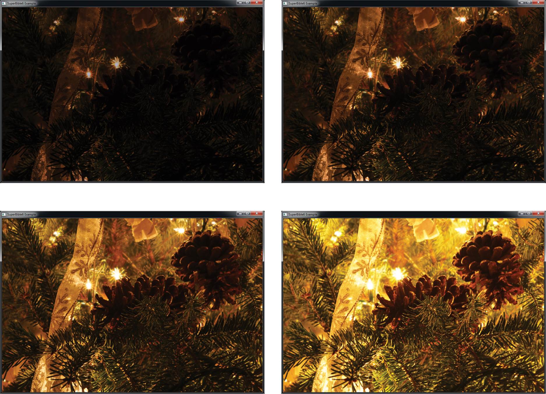
Figure 9.15: Different views of an HDR image

The only way possible to store so much detail in a single image is to use floating-point data. Any scene you render in OpenGL, especially if it has very bright or dark areas, can look more realistic when the true color output can be preserved instead of clamped between 0.0 and 1.0, and then divided into only 256 possible values.

Tone Mapping

Now that you’ve seen some of the benefits of using floating-point rendering, how do you use that data to generate a dynamic image that still has to be displayed using values from 0 to 255? Tone mapping is the action of mapping color data from one set of colors to another or from one color space to another. Because we can’t directly display floating-point data, it has to be tone mapped into a color space that can be displayed.

The first sample program, hdrtonemap, uses three approaches to map the high-definition output to the low-definition screen. The first method, enabled by pressing the 1 key, is a simple and naïve direct texturing of the floating-point image to the screen. The histogram of the HDR image inFigure 9.15 is shown in Figure 9.16. From the graph, it is clear while that most of the image data has values between 0.0 and 1.0, many of the important highlights are well beyond 1.0. In fact, the highest luminance level for this image is almost 5.5!

Figure 9.16: Histogram of levels for treelights.ktx

If we send this image directly to our regular 8-bit normalized back buffer, the result is that the image is clamped and all of the bright areas look white. Additionally, because the majority of the data is in the first quarter of the range, or between 0 and 63 when mapped directly to 8 bits, it all blends together to look black. Figure 9.17 shows the result; the bright areas such as the lamps are practically white, and the dark areas such as the pine cones the are nearly black.

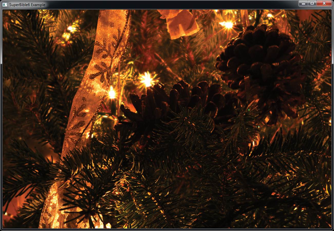
Figure 9.17: Naïve tone mapping by clamping

The second approach in the sample program is to vary the “exposure” of the image, similar to how a camera can vary exposure to the environment. Each exposure level provides a slightly different window into the texture data. Low exposures show the detail in the very bright sections of the scene; high exposures allow you to see detail in the dark areas but wash out the bright parts. This is similar to the images in Figure 9.15 with the low exposure on the upper left and the high exposure on the lower right. For our tone mapping pass, the hdrtonemap sample program reads from a floating-point texture and writes to the default framebuffer with an 8-bit back buffer. This allows the conversion from HDR to LDR (low dynamic range) to be on a pixel-by-pixel basis, which reduces artifacts that occur when a texel is interpolated between bright and dark areas. Once the LDR image has been generated, it can be displayed to the user. Listing 9.24 shows the simple exposure shader used in the example.

#version 430 core

layout (binding = 0) uniform sampler2D hdr_image;

uniform float exposure = 1.0;

out vec4 color;

void main(void)
{
vec4 c = texelFetch(hdr_image, ivec2(gl_FragCoord.xy), 0);
c.rgb = vec3(1.0) - exp(-c.rgb * exposure);
color = c;
}

Listing 9.24: Applying simple exposure coefficient to an HDR image

In the sample application, you can use the plus and minus keys on the numeric keypad to adjust the exposure. The range of exposures for this program goes from 0.01 to 20.0. Notice how the level of detail in different locations in the image changes with the exposure level. In fact, the images shown in Figure 9.15 were generated with this sample program by setting the exposure to different levels.

The last tone mapping shader used in the first sample program performs dynamic adjustments to the exposure level based on the relative brightness of different portions of the scene. First, the shader needs to know the relative luminance of the area near the current texel being tone mapped. The shader does this by sampling 25 texels centered around the current texel. All of the surrounding samples are then converted to luminance values, which are then weighted and added together. The sample program uses a non-linear function to convert the luminance to an exposure. In this example, the default curve is defined by the function

The shape of the curve is shown in Figure 9.18.

Figure 9.18: Transfer curve for adaptive tone mapping

The exposure is then used to convert the HDR texel to an LDR value using the same expression as in Listing 9.24. Listing 9.25 shows the adaptive HDR shader.

#version 430 core
// hdr_adaptive.fs
//
//

in vec2 vTex;

layout (binding = 0) uniform sampler2D hdr_image;

out vec4 oColor;

void main(void)
{
int i;
float lum[25];
vec2 tex_scale = vec2(1.0) / textureSize(hdr_image, 0);

for (i = 0; i < 25; i++)
{
vec2 tc = (2.0 * gl_FragCoord.xy +
3.5 * vec2(i % 5 - 2, i / 5 - 2));
vec3 col = texture(hdr_image, tc * tex_scale).rgb;
lum[i] = dot(col, vec3(0.3, 0.59, 0.11));
}

// Calculate weighted color of region
vec3 vColor = texelFetch(hdr_image,
2 * ivec2(gl_FragCoord.xy), 0).rgb;

float kernelLuminance = (
(1.0 * (lum[0] + lum[4] + lum[20] + lum[24])) +
(4.0 * (lum[1] + lum[3] + lum[5] + lum[9] +
lum[15] + lum[19] + lum[21] + lum[23])) +
(7.0 * (lum[2] + lum[10] + lum[14] + lum[22])) +
(16.0 * (lum[6] + lum[8] + lum[16] + lum[18])) +
(26.0 * (lum[7] + lum[11] + lum[13] + lum[17])) +
(41.0 * lum[12])
) / 273.0;

// Compute the corresponding exposure
float exposure = sqrt(8.0 / (kernelLuminance + 0.25));

// Apply the exposure to this texel
oColor.rgb = 1.0 - exp2(-vColor * exposure);
oColor.a = 1.0f;
}

Listing 9.25: Adaptive HDR to LDR conversion fragment shader

When using one exposure for an image, you can adjust for the best results by taking the range for the whole and using an average. Considerable detail is still lost with this approach in the bright and dim areas. The non-linear transfer function used with the adaptive fragment shader brings out the detail in both the bright and dim areas of the image; take a look at Figure 9.19. The transfer function uses a logarithmic-like scale to map luminance values to exposure levels. You can change this function to increase or decrease the range of exposures used and the resulting amount of detail in different dynamic ranges.

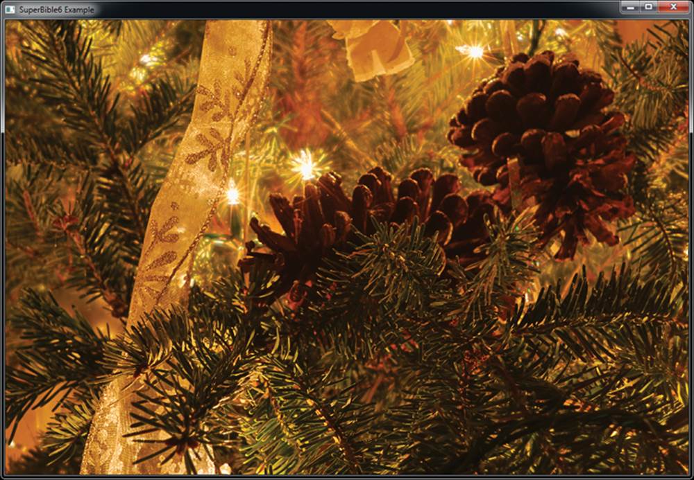
Figure 9.19: Result of adaptive tone mapping program

Figure 9.19 is also shown in Color Plate 3. Great, so now you know how to image process an HDR file, but what good is that in a typical OpenGL program? Lots! The HDR image is only a stand-in for any lit OpenGL scene. Many OpenGL games and applications now render HDR scenes and other content to floating-point framebuffer attachments and then display the result by doing a final pass using a technique such as one discussed above. You can use the same methods you just learned to render in HDR, generating much more realistic lighting environments and showing the dynamic range and detail of each frame.

Making Your Scene Bloom

One of the effects that works very well with high dynamic range images is the bloom effect. Have you ever noticed how the sun or a bright light can sometimes engulf tree branches or other objects between you and the light source? That’s called light bloom. Figure 9.20 shows how light bloom can affect an indoor scene.

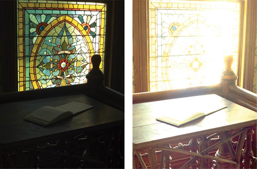
Figure 9.20: The effect of light bloom on an image

Notice how you can see all the detail in the lower exposure of the left side of Figure 9.20. The right side is a much higher exposure, and the grid in the stained glass is covered by the light bloom. Even the wooden post on the bottom right looks smaller as it gets covered by bloom. By adding bloom to a scene you can enhance the sense of brightness in certain areas. We can simulate this bloom effect caused by bright light sources. Although you could also perform this effect using 8-bit precision buffers, it’s much more effective when used with floating-point buffers on a high dynamic range scene.

The first step is to draw your scene in with high dynamic range. For the hdrbloom sample program, an framebuffer is set up with two floating-point textures bound as color attachments. The scene is rendered as normal to the first bound texture. But the second bound texture gets only the bright areas of the field. The hdrbloom sample program fills both textures in one pass from one shader (see Listing 9.26). The output color is computed as normal and sent to the color0 output. Then, the luminance (brightness) value of the color is calculated and used to threshold the data. Only the brightest data is used to generate the bloom effect and is written to the second output, color1. The threshold levels used are adjustable via a pair of uniforms, bloom_thresh_min and bloom_thresh_max. To filter for the bright areas, we use the smoothstep function to smoothly force any fragments whose brightness is less than bloom_thresh_min to zero, and any fragments whose brightness is greater than bloom_thresh_max to four times the original color output.

#version 430 core

layout (location = 0) out vec4 color0;
layout (location = 1) out vec4 color1;

in VS_OUT
{
vec3 N;
vec3 L;
vec3 V;
flat int material_index;
} fs_in;

// Material properties
uniform float bloom_thresh_min = 0.8;
uniform float bloom_thresh_max = 1.2;

struct material_t
{
vec3 diffuse_color;
vec3 specular_color;
float specular_power;
vec3 ambient_color;
};

layout (binding = 1, std140) uniform MATERIAL_BLOCK
{
material_t material[32];
} materials;

void main(void)
{
// Normalize the incoming N, L, and V vectors
vec3 N = normalize(fs_in.N);
vec3 L = normalize(fs_in.L);
vec3 V = normalize(fs_in.V);

// Calculate R locally
vec3 R = reflect(-L, N);

material_t m = materials.material[fs_in.material_index];

// Compute the diffuse, and specular components for each fragment
vec3 diffuse = max(dot(N, L), 0.0) * m.diffuse_color;
vec3 specular = pow(max(dot(R, V), 0.0), m.specular_power) * m.specular_color;
vec3 ambient = m.ambient_color;

// Add ambient, diffuse, and specular to find final color
vec3 color = ambient + diffuse + specular;

// Write final color to the framebuffer
color0 = vec4(color, 1.0);

// Calculate luminance
float Y = dot(color, vec3(0.299, 0.587, 0.144));

// Threshold color based on its luminance, and write it to
// the second output
color = color * 4.0 * smoothstep(bloom_thresh_min, bloom_thresh_max, Y);
color1 = vec4(color, 1.0);
}

Listing 9.26: Bloom fragment shader; output bright data to a separate buffer

After the first shader has run, we obtain the two images shown in Figure 9.21. The scene we rendered is just a large collection of spheres with varying material properties. Some of them are configured to actually emit light as they have properties that will produce values in the framebuffer greater than one no matter what the lighting effects are. The image on the left is the scene rendered with no bloom. You will notice that it is sharp in all areas, regardless of brightness. The image on the right is the thresholded version of the image, which will be used as input to the bloom filters.

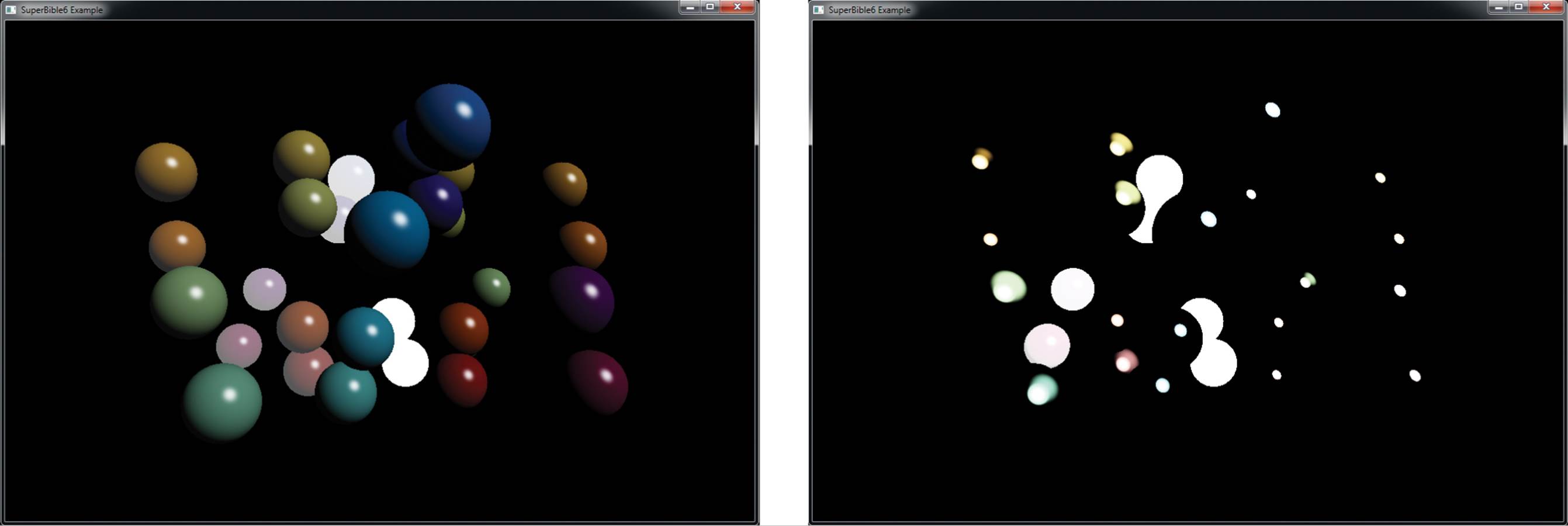
Figure 9.21: Original and thresholded output for bloom example

Now, after the scene has been rendered, there is still some work to do to finish the bright pass. The bright data must be blurred for the bloom effect to work. To implement this, we use a separable Gaussian filter. A separable filter is a filter that can be separated into two passes — generally one in the horizontal axis and one in the vertical. In this example, we use 25 taps in

each dimension, sampling from the 25 samples around the center of the filter and multiplying each texel by a fixed set of weights. To apply a separable filter, we make two passes. In the first pass, we filter in the horizontal dimension. However, you may notice that we use gl_FragCoord.yx to determine the center of our filter kernel. This means that we will transpose the image during filtering. However, on the second pass, we apply the same filter again. This means that filtering in the horizontal axis is equivalent to filtering in the vertical axis of the original image, and the output image is transposed again, returning it to its original orientation. In effect, we have performed a 2D Gaussian filter with a diameter of 25 samples and a total sample count of 625. The shader that implements this is shown in Listing 9.27.

#version 430 core

layout (binding = 0) uniform sampler2D hdr_image;

out vec4 color;

const float weights[] = float[](0.0024499299678342,
0.0043538453346397,
0.0073599963704157,
0.0118349786570722,
0.0181026699707781,
0.0263392293891488,
0.0364543006660986,
0.0479932050577658,
0.0601029809166942,
0.0715974486241365,
0.0811305381519717,
0.0874493212267511,
0.0896631113333857,
0.0874493212267511,
0.0811305381519717,
0.0715974486241365,
0.0601029809166942,
0.0479932050577658,
0.0364543006660986,
0.0263392293891488,
0.0181026699707781,
0.0118349786570722,
0.0073599963704157,
0.0043538453346397,
0.0024499299678342);
void main(void)
{
vec4 c = vec4(0.0);
ivec2 P = ivec2(gl_FragCoord.yx) - ivec2(0, weights.length() >> 1);
int i;

for (i = 0; i < weights.length(); i++)
{
c += texelFetch(hdr_image, P + ivec2(0, i), 0) * weights[i];
}

color = c;
}

Listing 9.27: Blur fragment shader

The result of applying blur to the thresholded image shown on the right of Figure 9.21 is shown in Figure 9.22.

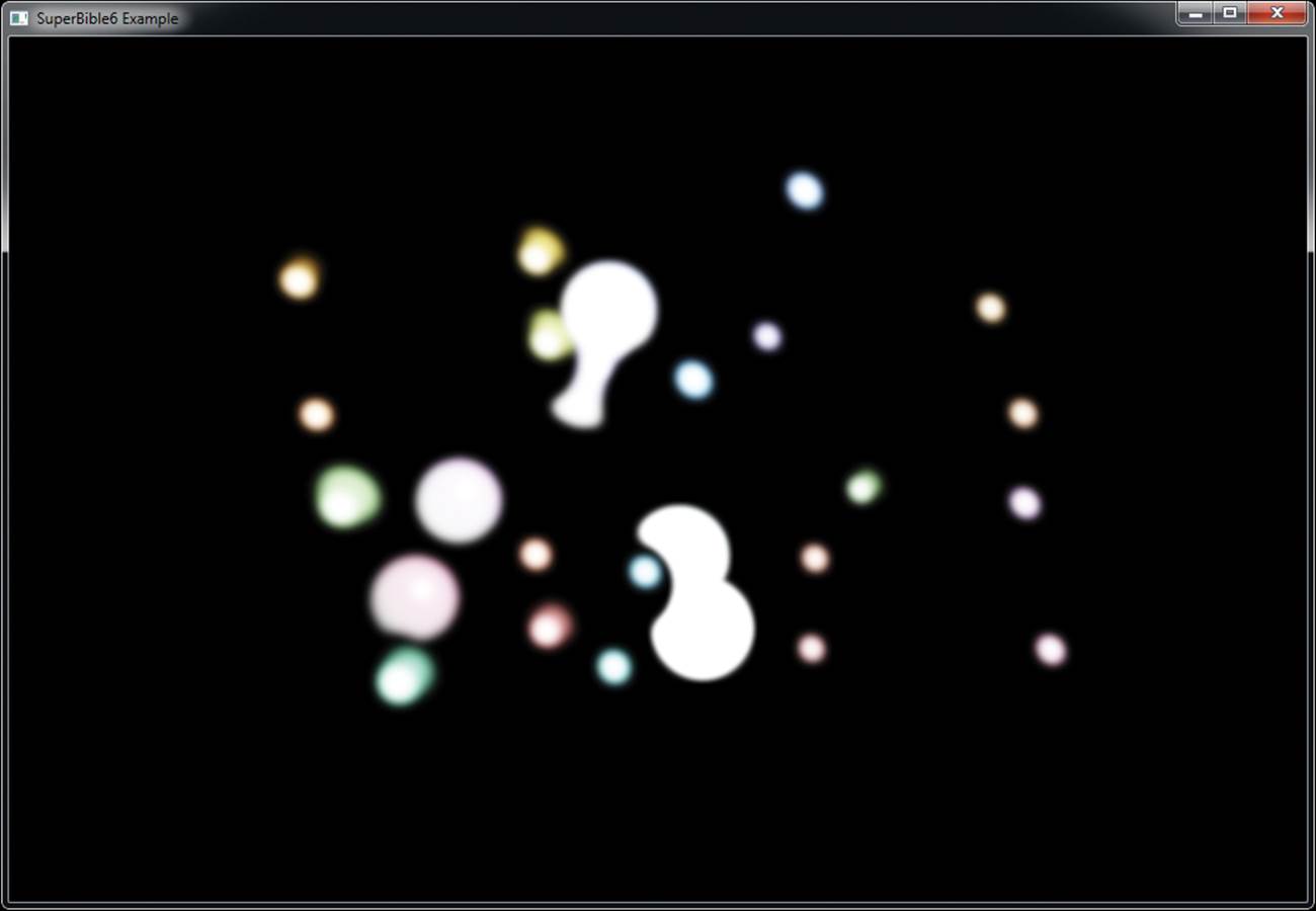
Figure 9.22: Blurred thresholded bloom colors

After the blurring passes are complete, the blur results are combined with the full color texture of the scene to produce the final results. In Listing 9.28 you can see how the final shader samples from two textures: the original full color texture and the blurred version of the bright pass. The original colors and the blurred results are added together to form the bloom effect, which is multiplied by a user-controlled uniform. The final high dynamic range color result is then put through exposure calculations, which you should be familiar with from the last sample program.

The exposure shader shown in Listing 9.28 is used to draw a screen-sized textured quad to the window. That’s it! Dial up and down the bloom effect to your heart’s content. Figure 9.23 shows the hdrbloom sample program with a high bloom level.

#version 430 core

layout (binding = 0) uniform sampler2D hdr_image;
layout (binding = 1) uniform sampler2D bloom_image;

uniform float exposure = 0.9;
uniform float bloom_factor = 1.0;
uniform float scene_factor = 1.0;

out vec4 color;

void main(void)
{
vec4 c = vec4(0.0);

c += texelFetch(hdr_image, ivec2(gl_FragCoord.xy), 0) * scene_factor;
c += texelFetch(bloom_image, ivec2(gl_FragCoord.xy), 0) * bloom_factor;

c.rgb = vec3(1.0) - exp(-c.rgb * exposure);
color = c;
}

Listing 9.28: Adding bloom effect to scene

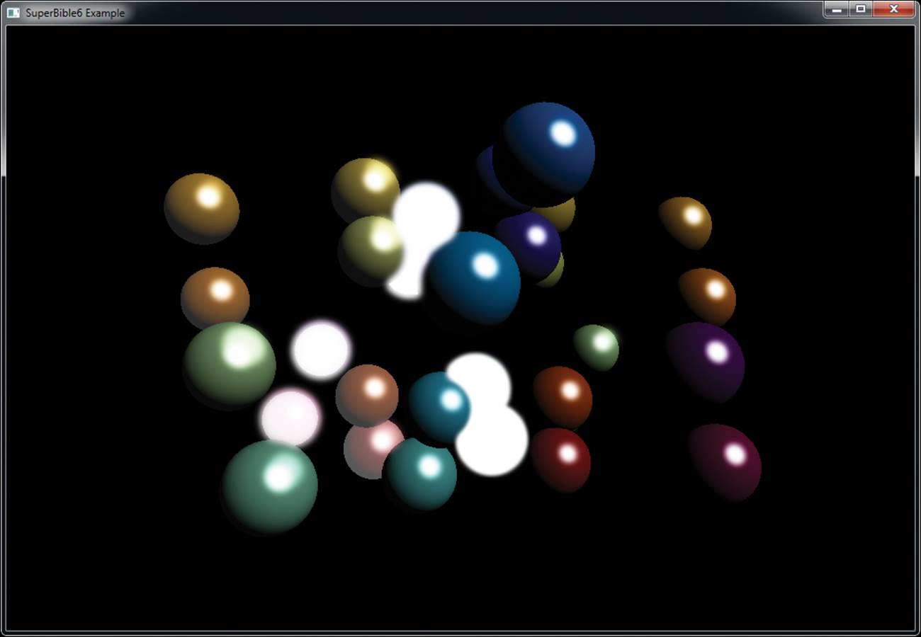
Figure 9.23: Result of the bloom program

A comparison of the output of this program with and without bloom is shown in Color Plate 4.

Integer Framebuffers

By default, the window system will provide your application with a fixed-point back buffer. When you declare a floating-point output from your fragment shader (such as a vec4), OpenGL will convert the data you write into it into a fixed-point representation suitable for storage in that framebuffer. In the previous section we covered floating-point framebuffer attachments, which provide the capability of storing an arbitrary floating-point value in the framebuffer. It’s also possible to create an integer framebuffer attachment by creating a texture with an integer internal format and attaching it to a framebuffer object. When you do this, it’s possible to use an output with an integer component type such as ivec4 or uvec4. With an integer framebuffer attachment, the bit pattern contained in your output variables will be written verbatim into the texture. You don’t need to worry about denormals, negative zero, infinities, or any other special bit patterns that might be a concern with floating-point buffers.

To create an integer framebuffer attachment, simply create a texture with an internal format made up an integer components and attach it to a framebuffer object. Internal formats that are made up of integers generally end in I or UI — for example, GL_RGBA32UI represents a format made up of four unsigned 32-bit integers per texel, and GL_R16I is a format made up of a single signed 16-bit component per texel. Code to create a framebuffer attachment with an internal format of GL_RGBA32UI is shown in Listing 9.29.

// Variables for the texture and FBO
GLuint tex;
GLuint fbo;

// Create the texture object
glGenTextures(1, &tex);

// Bind it to the 2D target and allocate storage for it
glBindTexture(GL_TEXTURE_2D, tex);
glTexStorage2D(GL_TEXTURE_2D, 1, GL_RGBA32UI, 1024, 1024);

// Now create an FBO and attach the texure as normal
glGenFrambuffers(1, &fbo);
glBindFramebuffer(GL_FRAMEBUFFER, fbo);

glFramebufferTexture(GL_FRAMEBFUFFER,
GL_COLOR_ATTACHMENT0,
tex,
0);

Listing 9.29: Creating integer framebuffer attachments

You can determine the component type of a framebuffer attachment by calling glGetFramebufferAttachmentParameteriv() with pname set to GL_FRAMEBUFFER_ATTACHMENT_COMPONENT_TYPE. The value returned in params will be GL_FLOAT, GL_INT, GL_UNSIGNED_INT, GL_SIGNED_NORMALIZED, orGL_UNSIGNED_NORMALIZED depending on the internal format of the color attachments. There is no requirement that the attachments to a framebuffer object all be of the same type. This means that you can have a combination of attachments, some of which are floating point or fixed point and others that are integer formats.

When you render to an integer framebuffer attachment, the output declared in your fragment shader should match that of the attachment in component type. For example, if your framebuffer attachment is an unsigned integer format such as GL_RGBA32UI, then your shader’s output variable corresponding to that color attachment should be an unsigned integer format such as unsigned int, uvec2, uvec3, or uvec4. Likewise, for signed integer formats, your output should be int, ivec2, ivec3, or ivec4. Although the component formats should match, there is no requirement that the number of components match.

If the component width of the framebuffer attachment is less than 32 bits, then the additional most significant bits will be thrown away when you render to it. You can even write floating-point data directly into an integer color buffer by using the GLSL functions floatBitsToInt (orfloatBitsToUint) or the packing functions such as packUnorm2x16.

While it may seem that integer framebuffer attachments offer some level of flexibility over traditional fixed- or floating-point framebuffers — especially in light of being able to write floating-point data into them,— there are some trade-offs that must be considered. The first and most glaring is that blending is not available for integer framebuffers. The other is that having an integer internal format means that the resulting texture into which you rendered your image cannot be filtered.

The sRGB Color Space

Eons ago, computer users had large, clunky monitors made from glass vacuum bottles called cathode ray tubes (CRTs). These devices worked by shooting electrons at a fluorescent screen to make it glow. Unfortunately, the amount of light emitted by the screen was not linear in the voltage used to drive it. In fact, the relationship between light output and driving voltage was highly nonlinear. The amount of light output was a power function of the form

To make matters worse, γ didn’t always take the same value. For NTSC systems (the television standard used in North America, much of South America, and parts of Asia), γ was about 2.2. However, with SECAM and PAL systems (the standards used in Europe, Australia, Africa, and other parts of Asia) used a γ value of 2.8. That means that if you put a voltage of half the maximum into a CRT-based display, you’d get a little less than one quarter of the maximum possible light output!

To compensate for this, in computer graphics we apply gamma correction (after the γ term in the power function) by raising linear values by a small power, scaling the result, and offsetting it. The resulting color space is known as sRGB, and the pseudo-code to translate from a linear value to an sRGB value is as follows:

if (cl >= 1.0)
{
cs = 1.0;
}
else if (cl <= 0.0)
{
cs = 0.0;
}
else if (cl < 0.0031308)
{
cs = 12.92 * cl;
}
else
{
cs = 1.055 * pow(cl, 0.41666) - 0.055;
}

Further, to go from sRGB to linear color space, we apply the transformation illustrated by the following pseudo-code:

if (cs >= 1.0)
{
cl = 1.0;
}
else if (cs <= 0.0)
{
cl = 0.0;
}
else if (cs <= 0.04045)
{
cl = cs / 12.92;
}
else
{
cl = pow((cs + 0.0555) / 1.055), 2.4)
}

In both cases, cs is the sRGB color space value, and cl is the linear value. Notice that the transformation has a short linear section and a small bias. In practice, this is so close to raising our linear color values to the powers 2.2 (for sRGB to linear) and 0.454545, which is (for linear to sRGB), that some implementations will do this. Figure 9.24 shows the transfer functions of linear to sRGB and sRGB back to linear on the left, and a pair of simple power curves using the powers 2.2 and 0.45454 on the right. You should notice that the shapes of these curves are so close as to be almost indistinguishable.

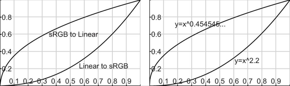
Figure 9.24: Gamma curves for sRGB and simple powers

To use the sRGB color space in OpenGL, we create textures with SRGB internal formats. For example, the GL_SRGB8_ALPHA8 represents the red, green, and blue components with an sRGB gamma ramp (the alpha component) is linear. We can load data into the texture as usual. When you read from an sRGB texture in your shader, the sRGB format is converted to RGB when the texture is sampled but before it is filtered. That is, when bilinear filtering is turned on, the incoming texels are converted from sRGB to linear, and then the linear samples are blended together to form the final value returned to the shader. Also, only the RGB components are converted separately, and the alpha is left as is.

Framebuffers also support storage formats that are sRGB; specifically, the format GL_SRGB8_ALPHA8 must be supported. That means you can attach textures that have an internal sRGB format to a framebuffer object and then render to it. Because we just talked about how sRGB formats are not linear, you probably don’t want your writes to sRGB framebuffer attachments to be linear either; that would defeat the whole purpose! The good news is OpenGL can convert the linear color values your shader outputs into sRGB values automatically. However, this isn’t performed by default. To turn this feature on, you need to call glEnable() with the GL_FRAMEBUFFER_SRGB token. Remember, this only works for color attachments that contain an sRGB surface. You can call glGetFramebufferAttachmentParameteriv() with the value GL_FRAMEBUFFER_ATTACHMENT_COLOR_ENCODING to find out if the attached surface is sRGB. sRGB surfaces return GL_SRGB, while other surfaces return GL_LINEAR.

Point Sprites

The term point sprites is usually used to refer to textured points. OpenGL represents each point by a single vertex, and so there is no opportunity to specify texture coordinates that can be interpolated as there is with the other primitive types. To get around this, OpenGL will generate an interpolated texture coordinate for you with which you can do anything you like. With point sprites, you can place a 2D textured image anywhere on-screen by drawing a single 3D point.

One of the most common applications of point sprites is for particle systems. A large number of particles moving on-screen can be represented as points to produce a number of visual effects. However, representing these points as small overlapped 2D images can produce dramatic streaming animated filaments. For example, Figure 9.25 shows a well-known screen saver on the Macintosh powered by just such a particle effect.

Figure 9.25: A particle effect in the flurry screen saver

Without point sprites, achieving this type of effect would be a matter of drawing a large number of textured quads (or triangle fans) on-screen. This could be accomplished either by performing a costly rotation to each individual face to make sure that it faced the camera, or by drawing all particles in a 2D orthographic projection. Point sprites allow you to render a perfectly aligned textured 2D square by sending down a single 3D vertex. At one-quarter the bandwidth of sending down four vertices for a quad and no matrix math to keep the 3D quad aligned with the camera, point sprites are a potent and efficient feature of OpenGL.

Texturing Points

Point sprites are easy to use. On the application side, the only thing you have to do is simply bind a 2D texture and read from it in your fragment shader using a built-in variable called gl_PointCoord, which is a two-component vector that interpolates the texture coordinates across the point.Listing 9.30 shows the fragment shader for the PointSprites example program.

#version 430 core

out vec4 vFragColor;

in vec4 vStarColor;

layout (binding = 0) uniform sampler2D starImage;

void main(void)
{
vFragColor = texture(starImage, gl_PointCoord) * vStarColor;
}

Listing 9.30: Texturing a point sprite in the fragment shader

Again, for a point sprite, you do not need to send down texture coordinates as an attribute as OpenGL will produce gl_PointCoord automatically. Since a point is a single vertex, you wouldn’t have the ability to interpolate across the points surface any other way. Of course, there is nothing preventing you from providing a texture coordinate anyway or deriving your own customized interpolation scheme.

Rendering a Star Field

Let’s now take a look at an example program that makes use of the point sprite features discussed so far. The starfield example program creates an animated star field that appears as if you were flying forward through it. This is accomplished by placing random points out in front of your field of view and then passing a time value into the vertex shader as a uniform. This time value is used to move the point positions so that over time they move closer to you and then recycle when they get to the near clipping plane to the back of the frustum. In addition, we scale the size of the stars so that they start off very small but get larger as they get closer to your point of view. The result is a nice realistic effect... all we need is some planetarium or space movie music!

Figure 9.26 shows our star texture map that is applied to the points. It is simply a .KTX file that we load in the same manner we loaded any other 2D texture so far. Points can also be mipmapped, and because they can range from very small to very large, it’s probably a good idea to do so.

Figure 9.26: The star texture map

We are not going to cover all of the details of setting up the star field effect, as it’s pretty routine and you can check the source yourself if you want to see how we pick random numbers. Of more importance is the actual rendering of code in the RenderScene function:

void render(double currentTime)
{
static const GLfloat black[] = { 0.0f, 0.0f, 0.0f, 0.0f };
static const GLfloat one[] = { 1.0f };
float t = (float)currentTime;
float aspect = (float)info.windowWidth /
(float)info.windowHeight;
vmath::mat4 proj_matrix = vmath::perspective(50.0f,
aspect,
0.1f,
1000.0f);
t *= 0.1f;
t -= floor(t);

glViewport(0, 0, info.windowWidth, info.windowHeight);
glClearBufferfv(GL_COLOR, 0, black);
glClearBufferfv(GL_DEPTH, 0, one);

glEnable(GL_PROGRAM_POINT_SIZE);
glUseProgram(render_prog);

glUniform1f(uniforms.time, t);
glUniformMatrix4fv(uniforms.proj_matrix, 1, GL_FALSE, proj_matrix);

glEnable(GL_BLEND);
glBlendFunc(GL_ONE, GL_ONE);

glBindVertexArray(star_vao);

glDrawArrays(GL_POINTS, 0, NUM_STARS);
}

We are going to use additive blending to blend our stars with the background. Because the dark area of our texture is black (zero in color space), we can get away with just adding the colors together as we draw. Transparency with alpha would require that we depth-sort our stars, and that is an expense we certainly can do without. After turning on point size program mode, we bind our shader and set up the uniforms. Of interest here is that we use the current time, which drives what will end up being the z position of our stars, that recycles so that it just counts smoothly from 0 to 1.Listing 9.31 provides the source code to the vertex shader.

#version 430 core

layout (location = 0) in vec4 position;
layout (location = 1) in vec4 color;

uniform float time;
uniform mat4 proj_matrix;

flat out vec4 starColor;

void main(void)
{
vec4 newVertex = position;

newVertex.z += time;
newVertex.z = fract(newVertex.z);

float size = (20.0 * newVertex.z * newVertex.z);

starColor = smoothstep(1.0, 7.0, size) * color;

newVertex.z = (999.9 * newVertex.z) - 1000.0;
gl_Position = proj_matrix * newVertex;
gl_PointSize = size;
}

Listing 9.31: Vertex shader for the star field effect

The vertex z component is offset by the time uniform. This is what causes the animation where the stars move closer to you. We only use the fractional part of this sum so that their position loops back to the far clipping plane as they get closer to the viewer. At this point in the shader, vertices with a z coordinate of 0.0 are at the far plane and vertices with a z coordinate of 1.0 are at the near plane. We can use the square of the vertex’s z coordinate to make the stars grow ever larger as they get nearer and set the final size in the gl_PointSize variable. If the star sizes are too small, you will get flickering sometimes, so we dim the color progressively using the smoothstep function so that any points with a size less than 1.0 will be black, fading to full intensity as they reach 7 pixels in size. This way, they fade into view instead of just popping up near the far clipping plane. The star color is passed to the fragment shader shown in Listing 9.32, which simply fetches from our star texture and multiplies the result by the computed star color.

#version 430 core

layout (location = 0) out vec4 color;

uniform sampler2D tex_star;
flat in vec4 starColor;

void main(void)
{
color = starColor * texture(tex_star, gl_PointCoord);
}

Listing 9.32: Fragment shader for the star field effect

The final output of the starfield program is shown in Figure 9.27.

Figure 9.27: Flying through space with point sprites

Point Parameters

A couple of features of point sprites (and points in general, actually) can be fine-tuned with the function glPointParameteri(). Figure 9.28 shows the two possible locations of the origin (0,0) of the texture applied to a point sprite. On the left, we see the origin on the upper left of the point sprite, and on the right, we see the origin as the lower left.

Figure 9.28: Two potential orientations of textures on a point sprite

The default orientation for point sprites is GL_UPPER_LEFT. Setting the GL_POINT_SPRITE_COORD_ORIGIN parameter to GL_LOWER_LEFT places the origin of the texture coordinate system at the lower-left corner of the point:

glPointParameteri(GL_POINT_SPRITE_COORD_ORIGIN, GL_LOWER_LEFT);

When the point sprite origin is set to its default of GL_UPPER_LEFT, gl_PointCoord will be 0.0, 0.0 at the top left of the point as it is viewed on the screen. However, in OpenGL, window coordinates are considered to start at the lower left of the window (which is the convention that gl_FragCoordadheres to, for example). Therefore, to get our point sprite coordinates to follow the window coordinate conventions and align with gl_FragCoord, we set the point sprite coordinate origin to GL_LOWER_LEFT.

Shaped Points

There is more you can do with point sprites besides apply a texture using gl_PointCoord for texture coordinates. You can use gl_PointCoord to derive a number of things other than just texture coordinates. For example, you can make non-square points by using the discard keyword in your fragment shader to throw away fragments that lie outside your desired point shape. The following fragment shader code produces round points:

vec2 p = gl_PointCoord * 2.0 - vec2(1.0);
if (dot(p, p) > 1.0)
discard;

Or perhaps an interesting flower shape:

vec2 temp = gl_PointCoord * 2.0 - vec2(1.0);
if (dot(temp, temp) > sin(atan(temp.y, temp.x) * 5.0))
discard;

These are simple code snippets that allow arbitrary shaped points to be rendered. Figure 9.29 shows a few more examples of interesting shapes that can be generated this way.

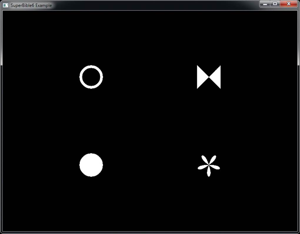
Figure 9.29: Analytically generated point sprite shapes

To create Figure 9.29, we used the fragment shader shown in Listing 9.33.

#version 430 core

layout (location = 0) out vec4 color;

flat in int shape;

void main(void)
{
color = vec4(1.0);
vec2 p = gl_PointCoord * 2.0 - vec2(1.0);

if (shape == 0)
{
// Simple disc shape
if (dot(p, p) > 1.0)
discard;
}
else if (shape == 1)
{
// Hollow circle
if (abs(0.8 - dot(p, p)) > 0.2)
discard;
}
else if (shape == 2)
{
// Flower shape
if (dot(p, p) > sin(atan(p.y, p.x) * 5.0))
discard;
}
else if (shape == 3)
{
// Bowtie
if (abs(p.x) < abs(p.y))
discard;
}
}

Listing 9.33: Fragment shader for generating shaped points

The advantage of calculating the shape of your points analytically in the fragment shader rather than using a texture is that the shapes are exact and stand up well to scaling and rotation, as you will see in the next section.

Rotating Points

Because points in OpenGL are rendered as axis-aligned squares, rotating the point sprite must be done by modifying the texture coordinates used to read the sprite’s texture or to analytically calculate its shape. To do this, you can simply create a 2D rotation matrix in the fragment shader and multiply it by gl_PointCoord to rotate it around the z axis. The angle of rotation could be passed from the vertex or geometry shader to the fragment shader as an interpolated variable. The value of the variable can, in turn, be calculated in the vertex or geometry shader or can be supplied through a vertex attribute. Listing 9.34 shows a slightly more complex point sprite fragment shader that allows the point to be rotated around its center.

This example allows you to generate rotated point sprites. However, the value of angle will not change from one fragment to another within the point sprite. That means that sin_theta and cos_theta will be constant, and the resulting rotation matrix constructed from them will also be the same for every fragment in the point. It is therefore much more efficient

#version 430

uniform sampler2D sprite_texture;

in float angle;

out vec4 color;

void main(void)
{
const float sin_theta = sin(angle);
const float cos_theta = cos(angle);
const mat2 rotation_matrix = mat2(cos_theta, sin_theta,
-sin_theta, cos_theta);
const vec2 pt = gl_PointCoord - vec2(0.5);
color = texture(sprite_texture, rotation_matrix * pt + vec2(0.5));
}

Listing 9.34: Naïve rotated point sprite fragment shader

to calculate sin_theta and cos_theta in the vertex shader and pass them as a pair of variables into the fragment shader rather than calculating them at every fragment. Here’s an updated vertex and fragment shader that allows you to draw rotated point sprites. First, the vertex shader is shown in Listing 9.35.

#version 430 core

uniform matrix mvp;

in vec4 position;
in float angle;

flat out float sin_theta;
flat out float cos_theta;

void main(void)
{
sin_theta = sin(angle);
cos_theta = cos(angle);

gl_Position = mvp * position;
}

Listing 9.35: Rotated point sprite vertex shader

And second, the fragment shader is shown in Listing 9.36.

#version 430 core

uniform sampler2D sprite_texture;

flat in float sin_theta;
flat in float cos_theta;

out vec4 color;

void main(void)
{
mat2 m = mat2(cos_theta, sin_theta,
-sin_theta, cos_theta);
const vec2 pt = gl_PointCoord - vec2(0.5);
color = texture(sprite_texture, rotation_matrix * pt + vec2(0.5));
}

Listing 9.36: Rotated point sprite fragment shader

As you can see, the potentially expensive sin and cos functions have been moved out of the fragment shader and into the vertex shader. If the point size is large, this pair of shaders performs much better than the earlier, brute force approach of calculating the rotation matrix in the fragment shader.

Remember that even though you are rotating the coordinates you derived from gl_PointCoord, the point itself is still square. If your texture or analytic shape spills outside the unit-diameter circle inside the point, you will need to make your point sprite larger and scale your texture coordinate down accordingly to get the shape to fit within the point under all angles of rotation. Of course, if your texture is essentially round, you don’t need to worry about this at all.

Getting at Your Image

Once everything’s rendered, your application will usually show the result to the user. The mechanism to do this is platform specific,⁸ and so the book’s application framework normally takes care of this for you. However, showing the result to the user might not always be what you want to do. There are many reasons why you might want to gain access to the rendered image directly from your application. For example, perhaps you want to print the image, save a screenshot, or even process it further with an offline process.

8. To read the details about how this works on several popular platforms, refer to Chapter 14.

Reading from a Framebuffer

To allow you to read pixel data from the framebuffer, OpenGL includes the glReadPixels() function, whose prototype is

void glReadPixels(GLint x,
GLint y,
GLsizei width,
GLsizei height,
GLenum format,
GLenum type,
GLvoid * data);

The glReadPixels() function will read the data from a region of the framebuffer currently bound to the GL_READ_FRAMEBUFFER target, or from the default framebuffer should no user-generated framebuffer object be bound, and write it into your application’s memory or into a buffer object. The xand y parameters specify the offset in window coordinates of the lower-left corner of the region, and width and height specify the width and height of the region to be read — remember, the origin of the window (which is at 0,0) is the lower-left corner. The format and type parameters tell OpenGL what format you want the data to be read back in. These parameters work similarly to the format and type parameters that you might pass to glTexSubImage2D(), for example. For instance, format might be GL_RED or GL_RGBA, and type might be GL_UNSIGNED_BYTE or GL_FLOAT. The resulting pixel data is written into the region specified by data.

If no buffer object is bound to the GL_PIXEL_PACK_BUFFER target, then data is interpreted as a raw pointer into your application’s memory. However, if a buffer is bound to the GL_PIXEL_PACK_BUFFER target, then data is treated as an offset into that buffer’s data store, and the image data is written there. If you want to get at that data, you can then map the buffer for reading by calling glMapBufferRange() with the GL_MAP_READ_BIT set and access the data. Otherwise, you could use the buffer for any other purpose.

To specify where the color data comes from, you can call glReadBuffer(), passing GL_BACK or GL_COLOR_ATTACHMENTi, where i indicates which color attachment you want to read from. The prototype of glReadBuffer() is

void glReadBuffer(GLenum mode);

If you are using the default framebuffer rather than your own framebuffer object, then mode should be GL_BACK. This is the default, so if you never use framebuffer objects in your application (or if you only ever read from the default framebuffer), you can get away without callingglReadBuffer() at all. However, since user-supplied framebuffer objects can have multiple attachments, you need to specify which attachment you want to read from, and so you must call glReadBuffer() if you are using your own framebuffer object.

When you call glReadPixels() with the format parameter set to GL_DEPTH_COMPONENT, the data read will come from the depth buffer. Likewise, if format is GL_STENCIL_INDEX, then the data comes from the stencil buffer. The special GL_DEPTH_STENCIL token allows you to read both the depth and stencil buffers at the same time. However, if you take this route, then the type parameter must be either GL_UNSIGNED_INT_24_8 or GL_FLOAT_32_UNSIGNED_INT_24_8_REV, which produces packed data that you would need to interpret to get at the depth and stencil information.

When OpenGL writes the data either into your application’s memory or into the buffer object bound to the GL_PIXEL_PACK_BUFFER target (if there is one bound), it writes it from left to right in order of ascending y coordinate, which, remember, has its origin at the bottom of the window and increases in an upward direction. By default, each row of the image starts at an offset from the previous, which is a multiple of four bytes. If the product of the width of the region to be read and the number of bytes per pixel is a multiple of four, then everything works out and the resulting data will be tightly packed. However, if things don’t add up, then you could be left with gaps in the output. You can change this by calling glPixelStorei(), whose prototype is

void glPixelStorei(GLenum pname,
GLint param);

When you pass GL_PACK_ALIGNMENT in pname, the value you pass in param is used to round the distance in bytes between each row of the image. You can pass 1 in param to set the rounding to a single byte, effectively disabling the rounding. The other values you can pass are 2, 4, and 8.

Taking a Screenshot

Listing 9.37 demonstrates how to take a screenshot of a running application and save it as a .TGA file, which is a relatively simple image file format that is easy to generate.

int row_size = ((info.windowWidth * 3 + 3) & ~3);
int data_size = row_size * info.windowHeight;
unsigned char * data = new unsigned char [data_size];

#pragma pack (push, 1)
struct
{
unsigned char identsize; // Size of following ID field
unsigned char cmaptype; // Color map type 0 = none
unsigned char imagetype; // Image type 2 = rgb
short cmapstart; // First entry in palette
short cmapsize; // Number of entries in palette
unsigned char cmapbpp; // Number of bits per palette entry
short xorigin; // X origin
short yorigin; // Y origin
short width; // Width in pixels
short height; // Height in pixels
unsigned char bpp; // Bits per pixel
unsigned char descriptor; // Descriptor bits
} tga_header;
#pragma pack (pop)

glReadPixels(0, 0, // Origin
info.windowWidth, info.windowHeight, // Size
GL_BGR, GL_UNSIGNED_BYTE, // Format, type
data); // Data

memset(&tga_header, 0, sizeof(tga_header));
tga_header.imagetype = 2;
tga_header.width = (short)info.windowWidth;
tga_header.height = (short)info.windowHeight;
tga_header.bpp = 24;

FILE * f_out = fopen("screenshot.tga", "wb");
fwrite(&tga_header, sizeof(tga_header), 1, f_out);
fwrite(data, data_size, 1, f_out);
fclose(f_out);

delete [] data;

Listing 9.37: Taking a screenshot with glReadPixels()

The .TGA file format simply consists of a header (which is defined by tga_header) followed by raw pixel data. The example of Listing 9.37 fills in the header and then immediately writes the raw data into the file immediately following it.

Copying Data between Framebuffers

Rendering to these off-screen framebuffers is fine and dandy, but ultimately you have to do something useful with the result. Traditionally, graphics APIs allowed an application to read pixel or buffer data back to system memory and also provided ways to draw it back to the screen. While these methods are functional, they required copying data from the GPU into CPU memory and then turning right around and copying it back. Very inefficient! We now have a way to quickly move pixel data from one spot to another using a blit command. Blit is a term that refers to direct, efficient bit-level data/memory copies. There are many theories of the origin of this term, but the most likely candidates are Bit-Level-Image-Transfer or Block-Transfer. Whatever the etymology of blit may be, the action is the same. Performing these copies is simple; the function looks like this:

void glBlitFramebuffer(GLint srcX0, Glint srcY0,
GLint srcX1, Glint srcY1,
GLint dstX0, Glint dstY0,
GLint dstX1, Glint dstY1,
GLbitfield mask, GLenum filter);

Even though this function has “blit” in the name, it does much more than a simple bitwise copy. In fact, it’s more like an automated texturing operation. The source of the copy is the read framebuffer’s read buffer specified by calling glReadBuffer(), and the area copied is the region defined by the rectangle with corners at (srcX0, srcY0) and (srcX1, srcY1). Likewise, the target of the copy is the current draw framebuffer’s draw buffer specified by calling glDrawBuffer(), and the area copied to is the region defined by the rectangle with corners at (dstX0, dstY0) and (dstX1, dstY1). Because the rectangles for the source and destination do not have to be of equal size, you can use this function to scale the pixels being copied. If you have set the read and draw buffers to the same FBO and have bound the same FBO to the GL_DRAW_FRAMEBUFFER and GL_READ_FRAMEBUFFERbindings, you can even copy data from one portion of a framebuffer to another (so long as you’re careful that the regions don’t overlap).

The mask argument can be any or all of GL_DEPTH_BUFFER_BIT, GL_STENCIL_BUFFER_BIT, or GL_COLOR_BUFFER_BIT. The filter can be either GL_LINEAR or GL_NEAREST, but it must be GL_NEAREST if you are copying depth or stencil data or color data with an integer format. These filters behave the same as they would for texturing. For our example, we are only copying non-integer color data and can use a linear filter.

GLint width = 800;
GLint height = 600;

GLenum fboBuffs[] = { GL_COLOR_ATTACHMENT0 };

glBindFramebuffer(GL_DRAW_FRAMEBUFFER, readFBO);
glBindFramebuffer(GL_READ_FRAMEBUFFER, drawFBO);

glDrawBuffers(1, fboBuffs);
glReadBuffer(GL_COLOR_ATTACHMENT0);
glBlitFramebuffer(0, 0, width, height,
(width *0.8), (height*0.8),
width, height,
GL_COLOR_BUFFER_BIT, GL_LINEAR );

Assume the width and height of the attachments of the FBO bound in the preceding code is 800 and 600. This code creates a copy of the whole of the first color attachment of readFBO, scales it down to 80% of the total size, and places it in the upper-left corner of the first color attachment ofdrawFBO.

Copying Data into a Texture

As you read in the last section, you can read data from the framebuffer into your application’s memory (or into a buffer object) by calling glReadPixels(), or from one framebuffer into another using glBlitFramebuffer(). If you intend to use this data as a texture, it may be more straightforward to simply copy the data directly from the framebuffer into the texture. The function to do this is glCopyTexSubImage2D(), and it is similar to glTexSubImage2D(), except that rather than taking source data from application memory or a buffer object, it takes its source data from the framebuffer. Its prototype is

void glCopyTexSubImage2D(GLenum target,
GLint level,
GLint xoffset,
GLint yoffset,
GLint x,
GLint y,
GLsizei width,
GLsizei height);

The target parameter is the texture target to which the destination texture is bound. For regular 2D textures, this will be GL_TEXTURE_2D, but you can also copy from the framebuffer into one of the faces of a cube map by specifying GL_TEXTURE_CUBE_MAP_POSITIVE_X,GL_TEXTURE_CUBE_MAP_NEGATIVE_X, GL_TEXTURE_CUBE_MAP_POSITIVE_Y, GL_TEXTURE_CUBE_MAP_NEGATIVE_Y, GL_TEXTURE_CUBE_MAP_POSITIVE_Z, or GL_TEXTURE_CUBE_MAP_NEGATIVE_Z. width and height represent the size of the region to be copied. x and y are the coordinates of the lower-left corner of the rectangle in the framebuffer, and xoffset and yoffset are the texel coordinates of the rectangle in the destination texture.

If your application renders directly into a texture (by attaching it to a framebuffer object), then this function might not be that useful to you. However if your application renders to the default framebuffer most of the time, you can use this function to move parts of the output into textures. If, on the other hand, you have data in a texture that you want to copy into another texture, you can achieve this by calling glCopyImageSubData(), which has a monstrous prototype:

void glCopyImageSubData(GLuint srcName,
GLenum srcTarget,
GLint srcLevel,
GLint srcX,
GLint srcY,
GLint srcZ,
GLuint dstName,
GLenum dstTarget,
GLint dstLevel,
GLint dstX,
GLint dstY,
GLint dstZ,
GLsizei srcWidth,
GLsizei srcHeight,
GLsizei srcDepth);

Unlike many of the other functions in OpenGL, this function operates directly on the texture objects you specify by name, rather than on objects bound to targets. srcName and srcTarget are the name and type of the source texture, and dstName and dstTarget are the name and type of the destination texture. You can pass pretty much any type of texture here, and so you have x, y, and z coordinates for the source and destination regions, and a width, height, and depth for each, too. srcX, srcY, and srcZ are the coordinates of the source region, and dstX, dstY, and dstZ are the coordinates of the destination region. The width, height, and depth of the region to copy is specified in srcWidth, srcHeight, and srcDepth.

If the textures you’re copying between don’t have a particular dimension (e.g., the z dimension for 2D textures doesn’t exist), you should set the corresponding coordinate to zero, and size to one.

If your textures have mipmaps, you can set the source and destination mipmap levels in srcLevel and dstLevel, respectively. Otherwise, set these to zero. Note that there is no destination width, height, or depth — the destination region is the same size as the source region, and no stretching or shrinking is possible. If you want to resize part of a texture and write the result into another texture, you’ll need to attach both to framebuffer objects and use glBlitFramebuffer().

Reading Back Texture Data

In addition to being able to read data from the framebuffer, you can also read image data from a texture by binding it to the appropriate texture target and then calling

void glGetTexImage(GLenum target,
GLint level,
GLenum format,
GLenum type,
GLvoid * img);

The glGetTexImage() function works similarly to glReadPixels(), except that it does not allow a small region of a texture level to be read — instead, it only allows the entire level to be retrieved in one go. The format and type parameters have the same meanings as in glReadPixels(), and theimg parameter is equivalent to the data parameter to glReadPixels(), including its dual use as either a client memory pointer or an offset into the buffer bound to the GL_PIXEL_PACK_BUFFER target, if there is one. Although only being able to read a whole level of a texture back seems to be a disadvantage, glGetTexImage() does possess a couple of pluses. First, you have direct access to all of the mipmap levels of the texture. Second, if you have a texture object from which you need to read data, you don’t need to create a framebuffer object and attach the texture to it as you would if you were to use glReadPixels().

In most cases, you would have put the data in the texture using a function such as glTexSubImage2D() in the first place. However, there are several ways to get data into a texture without putting it there explicitly or drawing into it with a framebuffer. For example, you can callglGenerateMipmap(), which will populate lower resolution mips from the higher resolution mip, or you could write directly to the image from a shader, as explained in “Writing to Textures in Shaders” back in Chapter 5.

Summary

This chapter explained a lot about the back end of OpenGL. First, we covered fragment shaders, interpolation, and a number of the built-in variables that are available to fragment shaders. We also looked into the fixed-function testing operations that are performed using the depth and stencil buffers. Next, we proceeded to color output — color masking, blending, and logical operations, which all effect how the data your fragment shader produces is written into the framebuffer.

Once we were done with the functions that you can apply to the default framebuffer, we proceeded to advanced framebuffer formats. The key advantages of user-specified framebuffers (or framebuffer objects) are that they can have multiple attachments and those attachments can be in advanced formats and color spaces such as floating point, sRGB, and pure integers. We also explored various ways to deal with resolution limits through antialiasing — antialiasing through blending, alpha to coverage, MSAA, and supersampling, and we covered the advantages and disadvantages of each.

Finally, we covered ways to get at the data you have rendered. Putting data into textures falls out naturally from attaching them to framebuffers and rendering directly to them. However, we also showed how you can copy data from a framebuffer into a texture, from framebuffer to framebuffer, from texture to texture, and from the framebuffer to your application’s own memory or into buffer objects.