OpenGL SuperBible: Comprehensive Tutorial and Reference, Sixth Edition (2013)
Part II: In Depth
Chapter 10. Compute Shaders
What You’ll Learn in This Chapter
• How to create, compile, and dispatch compute shaders
• How to pass data between compute shader invocations
• How to synchronize compute shaders and keep their work in order
Compute shaders are a way to take advantage of the enormous computational power of graphics processors that implement OpenGL. Just like all shaders in OpenGL, they are written in GLSL and run in large parallel groups that simultaneously work on huge amounts of data. In addition to the facilities available to other shaders such as texturing, storage buffers, and atomic memory operations, compute shaders are able to synchronize with each other and share data amongst themselves in order to make general computation easier. They stand apart from the rest of the OpenGL pipeline and are designed to provide as much flexibility to the application developer as possible. In this chapter, we discuss compute shaders, their similarities, and their differences to other shader types in OpenGL and explain some of the unique properties and abilities of compute shaders.
Using Compute Shaders
Modern graphics processors are extremely powerful devices capable of performing a huge amount of numeric calculation. You were briefly introduced to the idea of using compute shaders for non-graphics work back in Chapter 3, but there we only really skimmed the surface. In fact, the compute shader stage is effectively its own pipeline, somewhat disconnected from the rest of OpenGL. It has no fixed inputs or outputs, does not interface with any of the fixed-function pipeline stages, is very flexible, and has capabilities that other stages do not possess.
Having said this, a compute shader is just like any other shader from a programming point of view. It is written in GLSL, represented as a shader object, and linked into a program object. When you create a compute shader, you call glCreateShader() and pass the GL_COMPUTE_SHADER parameter as the shader type. You get back a new shader object from this call that you can use to load your shader code with glShaderSource(), compile with glCompileShader(), and attach to a program object with glAttachShader(). Then, you go ahead and link the program object as normal by calling glLinkProgram(), just as you would with any graphics program.
You can’t mix and match compute shaders with shaders of other types. That means, for example, that you can’t attach a compute shader to a program object that also has a vertex or fragment shader attached to it and then link the program object. If you attempt this, the link will fail. Thus, a linked program object can contain only compute shaders or only graphics shaders (vertex, tessellation, geometry, or fragment), but not a combination of the two. We will sometimes refer to a linked program object that contains compute shaders (and so only compute shaders) as a compute program (as opposed to a graphics program, which contains only graphics shaders).
Example code to compile and link our do-nothing compute shader (first introduced in Listing 3.13) is shown in Listing 10.1.
GLuint compute_shader;
GLuint compute_program;
static const GLchar * compute_source[] =
{
"#version 430 core \n"
" \n"
"layout (local_size_x = 32, local_size_y = 32) in; \n"
" \n"
"void main(void) \n"
"{ \n"
" // Do nothing \n"
"} \n"
};
// Create a shader, attach source, and compile.
compute_shader = glCreateShader(GL_COMPUTE_SHADER);
glShaderSource(compute_shader, 1, compute_source, NULL);
glCompileShader(compute_shader);
// Create a program, attach shader, link.
compute_program = glCreateProgram();
glAttachShader(compute_program, compute_shader);
glLinkProgram(compute_program);
// Delete shader as we're done with it.
glDeleteShader(compute_shader);
Listing 10.1: Creating and compiling a compute shader
Once you have run the code in Listing 10.1, you will have a ready-to-run compute program in compute_program. A compute program can use uniforms, uniform blocks, shader storage blocks, and so on, just as any other program does. You also make it current by calling glUseProgram(). Once it is the current program object, functions such as glUniform4fv() affect its state as normal.
Executing Compute Shaders
Once you have made a compute program current, and set up any resources that it might need access to, you need to actually execute it. To do this, we have a pair of functions:
void glDispatchCompute(GLuint num_groups_x,
GLuint num_groups_y,
GLuint num_groups_z);
and
void glDispatchComputeIndirect(GLintptr indirect);
The glDispatchComputeIndirect() function is to glDispatchCompute() as glDrawArraysIndirect() is to glDrawArraysInstancedBaseInstance(). That is, the indirect parameter is interpreted as an offset into a buffer object that contains a set parameters that could be passed toglDispatchCompute(). In code, this structure would look like
typedef struct {
GLuint num_groups_x;
GLuint num_groups_y;
GLuint num_groups_z;
} DispatchIndirectCommand;
However, we need to understand how these parameters are interpreted in order to use them effectively.
Global and Local Work Groups
Compute shaders execute in what are called work groups. A single call to glDispatchCompute() or glDispatchComputeIndirect() will cause a single global work group1 to be sent to OpenGL for processing. That global work group will then be subdivided into a number of local work groups — the amount of local work groups in each of the x, y, and z dimensions is set by the num_groups_x, num_groups_y, and num_groups_z parameters, respectively. A work group is fundamentally a 3D block of work items, where each work item is processed by an invocation of a compute shader running your code. The size of each local work group in the x, y, and z dimensions is set using an input layout qualifier in your shader source code. You can see an example of this in our simple compute shader that we introduced earlier, and it looks like this:
1. The OpenGL specification doesn’t explicitly call the total work dispatched by a single command a global work group, but rather uses the unqualified term work group to mean local work group and never names the global work group.
layout (local_size_x = 4,
local_size_y = 7,
local_size_z = 10) in;
In this example, the local work group size would be 4 × 7 × 10 work items or invocations for a total of 280 work items per local work group. The maximum size of a work group can be found by querying the values of two parameters, GL_MAX_COMPUTE_WORK_GROUP_SIZE andGL_MAX_COMPUTE_WORK_GROUP_INVOCATIONS. For the first of these, you query it using the glGetIntegeri_v() function, passing it as the target parameter and 0, 1, or 2 as the index parameter to specify the x, y, or z dimension, respectively. The maximum size will be at least 1024 items in the x andy dimensions and 64 in the z dimension. The value you get by querying the GL_MAX_COMPUTE_WORK_GROUP_INVOCATIONS constant is the maximum total number of invocations allowed in a single work group, which is the maximum allowed product of the x, y, and z dimensions, or the volume of the local work group. That value will be at least 1024 items.
It’s possible to launch 1D or 2D work groups by simply setting either the y or z dimensions (or both) to 1. In fact, the default size in all dimensions is 1, and so if you don’t include them in your input layout qualifier, you will create a work group size of lower dimension than 3. For example,
layout (local_size_x = 512) in;
will create a 1D local work group of 512 (× 1 × 1) items and
layout (local_size_x = 64,
local_size_y = 64) in;
will create a 2D local work group of 64 × 64 (× 1) items. The local work group size is used when you link the program to determine the size and dimensions of the work groups executed by the program. You can find the local work group size of a program’s compute shaders by callingglGetProgramiv() with pname set to GL_COMPUTE_WORK_GROUP_SIZE. It will return three integers giving the size of the work groups. For example, you could write:
int size[3];
glGetProgramiv(program, GL_COMPUTE_WORKGROUP_SIZE, size);
printf("Work group size is %d x %d % xd items.\n",
size[0], size[1], size[2]);
Once you have defined a local work group size, you can dispatch a 3D block of workgroups to do work for you. The size of this block is specified by the num_groups_x, num_groups_y, and num_groups_z parameters to glDispatchCompute() or the equivalent members of theDispatchIndirectCommand structure stored in the buffer object bound to the GL_DISPATCH_INDIRECT_BUFFER target. This block of local work groups is known as the global work group, and its dimension doesn’t need to be the same as the dimension of the local work group. That is, you could dispatch a 3D global work group of 1D local work groups, or a 2D global work group of 3D local work groups, and so on.
Compute Shader Inputs and Outputs
First and foremost, compute shaders have no built-in outputs. Yes, you read correctly — they have no built-in outputs at all, nor can you declare any user-defined outputs as you are able to do in other shader stages. This is because the compute shader forms a kind of single-stage pipeline with nothing before it and nothing after it. However, like some of the graphics shaders, it does have a few built-in input variables that you can use to determine where you are in your local work group and within the greater global work group.
The first variable, gl_LocalInvocationID, is the index of the shader invocation within the local work group. It is implicitly declared as a uvec3 input to the shader and each element ranges in value from zero to one less than the local work group size in the corresponding dimension (x, y, or z). The local work group size is stored in the gl_WorkGroupSize variable, which is also implicitly declared as a uvec3 type. Again, even if you only declared your local work group size to be 1D or 2D, the work group will still essentially be 3D, but with the size of the unused dimensions set to one. That is, gl_LocalInvocationID and gl_WorkGroupSize will still be implicitly declared as uvec3 variables, but the y and z components of gl_LocalInvocationID will be 0, and for gl_WorkGroupSize, they will be 1.
Just as gl_WorkGroupSize and gl_LocalInvocationID store the size of the local work group and the location of the current shader invocation within the work group, gl_NumWorkGroups and gl_WorkGroupID contain the number of work groups and the index of the current work group within the global set, respectively. Again, both are implicitly declared as uvec3 variables. The value of gl_NumWorkGroups is set by the glDispatchCompute() or glDispatchComputeIndirect() commands and contains the values of num_groups_x, num_groups_y, and num_groups_z in its three elements. The elements of gl_WorkGroupID range in value from zero to one less than the values of the corresponding elements of gl_NumWorkGroups.
These variables are illustrated in Figure 10.1. The diagram shows a global work group that contains three work groups in the x dimension, four work groups in the y dimension, and eight work groups in the z dimension. Each local work group is a 2D array of work items that contains six items in the x dimension and four items in the y dimension.
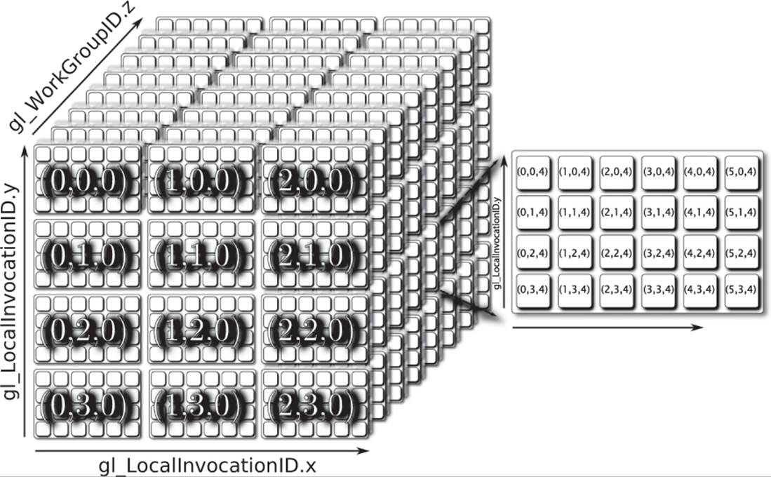
Figure 10.1: Global and local compute work group dimensions
Between gl_WorkGroupID and gl_LocalInvocationID, you can tell where in the complete set of work items your current shader invocation is located. Likewise, between gl_NumWorkGroups and gl_WorkGroupSize, you can figure out the total number of invocations in the global set. However, OpenGL provides the global invocation index to you through the gl_GlobalInvocationID built-in variable. This is effectively calculated as
gl_GlobalInvocationID = gl_WorkGroupID * gl_WorkGroupSize +
gl_LocalInvocationID;
Finally, the gl_LocalInvocationIndex built-in variable contains a “flattened” form of gl_LocalInvocationID. That is, the 3D variable is converted to a 1D index using the following code:
gl_LocalInvocationIndex =
gl_LocalInvocationID.z * gl_WorkGroupSize.x * gl_WorkGroupSize.y +
gl_LocalInvocationID.y * gl_WorkGroupSize.x +
gl_LocalInvocationID.x;
The values stored in these variables allow your shader to know where it is in the local and global work groups and can then be used as indices into arrays of data, texture coordinates, random seeds, or for any other purpose.
Now we come to outputs. We started this section by stating that compute shaders have no outputs. That’s true, but it doesn’t mean that compute shaders can’t output any data — it just means that there are no fixed outputs represented by built-in output variables, for example. Compute shaders can still produce data, but it must be stored into memory explicitly by your shader code. For instance, in your compute shader you could write into a shader storage block, use image functions such as imageStore or atomics, or increment and decrement the values of atomic counters. These operations have side effects, which means that their operation can be detected because they update the contents of memory or otherwise have externally visible consequences.
Consider the shader shown in Listing 10.2, which reads from one image, logically inverts the data, and writes the data back out to another image.
#version 430 core
layout (local_size_x = 32,
local_size_y = 32) in;
layout (binding = 0, rgba32f) uniform image2D img_input;
layout (binding = 1) uniform image2D img_output;
void main(void)
{
vec4 texel;
ivec2 p = ivec2(gl_GlobalInvocationID.xy);
texel = imageLoad(img_input, p);
texel = vec4(1.0) - texel;
imageStore(img_output, p, texel);
}
Listing 10.2: Compute shader image inversion
In order to execute this shader, we would compile it and link it into a program object and then set up our images by binding a level of a texture object to each of the first two image units. As you can see from Listing 10.2, the local work group size is 32 invocations in x and y, so our images should ideally be integer multiples of 32 texels wide and high. Once the images are bound, we can call glDispatchCompute(), setting the num_groups_x and num_groups_y parameters to the width and height of the images divided by 32, respectively, and setting num_groups_z to 1. Code to do this is shown in Listing 10.3.
// Bind input image
glBindImageTexture(0, tex_input, 0, GL_FALSE,
0, GL_READ_ONLY, GL_RGBA32F);
// Bind output image
glBindImageTexture(1, tex_output, 0, GL_FALSE,
0, GL_WRITE_ONLY, GL_RGBA32F);
// Dispatch the compute shader
glDispatchCompute(IMAGE_WIDTH / 32, IMAGE_HEIGHT / 32, 1);
Listing 10.3: Dispatching the image copy compute shader
Compute Shader Communication
Compute shaders execute on work items in work groups much as tessellation control shaders execute on control points in patches2 — both work groups and patches are created from groups of invocations. Within a single patch, tessellation control shaders can write to variables qualified with the patch storage qualifier and, if they are synchronized correctly, read the values that other invocations in the same patch wrote to them. As such, this allows a limited form of communication between the tessellation control shader invocations in a single patch. However, this comes with substantial limitations — for example, the amount of storage available for patch qualified variables is fairly limited, and the number of control points in a single patch is quite small.
2. This may also seem similar to the behavior of geometry shaders. However, there is an important difference — compute shaders and tessellation control shaders execute an invocation per work item or per control point, respectively. Geometry shaders, on the other hand, execute an invocation for each primitive, and each of those invocations has access to all of the input data for that primitive.
Compute shaders provide a similar mechanism, but offer significantly more flexibility and power. Just as you can declare variables with the patch storage qualifier in a tessellation control shader, you can declare variables with the shared storage qualifier, which allows them to be sharedbetween compute shader invocations running in the same local work group. Variables declared with the shared storage qualifier are known as shared variables. Access to shared variables is generally much faster than access to main memory through images or storage blocks. Thus, if you expect multiple invocations of your compute shader to access the same data, it makes sense to copy the data from main memory into a shared variable (or an array of them), access the data from there, possibly updating it in place, and then write any results back to main memory when you’re done.
Keep in mind, though, that you can only use a limited number of shared variables. A modern graphics board might have several gigabytes of main memory, whereas the amount of shared variable storage space might be limited to just a few kilobytes. The amount of shared memory available to a compute shader can be determined by calling glGetIntegerv() with pname set to GL_MAX_COMPUTE_SHARED_MEMORY_SIZE. The minimum amount of shared memory required to be supported in OpenGL is only 32KB, so while your implementation may have more than this, you shouldn’t count on it being substantially larger.
Synchronizing Compute Shaders
The invocations in a work group most likely run in parallel — this is where the vast computation power of graphics processors comes from. The processor will likely divide each local work group into a number of smaller3 chunks, executing the invocations in a single chunk in lockstep. These chunks are then time-sliced onto the processor’s computational resources, and those timeslices may be assigned in any order. It may be that a chunk of invocations is completed before any more chunks from the same local work group begin, but more than likely there will be many “live” chunks present on the processor at any given time.
3. Chunk sizes of 16, 32, or 64 elements are common.
Because these chunks can effectively run out of order but are allowed to communicate, we need a way to ensure that messages received by a recipient are the most recent sent. Imagine if you were told to go to someone’s office and perform the duty written on their whiteboard. Each day, they would write a new message on the whiteboard, but you don’t know at what time they do it. When you go into the office, how do you know if the message that’s there is what you’re supposed to do, or if it’s left over from the previous day? You’d be in a bit of trouble. Now, if the owner of the office left their door locked until they’d been there and written the message and then you showed up and the door was locked, you’d have to wait outside the office. This is known as a barrier. If the door is open, you can go look at the message. If it’s locked, you need to wait until the person arrives to open it.
A similar mechanism is available to compute shaders. This is the barrier() function, and it executes a flow control barrier. When you call barrier() in your compute shader, it will be blocked until all other shader invocations in the same local work group have reached that point in the shader too. We touched on this back in “Communication between Shader Invocations” in Chapter 8, where we described the behavior of the barrier() function in the context of tessellation control shaders. In a time-slicing architecture, executing the barrier() function means that your shader (along with the chunk it’s in) will give up its timeslice so that another invocation can execute until it reaches the barrier. Once all the other invocations in the local work group reach the barrier (or if they’d already gotten there before your invocation did) execution continues as normal.
Flow control barriers are important when shared memory is in use because they allow you to know when other shader invocations in the same local workgroup have reached the same point as the current invocation. If the current invocation has written to some shared memory variable, then you know that all the others must have written to theirs too, and therefore it’s safe to go ahead and read the data they wrote. Without a barrier, you would have no idea whether data that was supposed to have been written to shared variables actually has been. At best, you’d leave your application susceptible to race conditions, and at worst, the application won’t work at all. Consider, for example, the shader in Listing 10.4.
#version 430 core
layout (local_size_x = 1024) in;
layout (binding = 0, r32ui) uniform uimageBuffer image_in;
layout (binding = 1) uniform uimageBuffer image_out;
shared uint temp_storage[1024];
void main(void)
{
// Load from the input image
uint n = imageLoad(image_in, gl_LocalInvocationID.x).x;
// Store into shared storage
temp_storage[gl_LocalInvocationID.x] = n;
// Uncomment this to avoid the race condition
// barrier();
// memoryBarrierShared();
// Read the data written by the invocation "to the left"
n = temp_storage[(gl_LocalInvocationID.x - 1) & 1023];
// Write new data into the buffer
imageStore(image_out, gl_LocalInvocationID.x, n);
}
Listing 10.4: Compute shader with race conditions
This shader loads data from a buffer image into a shared variable. Each invocation of the shader loads a single item from the buffer and writes it into its own “slot” in the shared variable array. Then, it reads from the slot owned by the invocation to its left and writes the data out to the buffer image. The result should be that the data in the buffer is moved along by one element. However, Figure 10.2 illustrates what actually happens.
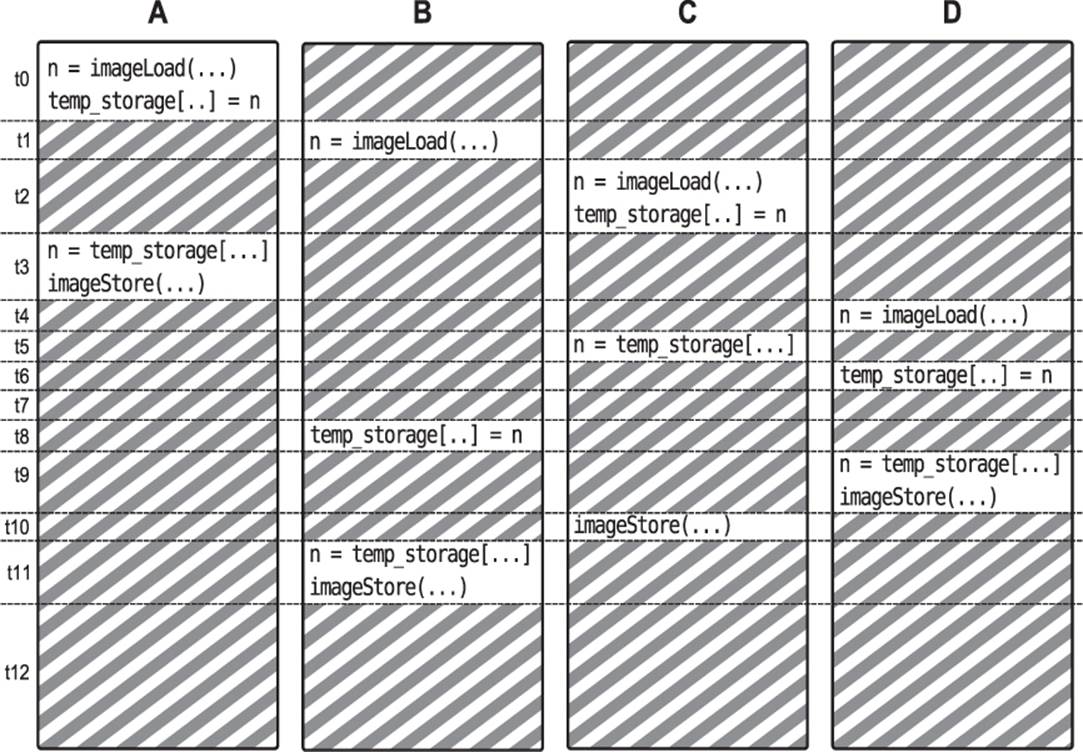
Figure 10.2: Effect of race conditions in a compute shader
As you can see, multiple shader invocations have been time-sliced onto a single computational resource. At t0, invocation A runs the first couple of lines of the shader and writes its value to temp_storage. At t1, invocation B runs a line, and then at t2, invocation C takes over and runs the same first two lines of the shader. At time t3, A gets its timeslice back again and completes the shader. It’s done at this point, but the other invocations haven’t finished their work yet. At t4, invocation D finally gets a turn but is quickly interrupted by invocation C, which reads fromtemp_storage. Now we have a problem — invocation C was expecting to read data from the shared storage that was written by invocation B, but invocation B hasn’t reached that point in the shader yet! Execution continues blindly, and invocations D, C, and B all finish the shader, but the data stored by C will be garbage.
This is known as a race condition. The shader invocations race each other to the same point in the shader, and some invocations will read from the temp_storage shared variable before others have written their data into it. The result is that they pick up stale data that then gets written into the output buffer image. Uncommenting the call to barrier() in Listing 10.4 produces an execution flow more like that shown in Figure 10.3.
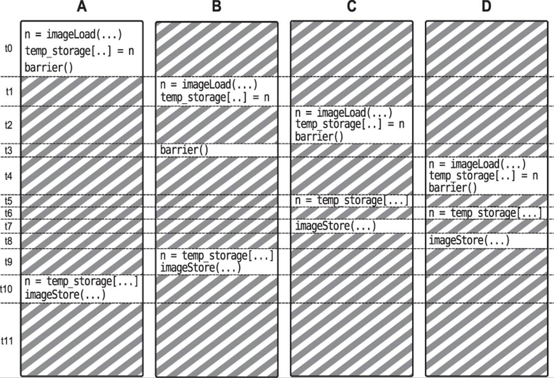
Figure 10.3: Effect of barrier() on race conditions
Compare Figures 10.2 and 10.3. Both depict four shader invocations being time-sliced onto the same computational resource, only Figure 10.3 does not exhibit the race condition. In Figure 10.3, we again start with shader invocation A executing the first couple of lines of the shader, but then it calls the barrier() function, which causes it to yield its timeslice. Next, invocation B executes the first couple of lines and then is pre-empted. Then, C executes the shader as far as the barrier() function and so yields. Invocation B executes its barrier but gets no further because D still has not reached the barrier function. Finally, invocation D gets a chance to run, reads from the image buffer, writes its data into the shared storage area, and then calls barrier(). This signals all the other invocations that it is safe to continue running.
Immediately after invocation D executes the barrier, all other invocations are able to run again. Invocation C loads from the shared storage, then D, and then C and D both store their results to the image. Finally, invocations A and B read from the shared storage and write their results out to memory. As you can see, no invocation tried to read data that hasn’t been written yet. The presence of the barrier() functions affected the scheduling of the invocations with respect to one another. Although these diagrams show only four invocations competing for a single resource, in real OpenGL implementations there are likely to be many hundreds of threads competing for perhaps a few tens of resources. As you might guess, the likelihood of data corruption due to race conditions is much higher in these scenarios.
Examples
The following section contains several examples of the use of compute shaders. In our first example, the parallel prefix sum, we demonstrate how to implement an algorithm (which at first seems like a very serial process) in an efficient parallel manner. In our second example, an implementation of the classic flocking algorithm (also known as boids) is shown. In both examples, we make use of local and global work groups, synchronization using the barrier() command, and shared local variables — a feature unique to compute shaders.
Compute Shader Parallel Prefix Sum
A prefix sum operation is an algorithm that, given an array of input values, computes a new array where each element of the output array is the sum of all of the values of the input array up to (and optionally including) the current array element. A prefix sum operation that includes the current element is known as an inclusive prefix sum, and one that does not is known as an exclusive prefix sum. For example, the code shown in Listing 10.5 shows a simple C++ implementation of a prefix sum function that can be inclusive or exclusive.
void prefix_sum(const float * in_array,
float * out_array,
int elements,
bool inclusive)
{
float f = 0.0f;
int i;
if (inclusive)
{
for (i = 0; i < elements; i++)
{
f += in_array[i];
out_array[i] = f;
}
}
else
{
for (i = 0; i < elements; i++)
{
out_array[i] = f;
f += in_array[i];
}
}
}
Listing 10.5: Simple prefix sum implementation in C++
Notice that the only difference between the inclusive and exclusive prefix sum implementations is that the accumulation of the input array is conducted before writing to the output array rather than afterwards. The result of running an inclusive prefix sum on an array of values is illustrated inFigure 10.4.
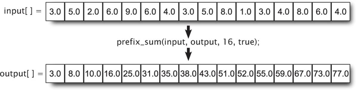
Figure 10.4: Sample input and output of a prefix sum operation
You should appreciate that as the number of elements in the input and output arrays grows, the number of addition operations grows too and can become quite large. Also, as the result written to each element of the output array is the sum of all elements before it (and therefore dependent on all of them), it would seem at first glance that this type of algorithm does not lend itself well to parallelization. However, this is not the case — the prefix sum operation is highly parallelizable. At its core, the prefix sum is nothing more than a huge number of additions of adjacent array elements. Take, for example, a prefix sum of four input elements, I0 through I3, producing an output array O0 through O3. The result is
O0 = I0
O1 = I0 + I1
O2 = I0 + I1 + I2
O3 = I0 + I1 + I2 + I3
The key to parallelization is to break large tasks into groups of smaller, independent tasks that can be completed independently of one another. Now, you can see that in the computation of O2 and O3, we use the sum of I0 and I1, which we also need to calculate O1. So, if we break this operation into multiple steps, we see that we have in the first step
O0 = I0
O1 = I0 + I1
O2 = I2
O3 = I2 + I3
Then, in a second step, we can compute
O2 = O2 + O1
O3 = O3 + O1
Now, the computations of O1 and O3 are independent of one another in the first step and therefore can be computed in parallel as can the updates of the values of O2 and O3 in the second step. If you look closely, you will see that the first step simply takes a four-element prefix sum and breaks it into a pair of two-element prefix sums that are trivially computed. In the second step, we use the result of the previous to update the results of the inner sums. In fact, we can break any sized prefix sum into smaller and smaller chunks until we reach a point where we can compute the inner sum directly. This is shown pictorially in Figure 10.5.
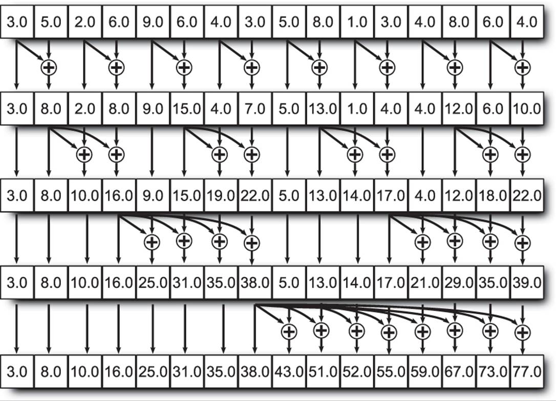
Figure 10.5: Breaking a prefix sum into smaller chunks
The recursive nature of this algorithm is apparent in Figure 10.5. The number of additions required by this method is actually more than the sequential algorithm for prefix sum calculation would require. In this example, we would require 15 additions to compute the prefix sum with a sequential algorithm, whereas here we require 8 additions per step and 4 steps for a total of 32 additions. However, we can execute the 8 additions of each step in parallel, and hence we will be done in 4 steps instead of 15, making the algorithm almost 4 times faster than the sequential one.
As the number of elements in the input array grows, the potential speedup becomes greater. For example, if we expand the input array to 32 elements, we execute 5 steps of 16 additions each rather than 31 sequential additions. Assuming we have enough computational resources to perform 16 additions at a time, we now take 5 steps instead of 31 and go around 6 times faster. Likewise, for an input array size of 64, we’d take 6 steps of 32 additions rather than 63 sequential additions, and go 10 times faster! Of course, we eventually hit a limit in either the number of additions we can perform in parallel, the amount of memory bandwidth we consume reading and writing the input and output arrays, or something else.
To implement this in a compute shader, we can load a chunk of input data into shared variables, compute the inner sums, synchronize with the other invocations, accumulate their results, and so on. An example compute shader that implements this algorithm is shown in Listing 10.6.
#version 430 core
layout (local_size_x = 1024) in;
layout (binding = 0) coherent buffer block1
{
float input_data[gl_WorkGroupSize.x];
};
layout (binding = 1) coherent buffer block2
{
float output_data[gl_WorkGroupSize.x];
};
shared float shared_data[gl_WorkGroupSize.x * 2];
void main(void)
{
uint id = gl_LocalInvocationID.x;
uint rd_id;
uint wr_id;
uint mask;
// The number of steps is the log base 2 of the
// work group size, which should be a power of 2
const uint steps = uint(log2(gl_WorkGroupSize.x)) + 1;
uint step = 0;
// Each invocation is responsible for the content of
// two elements of the output array
shared_data[id * 2] = input_data[id * 2];
shared_data[id * 2 + 1] = input_data[id * 2 + 1];
// Synchronize to make sure that everyone has initialized
// their elements of shared_data[] with data loaded from
// the input arrays
barrier();
memoryBarrierShared();
// For each step...
for (step = 0; step < steps; step++)
{
// Calculate the read and write index in the
// shared array
mask = (1 << step) - 1;
rd_id = ((id >> step) << (step + 1)) + mask;
wr_id = rd_id + 1 + (id & mask);
// Accumulate the read data into our element
shared_data[wr_id] += shared_data[rd_id];
// Synchronize again to make sure that everyone
// has caught up with us
barrier();
memoryBarrierShared();
}
// Finally write our data back to the output image
output_data[id * 2] = shared_data[id * 2];
output_data[id * 2 + 1] = shared_data[id * 2 + 1];
}
Listing 10.6: Prefix sum implementation using a compute shader
The shader shown in Listing 10.6 has a local workgroup size of 1024, which means it will process arrays of 2048 elements, as each invocation computes two elements of the output array. The shared variable shared_data is used to store the data that is in flight, and at the start of execution, the shader loads two adjacent elements from the input arrays into the array. Next, it executes the barrier() function. This is to ensure that all of the shader invocations have loaded their data into the shared array before the inner loop begins.
Each iteration of the inner loop performs one step of the algorithm. This loop executes log2(N) times, where N is the number of elements in the array. For each invocation, the shader calculates the index of the first and second elements to be added together and then computes the sum, writing the result back into the shared array. At the end of the loop, there is another call to barrier(), which ensures that the invocations are fully synchronized before the next iteration of the loop and ultimately when the loop exits. Finally, it writes the result to the output buffer.
Prefix sum algorithms can be applied in a separable manner to multi-dimensional data sets such as images and volumes. You have already seen an example of a separable algorithm when we performed Gaussian filtering in our bloom example back in Chapter 9. To produce a prefix sum of an image, we would first apply our prefix sum algorithm across each row of pixels in the image, producing a new image, and then apply another prefix sum on each of the columns of the at result. The output of these two steps is a new 2D grid where each point represents the sum of all of the values contained in the rectangle whose corners are at the origin and at the point of interest. Figure 10.6 demonstrates the principle.
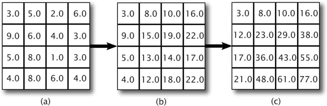
Figure 10.6: A 2D prefix sum
As you can see, given the input in Figure 10.6 (a), the first step simply computes a number of prefix sums over the rows of the image, producing an output image that is comprised of a set of prefix sums shown in Figure 10.6 (b). The second step performs prefix sum operations on the columns of the intermediate image, producing an output containing the 2D prefix sum of the original image, shown in Figure 10.6 (c). Such an image is called a summed area table, and is an extremely important data structure with many applications in computer graphics.
We can modify our shader of Listing 10.6 to compute the prefix sums of the rows of an image variable rather than a shader storage buffer. The modified shader is shown in Listing 10.7. As an optimization, the shader reads from the input image’s rows but writes to the images columns. This means that the output image will be transposed with respect to the input. However, we’re going to apply this shader twice, and we know that transposing an image twice returns it to its original orientation, which means that the final result will be correctly oriented with respect to the original input. Also, if we wanted to avoid the transpose operation, the shader to process the rows would need to be different from the shader that processes the columns (or do extra work to figure out how to index the image). With this approach, the shader for both passes is identical.
#version 430 core
layout (local_size_x = 1024) in;
shared float shared_data[gl_WorkGroupSize.x * 2];
layout (binding = 0, r32f) readonly uniform image2D input_image;
layout (binding = 1, r32f) writeonly uniform image2D output_image;
void main(void)
{
uint id = gl_LocalInvocationID.x;
uint rd_id;
uint wr_id;
uint mask;
ivec2 P = ivec2(id * 2, gl_WorkGroupID.x);
const uint steps = uint(log2(gl_WorkGroupSize.x)) + 1;
uint step = 0;
shared_data[id * 2] = imageLoad(input_image, P).r;
shared_data[id * 2 + 1] = imageLoad(input_image,
P + ivec2(1, 0)).r;
barrier();
memoryBarrierShared();
for (step = 0; step < steps; step++)
{
mask = (1 << step) - 1;
rd_id = ((id >> step) << (step + 1)) + mask;
wr_id = rd_id + 1 + (id & mask);
shared_data[wr_id] += shared_data[rd_id];
barrier();
memoryBarrierShared();
}
imageStore(output_image, P.yx, vec4(shared_data[id * 2]));
imageStore(output_image, P.yx + ivec2(0, 1),
vec4(shared_data[id * 2 + 1]));
}
Listing 10.7: Compute shader to generate a 2D prefix sum
Each local work group of the shader in Listing 10.7 is still one dimensional. However, when we launch the shader for the first pass, we create a one-dimensional global work group containing as many local work groups as there are rows in the image, and then when we launch it for the second pass, we create as many local work groups as there are columns in the image (which are actually rows again at this point due to the transpose operation performed by the shader). Each local work group will therefore process the row or column of the image determined by the global workgroup index.
Given a summed area table for an image, we can actually compute the sum of the elements contained within an arbitrary rectangle of that image. To do this, we simply need four values from the table, each one giving the sum of the elements contained within the rectangle spanning from the origin to its coordinate. Given a rectangle of interest defined by an upper-left and lower-right coordinate, we add the values from the summed area table at the upper-left and lower-right coordinates, and then subtract the values at its upper-right and lower-left coordinates. To see why this works, refer to Figure 10.7.
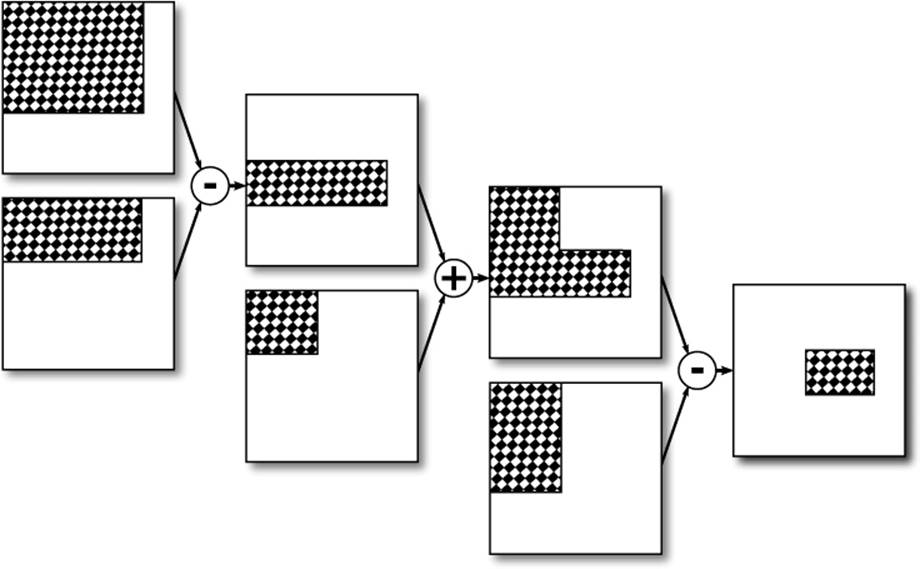
Figure 10.7: Computing the sum of a rectangle in a summed area table
Now, the number of pixels contained in any given rectangle of the summed area table is simply the rectangle’s area. Given this, we know that if we take the sum of all the elements contained with the rectangle and divide this through by its area, we will be left with the average value of the elements inside the rectangle. Averaging a number of values together is a form of filtering known as a box filter, and while it’s pretty crude, it can be useful for certain applications. In particular, being able to take the average of an arbitrary number of pixels centered around an arbitrary point in an image allows us to create a variable-sized filter, where the dimensions of the filtered rectangle can be changed per pixel.
As an example, Figure 10.8 shows an image that has a variable-sized filter applied to it. The image is least heavily filtered on the left and more heavily filtered on the right. As you can see, the right side of the image is substantially more blurry than the left side of it.
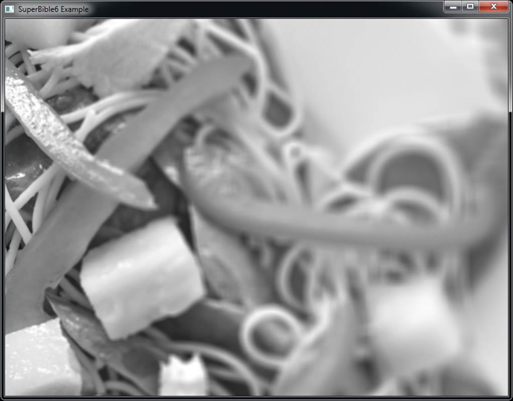
Figure 10.8: Variable filtering applied to an image
Simple filtering effects like this are great, but we can use this same technique to generate some much more interesting results. One such effect is the depth of field effect. Cameras have two properties that are relevant to this effect — focal distance and focal depth. The focal distance refers to the distance from the camera at which an object must be placed to be perfectly in focus. The focal depth refers to the rate at which an object becomes out of focus as it moves away from this sweet spot.
An example of this is seen in the photograph4 shown in Figure 10.9. The glass closest to the camera is in sharp focus. However, as the row of glasses progresses from front to back, they become successively less well defined. The basket of oranges in the background is quite out of focus. The true blur of an image due to out of focus lenses is caused by a number of complex optical phenomena, but we can make a pretty good approximation to the visual effect with our rudimentary box filter.
4. Photograph courtesy of http://www.cookthestory.com.

Figure 10.9: Depth of field in a photograph
To simulate our depth of field effect, we’ll first render our scene as normal, but save the depth of each fragment (which is approximately equal to its distance from the camera). When this depth value is equal to our simulated camera’s focal distance, the image will be sharp and in focus, as it normally is with computer graphics. As the depth of a pixel strays from this perfect depth, the amount of blur we apply to the image should increase too.
We have implemented this in the dof sample. In the program, we convert the rendered image into a summed area table using the compute shader shown in Listing 10.7, modified slightly to operate on vec3 data rather than a single floating-point value per pixel. Also, as we rendered the image, we stored the per-pixel view-space depth in the fourth alpha channel of the image so that our fragment shader, shown in Listing 10.8, would have access to it. The fragment shader then computes the area of confusion (which is a fancy term for the size of the blurred size) for the current pixel and uses it to build a filter width (m), reading data from the summed area table to produce blurry pixels.
#version 430 core
layout (binding = 0) uniform sampler2D input_image;
layout (location = 0) out vec4 color;
uniform float focal_distance = 50.0;
uniform float focal_depth = 30.0;
void main(void)
{
// s will be used to scale our texture coordinates before
// looking up data in our SAT image.
vec2 s = 1.0 / textureSize(input_image, 0);
// C is the center of the filter
vec2 C = gl_FragCoord.xy;
// First, retrieve the value of the SAT at the center
// of the filter. The last channel of this value stores
// the view-space depth of the pixel.
vec4 v = texelFetch(input_image, ivec2(gl_FragCoord.xy), 0).rgba;
// M will be the radius of our filter kernel
float m;
// For this application, we clear our depth image to zero
// before rendering to it, so if it's still zero, we haven't
// rendered to the image here. Thus, we set our radius to
// 0.5 (i.e., a diameter of 1.0) and move on.
if (v.w == 0.0)
{
m = 0.5;
}
else
{
// Calculate a circle of confusion
m = abs(v.w - focal_distance);
// Simple smoothstep scale and bias. Minimum radius is
// 0.5 (diameter 1.0), maximum is 8.0. Box filter kernels
// greater than about 16 pixels don't look good at all.
m = 0.5 + smoothstep(0.0, focal_depth, m) * 7.5;
}
// Calculate the positions of the four corners of our
// area to sample from.
vec2 P0 = vec2(C * 1.0) + vec2(-m, -m);
vec2 P1 = vec2(C * 1.0) + vec2(-m, m);
vec2 P2 = vec2(C * 1.0) + vec2(m, -m);
vec2 P3 = vec2(C * 1.0) + vec2(m, m);
// Scale our coordinates.
P0 *= s;
P1 *= s;
P2 *= s;
P3 *= s;
// Fetch the values of the SAT at the four corners
vec3 a = textureLod(input_image, P0, 0).rgb;
vec3 b = textureLod(input_image, P1, 0).rgb;
vec3 c = textureLod(input_image, P2, 0).rgb;
vec3 d = textureLod(input_image, P3, 0).rgb;
// Calculate the sum of all pixels inside the kernel.
vec3 f = a - b - c + d;
// Scale radius -> diameter.
m *= 2;
// Divide through by area
f /= float(m * m);
// Output final color
color = vec4(f, 1.0);
}
Listing 10.8: Depth of field using summed area tables
The shader in Listing 10.8 takes as input a texture containing the depth of each pixel and the summed area table of the image computed earlier, along with the parameters of the simulated camera. As the absolute value of the difference between the pixel’s depth and the camera’s focal distance increases, it uses this value to compute the size of the filtering rectangle (which is known as the area of confusion). It then reads the four values from the summed area table at the corners of the rectangle, computes the average value of its content, and writes this to the framebuffer. The result is that pixels that are “further” from the ideal focal distance are blurred more and pixels that are closer to it are blurred less. The result of this shader is shown in Figure 10.10. This image is also shown in Color Plate 8.
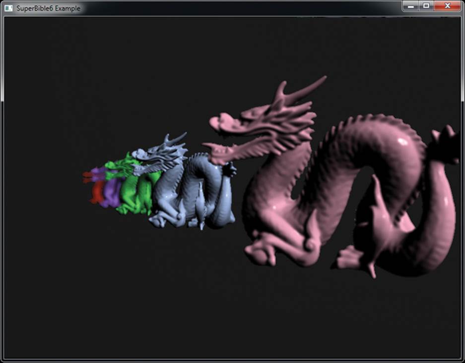
Figure 10.10: Applying depth of field to an image
As you can see in Figure 10.10, the depth of field effect has been applied to a row of dragons. In the image, the nearest dragon appears slightly blurred and out of focus, the second dragon is in focus, and the dragons beyond it become successively out of focus again. Figure 10.11 shows several more results from the same program. In the leftmost image of Figure 10.11, the closest dragon is in sharp focus, and the furthest dragon is very blurry. In the middle image of Figure 10.11, the furthest dragon is the one in focus, whereas the closest is the most blurred. To achieve this effect, the depth of field of the simulated camera is quite shallow. By lengthening the camera’s depth of field, we can obtain the image on the right of Figure 10.11, where the effect is far more subtle. However, all three images were produced in real time using the same program and varying only two parameters — the focal distance and the depth of field.
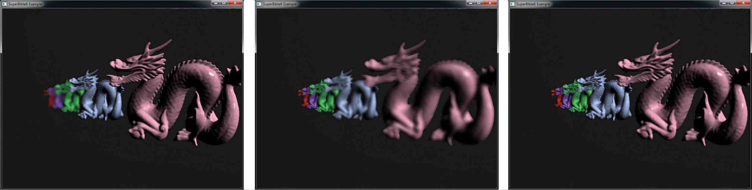
Figure 10.11: Effects achievable with depth of field
In order to simplify this example, we used 32-bit floating-point data for every component of every image. This allows us to not worry about precision issues. Because the precision of floating-point data gets lower as the magnitude of the data gets higher, summed area tables can suffer from precision loss. As the values of all of the pixels in the image are summed together, the values stored in the summed area tables can become very large. Then, as the output image is reconstructed, the difference between multiple (potentially large valued) floating-point numbers is taken, which can lead to noise.
In order to improve our implementation of the algorithm, we could
• Render our initial image in 16-bit floating point rather than at full 32-bit precision.
• Store the depth of our fragments in a separate texture (or reconstruct them from the depth buffer), eliminating the need to store them in the intermediate image.
• Pre-bias our rendered image by −0.5, which keeps the summed area table values closer to zero even for larger images, thereby improving precision.
Compute Shader Flocking
The following example uses a compute shader to implement a flocking algorithm. Flocking algorithms show emergent behavior within a large group by updating the properties of individual members independently of all others. This kind of behavior is regularly seen in nature, and examples are swarms of bees, flocks of birds, and schools of fish apparently moving in unison even though the members of the group don’t communicate globally. That is, the decisions made by an individual are based solely on its perception of the other nearby members of the group. However, no collaboration is made between members over the outcome of any particular decision — as far as we know, schools of fish don’t have leaders. Because each member of the group is effectively independent, the new value of each of the properties can be calculated in parallel — ideal for a GPU implementation.
Here, we implement the flocking algorithm in a compute shader. We represent each member of the flock as a single element stored in a shader storage buffer. Each member has a position and a velocity that are updated by a compute shader that reads the current values from one buffer and writes the result into another buffer. That buffer is then bound as a vertex buffer and used as an instanced input to the rendering vertex shader. Each member of the flock is an instance in the rendering draw. The vertex shader is responsible for transforming a mesh (in this case, a simple model of a paper airplane) into the position and orientation calculated in the first vertex shader. The algorithm then iterates, starting again with the compute shader, reusing the positions and velocities calculated in the previous pass. No data leaves the graphics card’s memory, and the CPU is not involved in any calculations.
We use a pair of buffers to store the current position of the members of the flock. We also use a set of VAOs to represent the vertex array state for each pass so that we can render the resulting data. These VAOs also hold the vertex data for the model we use to represent them. The flock positions and velocities need to be double-buffered because we don’t want to partially update the position or velocity buffer while at the same time using them as a source for drawing commands. Figure 10.12 illustrates the passes that the algorithm makes.
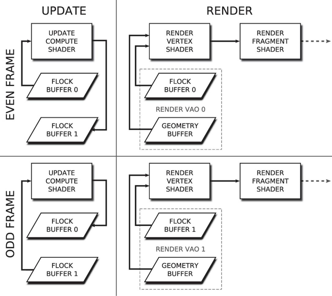
Figure 10.12: Stages in the iterative flocking algorithm
On the top left, we perform the update for an even frame. The first buffer containing position and velocity is bound as a shader storage buffer that can be read by the compute shader, and the second buffer is bound such that it can be written by the compute shader. Next we render, on the top right of Figure 10.12, using the same set of buffers as inputs as in the update pass. We use the same buffers as input in both the update and render passes so that the render pass has no dependency on the update pass. That means that OpenGL may be able to start working on the render pass before the update pass has finished. The buffer containing the position and velocity of the flock members is used to source instanced vertex attributes, and the additional geometry buffer is used to provide vertex position data.
On the bottom left of Figure 10.12, we move to the next frame. The buffers have been exchanged—the second buffer is now the input to the compute shader, and the first is written by it. Finally, on the bottom right of Figure 10.12, we render the odd frames. The second buffer is used as input to the vertex shader. Notice, though, that the flock_geometry buffer is a member of both rendering VAOs because the same data is used in both passes, and so we don’t need two copies of it.
The code to set all that up is shown in Listing 10.9. It isn’t particularly complex, but there is a fair amount of repetition, making it long. The listing contains the bulk of the initialization.
glGenBuffers(2, flock_buffer);
glBindBuffer(GL_SHADER_STORAGE_BUFFER, flock_buffer[0]);
glBufferData(GL_SHADER_STORAGE_BUFFER,
FLOCK_SIZE * sizeof(flock_member),
NULL,
GL_DYNAMIC_COPY);
glBindBuffer(GL_SHADER_STORAGE_BUFFER, flock_buffer[1]);
glBufferData(GL_SHADER_STORAGE_BUFFER,
FLOCK_SIZE * sizeof(flock_member),
NULL,
GL_DYNAMIC_COPY);
glGenBuffers(1, &geometry_buffer);
glBindBuffer(GL_ARRAY_BUFFER, geometry_buffer);
glBufferData(GL_ARRAY_BUFFER, sizeof(geometry), geometry, GL_STATIC_DRAW);
glGenVertexArrays(2, flock_render_vao);
for (i = 0; i < 2; i++)
{
glBindVertexArray(flock_render_vao[i]);
glBindBuffer(GL_ARRAY_BUFFER, geometry_buffer);
glVertexAttribPointer(0, 3, GL_FLOAT, GL_FALSE,
0, NULL);
glVertexAttribPointer(1, 3, GL_FLOAT, GL_FALSE,
0, (void *)(8 * sizeof(vmath::vec3)));
glBindBuffer(GL_ARRAY_BUFFER, flock_buffer[i]);
glVertexAttribPointer(2, 3, GL_FLOAT, GL_FALSE,
sizeof(flock_member), NULL);
glVertexAttribPointer(3, 3, GL_FLOAT, GL_FALSE,
sizeof(flock_member),
(void *)sizeof(vmath::vec4));
glVertexAttribDivisor(2, 1);
glVertexAttribDivisor(3, 1);
glEnableVertexAttribArray(0);
glEnableVertexAttribArray(1);
glEnableVertexAttribArray(2);
glEnableVertexAttribArray(3);
}
Listing 10.9: Initializing shader storage buffers for flocking
In addition to running the code shown in Listing 10.9, we initialize our flock positions with some random vectors and set all of the velocities to zero.
Now we need a rendering loop to update our flock positions and draw the members of the flock. It’s actually pretty simple now that we have our data encapsulated in VAOs. The rendering loop is shown in Listing 10.10. You can clearly see the two passes that the loop makes. First, theupdate_program is made current and used to update the positions and velocities of the flock members. The position of the goal is updated, the storage buffers are bound to the first and second GL_SHADER_STORAGE_BUFFER binding points for reading and writing, and then the compute shader is dispatched.
Next, the window is cleared, the rendering program is activated, and we update our transform matrices, bind our VAO, and draw. The number of instances is the number of members of our simulated flock, and the number of vertices is simply the amount of geometry we’re using to represent our little paper airplane.
glUseProgram(flock_update_program);
vmath::vec3 goal = vmath::vec3(sinf(t * 0.34f),
cosf(t * 0.29f),
sinf(t * 0.12f) * cosf(t * 0.5f));
goal = goal * vmath::vec3(15.0f, 15.0f, 180.0f);
glUniform3fv(uniforms.update.goal, 1, goal);
glBindBufferBase(GL_SHADER_STORAGE_BUFFER, 0, flock_buffer[frame_index]);
glBindBufferBase(GL_SHADER_STORAGE_BUFFER, 1, flock_buffer[frame_index ^ 1]);
glDispatchCompute(NUM_WORKGROUPS, 1, 1);
glViewport(0, 0, info.windowWidth, info.windowHeight);
glClearBufferfv(GL_COLOR, 0, black);
glClearBufferfv(GL_DEPTH, 0, &one);
glUseProgram(flock_render_program);
vmath::mat4 mv_matrix =
vmath::lookat(vmath::vec3(0.0f, 0.0f, -400.0f),
vmath::vec3(0.0f, 0.0f, 0.0f),
vmath::vec3(0.0f, 1.0f, 0.0f));
vmath::mat4 proj_matrix =
vmath::perspective(60.0f,
(float)info.windowWidth / (float)info.windowHeight,
0.1f,
3000.0f);
vmath::mat4 mvp = proj_matrix * mv_matrix;
glUniformMatrix4fv(uniforms.render.mvp, 1, GL_FALSE, mvp);
glBindVertexArray(flock_render_vao[frame_index]);
glDrawArraysInstanced(GL_TRIANGLE_STRIP, 0, 8, FLOCK_SIZE);
frame_index ^= 1;
Listing 10.10: The rendering loop for the flocking example
That’s pretty much the interesting part of the program side. Let’s take a look at the shader side of things. The flocking algorithm works by applying a set of rules for each member of the flock to decide which direction to travel in. Each rule considers the current properties of the flock member and the properties of the other members of the flock as perceived by the individual being updated. Most of the rules require access to the other member’s position and velocity data, so update_program uses a shader storage buffer containing that information. Listing 10.11 shows the start of the update compute shader. It lists the uniforms we’ll use5 during simulation, the declaration of the flock member, the two buffers used for input and output, and, finally, a shared array of members that will be used during the updates.
5. Most of these uniforms are not hooked up to the example program, but their default values can be changed by tweaking the shader.
#version 430 core
layout (local_size_x = 256) in;
uniform float closest_allowed_dist2 = 50.0;
uniform float rule1_weight = 0.18;
uniform float rule2_weight = 0.05;
uniform float rule3_weight = 0.17;
uniform float rule4_weight = 0.02;
uniform vec3 goal = vec3(0.0);
uniform float timestep = 0.5;
struct flock_member
{
vec3 position;
vec3 velocity;
};
layout (std430, binding = 0) buffer members_in
{
flock_member member[];
} input_data;
layout (std430, binding = 1) buffer members_out
{
flock_member member[];
} output_data;
shared flock_member shared_member[gl_WorkGroupSize.x];
Listing 10.11: Compute shader for updates in flocking example
Once we have declared all of the inputs to our shader, we have to define our rules that we’re going to use to update them. The rules we use in this example are as follows:
• Members try not to hit each other. They need to stay at least a short distance from each other at all times.
• Members try to fly in the same direction as those around them.
• Members of the flock try to reach a common goal.
• Members try to keep with the rest of the flock. They will fly toward the center of the flock.
The first two rules are the intra-member rules. That is, the effect of each of the members on each other is considered individually. Listing 10.12 contains the shader code for the first rule. If we’re closer to another member than we’re supposed to be, we simply move away from that member.
vec3 rule1(vec3 my_position,
vec3 my_velocity,
vec3 their_position,
vec3 their_velocity)
{
vec3 d = my_position - their_position;
if (dot(d, d) < closest_allowed_dist2)
return d;
return vec3(0.0);
}
Listing 10.12: The first rule of flocking
The shader for the second rule is shown in Listing 10.13. It returns a change in velocity weighted by the inverse square of the distance from each member to the member. A small amount is added to the squared distance between the members to keep the denominator of the fraction from getting too small (and thus the acceleration too large), which keeps the simulation stable.
vec3 rule2(vec3 my_position,
vec3 my_velocity,
vec3 their_position,
vec3 their_velocity)
{
vec3 d = their_position - my_position;
vec3 dv = their_velocity - my_velocity;
return dv / (dot(d, d) + 10.0);
}
Listing 10.13: The second rule of flocking
The third rule (that flock members attempt to fly towards a common goal) is applied once per member. The fourth rule (that members attempt to get to the center of the flock) is also applied once per member, but requires the average position of all of the flock members (along with the total number of members in the flock) to calculate.
The main body of the program contains the meat of the algorithm. The flock is broken into groups and each group is represented as a single local workgroup (the size of which we have defined as 256 elements). Because every member of the flock needs to interact in some way with every other member of the flock, this algorithm is considered an O(N2) algorithm. This means that each of the N flock members will read all of the other N members’ positions and velocities, and that each of the N members’ positions and velocities will be read N times. Rather than read through the entirety of the input shader storage buffer for every flock member, we copy a local workgroup’s worth of data into a shared storage buffer and use the local copy to update each of the members.
For each flock member (which is a single invocation of our compute shader), we loop over the number of work groups and copy a single flock member’s data into the shared local copy (the shared_member array declared at the top of the shader in Listing 10.11). Each of the 256 local shader invocations copies one element into the shared array and then executes the barrier() function to ensure that all of the invocations are synchronized and have therefore copied their data into the shared array. Then, we loop over all of the data stored in the shared array, apply each of the intra-member rules in turn, sum up the resulting vector, and then execute another call to barrier(). This again synchronizes the threads in the local workgroup and ensures that all of the other invocations have finished using the shared array before we restart the loop and write over it again. Code to do this is given in Listing 10.14.
void main(void)
{
uint i, j;
int global_id = int(gl_GlobalInvocationID.x);
int local_id = int(gl_LocalInvocationID.x);
flock_member me = input_data.member[global_id];
flock_member new_me;
vec3 acceleration = vec3(0.0);
vec3 flock_center = vec3(0.0);
for (i = 0; i < gl_NumWorkGroups.x; i++)
{
flock_member them =
input_data.member[i * gl_WorkGroupSize.x +
local_id];
shared_member[local_id] = them;
memoryBarrierShared();
barrier();
for (j = 0; j < gl_WorkGroupSize.x; j++)
{
them = shared_member[j];
flock_center += them.position;
if (i * gl_WorkGroupSize.x + j != global_id)
{
acceleration += rule1(me.position,
me.velocity,
them.position,
them.velocity) * rule1_weight;
acceleration += rule2(me.position,
me.velocity,
them.position,
them.velocity) * rule2_weight;
}
}
barrier();
}
flock_center /= float(gl_NumWorkGroups.x * gl_WorkGroupSize.x);
new_me.position = me.position + me.velocity * timestep;
acceleration += normalize(goal - me.position) * rule3_weight;
acceleration += normalize(flock_center - me.position) * rule4_weight;
new_me.velocity = me.velocity + acceleration * timestep;
if (length(new_me.velocity) > 10.0)
new_me.velocity = normalize(new_me.velocity) * 10.0;
new_me.velocity = mix(me.velocity, new_me.velocity, 0.4);
output_data.member[global_id] = new_me;
}
Listing 10.14: Main body of the flocking update compute shader
In addition to applying the first two rules on a per-member basis and then adjusting acceleration to try to get the members to fly towards the common goal and towards the center of the flock, we also apply a couple more rules to keep the simulation sane. First, if the velocity of the flock member gets too high, we clamp it to a maximum allowed value. Second, rather than output the new velocity verbatim, we perform a weighted average between it and the old velocity. This forms a basic low-pass filter and stops the flock members from accelerating or decelerating too quickly or, more importantly, from changing direction too abruptly.
Putting all this together completes the update phase of the program. Now we need to produce the shaders that are responsible for rendering the flock. This program uses the position and velocity data calculated by the compute shader as instanced vertex arrays and transforms a fixed set of vertices into position based on the position and velocity of the individual member. Listing 10.15 shows the inputs to the shader.
#version 430 core
layout (location = 0) in vec3 position;
layout (location = 1) in vec3 normal;
layout (location = 2) in vec3 bird_position;
layout (location = 3) in vec3 bird_velocity;
out VS_OUT
{
flat vec3 color;
} vs_out;
uniform mat4 mvp;
Listing 10.15: Inputs to the flock rendering vertex shader
In this shader, position and normal are regular inputs from our geometry buffer, which in this example contains a simple model of a paper airplane. The bird_position and bird_velocity inputs will be the instanced attributes, provided by the compute shader and whose instance divisor is set with the glVertexAttribDivisor() function. The body of our shader (given in Listing 10.16) uses the velocity of the flock member to construct a lookat matrix that can be used to orient the airplane model such that it’s always flying forward.
mat4 make_lookat(vec3 forward, vec3 up)
{
vec3 side = cross(forward, up);
vec3 u_frame = cross(side, forward);
return mat4(vec4(side, 0.0),
vec4(u_frame, 0.0),
vec4(forward, 0.0),
vec4(0.0, 0.0, 0.0, 1.0));
}
vec3 choose_color(float f)
{
float R = sin(f * 6.2831853);
float G = sin((f + 0.3333) * 6.2831853);
float B = sin((f + 0.6666) * 6.2831853);
return vec3(R, G, B) * 0.25 + vec3(0.75);
}
void main(void)
{
mat4 lookat = make_lookat(normalize(bird_velocity),
vec3(0.0, 1.0, 0.0));
vec4 obj_coord = lookat * vec4(position.xyz, 1.0);
gl_Position = mvp * (obj_coord + vec4(bird_position, 0.0));
vec3 N = mat3(lookat) * normal;
vec3 C = choose_color(fract(float(gl_InstanceID / float(1237.0))));
vs_out.color = mix(C * 0.2, C, smoothstep(0.0, 0.8, abs(N).z));
}
Listing 10.16: Flocking vertex shader body
Construction of the lookat matrix uses a method similar to that described in Chapter 4, “Math for 3D Graphics.” Once we have oriented the mesh using this matrix, we add the flock member’s position and transform the whole lot by the model-view-projection matrix. We also orient the object’s normal by the lookat matrix, which allows us to apply a very simple lighting calculation. We choose a color for the object based on the current instance ID (which is unique per mesh) and use it to compute the final output color, which we write into the vertex shader output. The fragment shader is a simple pass-through shader that writes this incoming color to the framebuffer. The result of rendering the flock is shown in Figure 10.13.
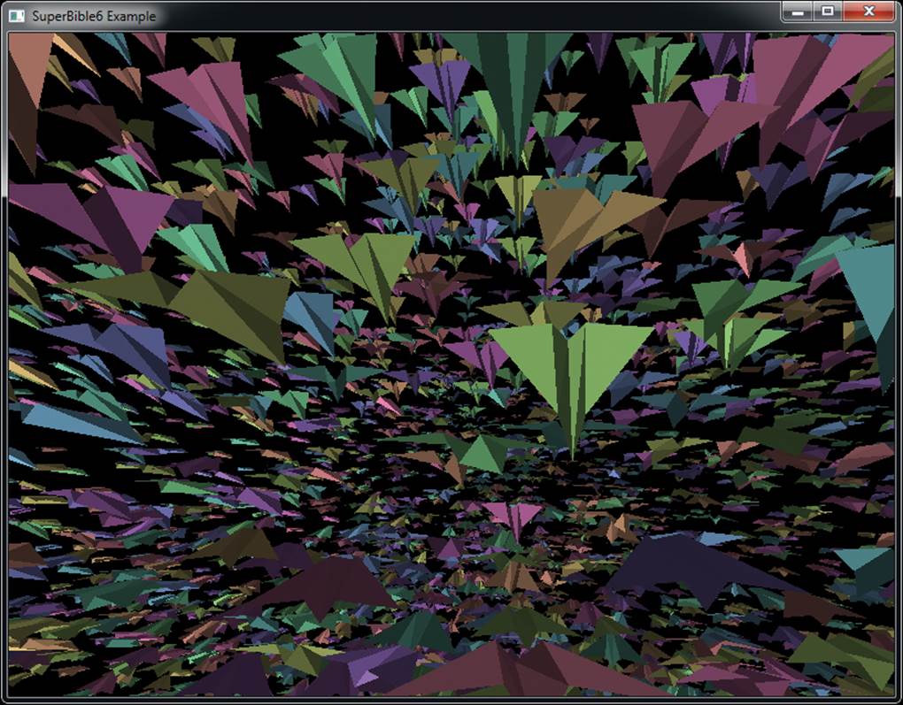
Figure 10.13: Output of compute shader flocking program
A possible enhancement that could be made to this program is to calculate the lookat matrix in the compute shader. Here, we calculate it in the vertex shader and therefore redundantly calculate it for every vertex. It doesn’t matter so much in this example because our mesh is small, but if our instanced mesh were larger, generating it in the compute shader and passing it along with the other instanced vertex attributes would likely be faster. We could also apply more physical simulations rather than just ad-hoc rules. For example, we could simulate gravity, making it easier to fly down than up, or we could allow the planes to crash into and bounce off of one another. However, for the purposes of this example, what we have here is sufficient.
Summary
In this chapter, we have taken an in-depth look at compute shaders — the “single-stage pipeline” that allows you to harness the computational power of modern graphics processors for more than just computer graphics. We have covered the execution model of compute shaders where you learned about work groups, synchronization, and intra-workgroup communication. Then, we covered some of the applications of compute shaders. First, we showed you the applications of compute shaders in image processing, which is an obvious fit for computer graphics. Next, we showed you how you might use compute shaders for physical simulation when we implemented the flocking algorithm. This should have allowed you to imagine some of the possibilities for the use of compute shaders in your own applications — from artificial intelligence, pre- and post-processing, or even audio applications!
All materials on the site are licensed Creative Commons Attribution-Sharealike 3.0 Unported CC BY-SA 3.0 & GNU Free Documentation License (GFDL)
If you are the copyright holder of any material contained on our site and intend to remove it, please contact our site administrator for approval.
© 2016-2026 All site design rights belong to S.Y.A.