OpenGL SuperBible: Comprehensive Tutorial and Reference, Sixth Edition (2013)
Part I: Foundations
Chapter 5. Data
What You’ll Learn in This Chapter
• How to create buffers and textures that you can use to store data that your program can access
• How to get OpenGL to supply the values of your vertex attributes automatically
• How to access textures from your shaders for both reading and writing
In the examples you’ve seen so far, we have either used hard-coded data directly in our shaders, or we have passed values to shaders one at a time. While sufficient to demonstrate the configuration of the OpenGL pipeline, this is hardly representative of modern graphics programming. Recent graphics processors are designed as streaming processors that consume and produce huge amounts of data. Passing a few values to OpenGL at a time is extremely inefficient. To allow data to be stored and accessed by OpenGL, we include two main forms of data storage — buffers and textures. In this chapter, we first introduce buffers, which are linear blocks of un-typed data and can be seen as generic memory allocations. Next, we introduce textures, which are normally used to store multi-dimensional data, such as images or other data types.
Buffers
In OpenGL, buffers are linear allocations of memory that can be used for a number of purposes. They are represented by names, which are essentially opaque handles that OpenGL uses to identify them. Before you can start using buffers, you have to ask OpenGL to reserve some names for you and then use them to allocate memory and put data into that memory. The memory allocated for a buffer object is called its data store. Once you have the name of a buffer, you can attach it to the OpenGL context by binding it to a buffer binding point. Binding points are sometimes referred to as targets,1 and the terms may be used interchangeably. There are a large number of buffer binding points in OpenGL, and each has a different use. For example, you can use the contents of a buffer to automatically supply the inputs of a vertex shader, to store the values of variables that will be used by your shaders, or as a place for shaders to store the data they produce.
1. It’s not technically correct to conflate target and binding point as a single target may have multiple binding points. However, for most use cases, it is well understood what is meant.
Allocating Memory using Buffers
The function that is used to allocate memory using a buffer object is glBufferData(), whose prototype is
void glBufferData(GLenum target,
GLsizeiptr size,
const GLvoid * data,
GLenum usage);
The target parameter tells OpenGL which target the buffer you want to allocate storage for is bound to. For example, the binding point that is used when you want to use a buffer to store data that OpenGL can put into your vertex attributes is called the GL_ARRAY_BUFFER binding point. Although you may hear the term vertex buffer or uniform buffer, unlike some graphics libraries, OpenGL doesn’t really assign types to buffers — a buffer is just a buffer and can be used for any purpose at any time (and even multiple purposes at the same time, if you like). The size parameter tells OpenGL how big the buffer should be, and data is a pointer to some initial data for the buffer (it can be NULL if you don’t have data to put in the buffer right away). Finally, usage tells OpenGL how you plan to use the buffer. There are a number of possible values for usage, which are listed in Table 5.1.
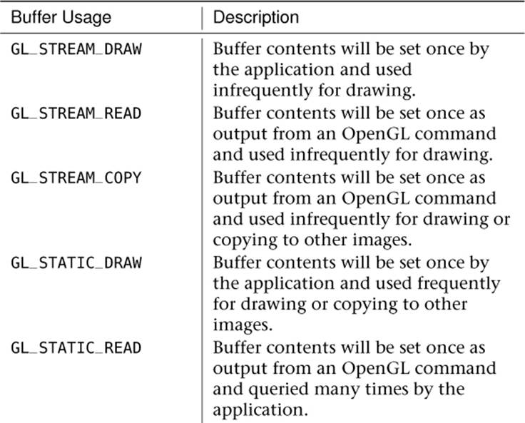
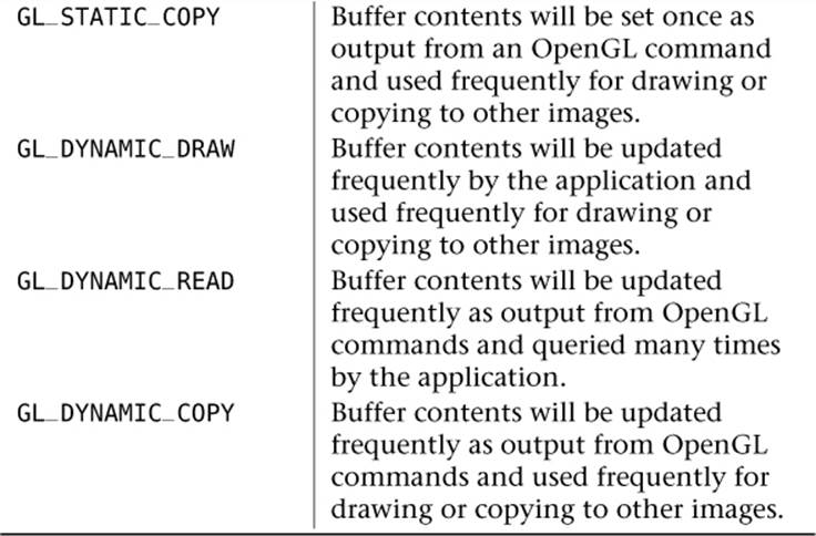
Table 5.1. Buffer Object Usage Models
Listing 5.1 shows how a name for a buffer is reserved by calling glGenBuffers(), how it is bound to the context using glBindBuffer(), and how storage for it is allocated by calling glBufferData().
// The type used for names in OpenGL is GLuint
GLuint buffer;
// Generate a name for the buffer
glGenBuffers(1, &buffer);
// Now bind it to the context using the GL_ARRAY_BUFFER binding point
glBindBuffer(GL_ARRAY_BUFFER, buffer);
// Specify the amount of storage we want to use for the buffer
glBufferData(GL_ARRAY_BUFFER, 1024 * 1024, NULL, GL_STATIC_DRAW);
Listing 5.1: Generating, binding, and initializing a buffer
After the code in Listing 5.1 has executed, buffer contains the name of a buffer object that has been initialized to represent one megabyte of storage for whatever data we choose. Using the GL_ARRAY_BUFFER target to refer to the buffer object suggests to OpenGL that we’re planning to use this buffer to store vertex data, but we’ll still be able to take that buffer and bind it to some other target later. There are a handful of ways to get data into the buffer object. You may have noticed the NULL pointer that we pass as the third argument to glBufferData() in Listing 5.1. Had we instead supplied a pointer to some data, that data would have been used to initialize the buffer object. Another way to get data into a buffer is to give it to OpenGL and tell it to copy data there. To do this, we call glBufferSubData(), passing the size of the data we want to put into the buffer, the offset in the buffer where we want it to go, and a pointer to the data in memory that should be put into the buffer. glBufferSubData() is declared as
void glBufferSubData(GLenum target,
GLintptr offset,
GLsizeiptr size,
const GLvoid * data);
Listing 5.2 shows how we can put the data originally used in Listing 3.1 into a buffer object, which is the first step in automatically feeding a vertex shader with data.
// This is the data that we will place into the buffer object
static const float data[] =
{
0.25, -0.25, 0.5, 1.0,
-0.25, -0.25, 0.5, 1.0,
0.25, 0.25, 0.5, 1.0
};
// Put the data into the buffer at offset zero
glBufferSubData(GL_ARRAY_BUFFER, 0, sizeof(data), data);
Listing 5.2: Updating the content of a buffer with glBufferSubData()
Another method for getting data into a buffer object is to ask OpenGL for a pointer to the memory that the buffer object represents and then copy the data there yourself. Listing 5.3 shows how to do this using the glMapBuffer() function.
// This is the data that we will place into the buffer object
static const float data[] =
{
0.25, -0.25, 0.5, 1.0,
-0.25, -0.25, 0.5, 1.0,
0.25, 0.25, 0.5, 1.0
};
// Get a pointer to the buffer's data store
void * ptr = glMapBuffer(GL_ARRAY_BUFFER, GL_WRITE_ONLY);
// Copy our data into it...
memcpy(ptr, data, sizeof(data));
// Tell OpenGL that we're done with the pointer
glUnmapBuffer(GL_ARRAY_BUFFER);
Listing 5.3: Mapping a buffer’s data store with glMapBuffer()
The glMapBuffer() function is useful if you don’t have all the data handy when you call the function. For example, you might be about to generate the data, or to read it from a file. If you wanted to use glBufferSubData() (or the initial pointer passed to glBufferData()), you’d have to generate or read the data into a temporary memory and then get OpenGL to make another copy of it into the buffer object. If you map a buffer, you can simply read the contents of the file directly into the mapped buffer. When you unmap it, if OpenGL can avoid making a copy of the data, it will. Regardless of whether we used glBufferSubData() or glMapBuffer() and an explicit copy to get data into our buffer object, it now contains a copy of data[] and we can use it as a source of data to feed our vertex shader.
Filling and Copying Data in Buffers
After allocating storage space for your buffer object using glBufferData(), one possible next step is to fill the buffer with known data. Whether you use the initial data parameter of glBufferData(), use glBufferSubData() to put the initial data in the buffer, or use glMapBuffer() to obtain a pointer to the buffer’s data store and fill it with your application, you will need to overwrite the entire buffer. If the data you want to put into a buffer is a constant value, it is probably much more efficient to call glClearBufferSubData(), whose prototype is
void glClearBufferSubData(GLenum target,
GLenum internalformat,
GLintptr offset,
GLsizeiptr size,
GLenum format,
GLenum type,
const void * data);
The glClearBufferSubData() function takes a pointer to a variable containing the values that you want to clear the buffer object to and, after converting it to the format specified in internalformat, replicates it across the range of the buffer’s data store specified by offset and size, both of which are measured in bytes. format and type tell OpenGL about the data pointed to by data. Format can be one of GL_RED, GL_RG, GL_RGB, or GL_RGBA to specify 1-, 2-, 3-, or 4-channel data, for example. Meanwhile, type should represent the data type of the components. For instance, it could beGL_UNSIGNED_BYTE or GL_FLOAT to specify unsigned bytes or floating-point data. The most common types supported by OpenGL and their corresponding C data types are listed in Table 5.2.
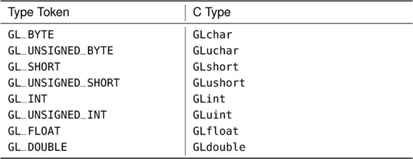
Table 5.2. Basic OpenGL Type Tokens and Their Corresponding C Types
Once your data has been sent to the GPU, it’s entirely possible you may want to share that data between buffers or copy the results from one buffer into another. OpenGL provides an easy-to-use way of doing that. glCopyBufferSubData() lets you specify which buffers are involved as well as the size and offsets to use.
void glCopyBufferSubData(GLenum readtarget,
GLenum writetarget,
GLintptr readoffset,
GLintptr writeoffset,
GLsizeiptr size);
The readtarget and writetarget are the targets where the two buffers you want to copy data between are bound. These can be buffers bound to any of the available buffer binding points. However, since buffer binding points can only have one buffer bound at a time, you couldn’t copy between two buffers both bound to the GL_ARRAY_BUFFER target, for example. This means that when you perform the copy, you need to pick two targets to bind the buffers to, which will disturb OpenGL state.
To resolve this, OpenGL provides the GL_COPY_READ_BUFFER and GL_COPY_WRITE_BUFFER targets. These targets were added specifically to allow you to copy data from one buffer to another without any unintended side effects. They are not used for anything else in OpenGL, and so you can bind your read and write buffers to these binding points without affecting any other buffer target. The readoffset and writeoffset parameters tell OpenGL where in the source and destination buffers to read or write the data, and the size parameter tells it how big the copy should be. Be sure that the ranges you are reading from and writing to remain within the bounds of the buffers; otherwise, your copy will fail.
You may notice the types of readoffset, writeoffset, and size, which are GLintptr and GLsizeiptr. These types are special definitions of integer types that are at least wide enough to hold a pointer variable.
Feeding Vertex Shaders from Buffers
Back in Chapter 2, you were briefly introduced to the vertex array object (VAO) where we explained how it represented the inputs to the vertex shader — even though at the time, we didn’t use any real inputs to our vertex shaders and opted instead for hard-coded arrays of data. Then, inChapter 3 we introduced the concept of vertex attributes, but we only discussed how to change their static values. Although the vertex array object stores these static attribute values for you, it can do a whole lot more. Before we can proceed, we need to create a vertex array object to store our vertex array state:
GLuint vao;
glGenVertexArrays(1, &vao);
glBindVertexArray(vao);
Now that we have our VAO created and bound, we can start filling in its state. Rather than using hard-coded data in the vertex shader, we can instead rely entirely on the value of a vertex attribute and ask OpenGL to fill it automatically using the data stored in a buffer object that we supply. To tell OpenGL where in the buffer object our data is, we use the glVertexAttribPointer() function2 to describe the data, and then enable automatic filling of the attribute by calling glEnableVertexAttribArray(). The prototypes of glVertexAttribPointer() andglEnableVertexAttribArray() are
2. glVertexAttribPointer() is so named for historical reasons. Way back in times of yore, OpenGL didn’t have buffer objects and all of the data it read was from your application’s memory. When you called glVertexAttribPointer(), you really did give it a pointer to real data. On modern architectures, that’s horribly inefficient, especially if the data will be read more than once, and so now OpenGL only supports reading data from buffer objects. Although the name of the function remains to this day, the pointer parameter is really interpreted as an offset into a buffer object.
void glVertexAttribPointer(GLuint index,
GLint size,
GLenum type,
GLboolean normalized,
GLsizei stride,
const GLvoid * pointer);
void glEnableVertexAttribArray(GLuint index);
For glVertexAttribPointer(), the first parameter, index, is the index of the vertex attribute. You can define a large number of attributes as input to a vertex shader and then refer to them by their index as explained in “Vertex Attributes” in Chapter 3. size is the number of components that are stored in the buffer for each vertex, and type is the type of the data, which would normally be one of the types in Table 5.2.
The normalized parameter tells OpenGL whether the data in the buffer should be normalized (scaled between 0.0 and 1.0) before being passed to the vertex shader or if it should be left alone and passed as is. This is ignored for floating-point data, but for integer data types such asGL_UNSIGNED_BYTE or GL_INT, it is important. For example, if GL_UNSIGNED_BYTE data is normalized, it is divided by 255 (the maximum value representable by an unsigned byte) before being passed to a floating-point input to the vertex shader. The shader will therefore see values of the input attribute between 0.0 and 1.0. However, if the data is not normalized, it is simply casted to floating point and the shader will receive numbers between 0.0 and 255.0, even though the input to the vertex shader is floating-point.
The stride parameter tells OpenGL how many bytes are between the start of one vertex’s data and the start of the next, but you can set this to zero to let OpenGL calculate it for you based on the values of size and type.
Finally, pointer is, despite its name, the offset into the buffer that is currently bound to GL_ARRAY_BUFFER where the vertex attribute’s data starts.
An example showing how to use glVertexAttribPointer() to configure a vertex attribute is shown in Listing 5.4. Notice that we also call glEnableVertexAttribArray() after setting up the pointer. This tells OpenGL to use the data in the buffer to fill the vertex attribute rather than using data we give it using one of the glVertexAttrib*() functions.
// First, bind our buffer object to the GL_ARRAY_BUFFER binding
// The subsequent call to glVertexAttribPointer will reference this buffer
glBindBuffer(GL_ARRAY_BUFFER, buffer);
// Now, describe the data to OpenGL, tell it where it is, and turn on
// automatic vertex fetching for the specified attribute
glVertexAttribPointer(0, // Attribute 0
4, // Four components
GL_FLOAT, // Floating-point data
GL_FALSE, // Not normalized
// (floating-point data never is)
0, // Tightly packed
NULL); // Offset zero (NULL pointer)
glEnableVertexAttribArray(0);
Listing 5.4: Setting up a vertex attribute
After Listing 5.4 has been executed, OpenGL will automatically fill the first attribute in the vertex shader with data it has read from the buffer that was bound when glVertexAttribPointer() was called. We can modify our vertex shader to use only its input vertex attribute rather than a hard-coded array. This updated shader is shown in Listing 5.5.
#version 430 core
layout (location = 0) in vec4 position;
void main(void)
{
gl_Position = position;
}
Listing 5.5: Using an attribute in a vertex shader
As you can see, the shader of Listing 5.5 is greatly simplified over the original shader shown in Chapter 2. Gone is the hard-coded array of data, and as an added bonus, this shader can be used with an arbitrary number of vertices. You can literally put millions of vertices worth of data into your buffer object and draw them all with a single command such as a call to glDrawArrays().
If you are done using data from a buffer object to fill a vertex attribute, you can disable that attribute again with a call to glDisableVertexAttribArray(), whose prototype is
void glDisableAttribArray(GLuint index);
Once you have disabled the vertex attribute, it goes back to being static and passing the value you specify with glVertexAttrib*() to the shader.
Using Multiple Vertex Shader Inputs
As you have learned, you can get OpenGL to feed data into your vertex shaders for you and using data you’ve placed in buffer objects. You can also declare multiple inputs to your vertex shaders and assign each one a unique location that can be used to refer to it. Combining these things together means that you can get OpenGL to provide data to multiple vertex shader inputs simultaneously. Consider the input declarations to a vertex shader shown in Listing 5.6
layout (location = 0) in vec3 position;
layout (location = 1) in vec3 color;
Listing 5.6: Declaring two inputs to a vertex shader
If you have a linked program object whose vertex shader has multiple inputs, you can determine the locations of those inputs by calling
GLint glGetAttribLocation(GLuint program,
const GLchar * name);
Here, program is the name of the program object containing the vertex shader, and name is the name of the vertex attribute. In our example declarations of Listing 5.6, passing "position" to glGetAttribLocation() will cause it to return 0, and passing "color" will cause it to return 1. Passing something that is not the name of a vertex shader input will cause glGetAttribLocation() to return -1. Of course, if you always specify locations for your vertex attributes in your shader code, then glGetAttribLocation() should return whatever you specified. If you don’t specify locations in shader code, OpenGL will assign locations for you, and those locations will be returned by glGetAttribLocation().
There are two ways to connect vertex shader inputs to your application’s data, and they are referred to as separate attributes and interleaved attributes.
When attributes are separate, that means that they are either located in different buffers, or at least at different locations in the same buffer. For example, if you want to feed data into two vertex attributes, you could create two buffer objects, bind the first to the GL_ARRAY_BUFFER target and callglVertexAttribPointer(), then bind the second buffer to the GL_ARRAY_BUFFER target and call glVertexAttribPointer() again for the second attribute. Alternatively, you can place the data at different offsets within the same buffer, bind it to the GL_ARRAY_BUFFER target, then callglVertexAttribPointer() twice — once with the offset to the first chunk of data and then again with the offset of the second chunk of data. Code demonstrating this is shown in Listing 5.7
GLuint buffer[2];
static const GLfloat positions[] = { ... };
static const GLfloat colors[] = { ... };
// Get names for two buffers
glGenBuffers(2, &buffers);
// Bind the first and initialize it
glBindBuffer(GL_ARRAY_BUFFER, buffer[0]);
glBufferData(GL_ARRAY_BUFFER, sizeof(positions), positions, GL_STATIC_DRAW);
glVertexAttribPointer(0, 3, GL_FLOAT, GL_FALSE, 0, NULL);
glEnableVertexAttribArray(0);
// Bind the second and initialize it
glBindBuffer(GL_ARRAY_BUFFER, buffer[1]);
glBufferData(GL_ARRAY_BUFFER, sizeof(colors), colors, GL_STATIC_DRAW);
glVertexAttribPointer(1, 3, GL_FLOAT, GL_FALSE, 0, NULL);
glEnableVertexAttribArray(1);
Listing 5.7: Multiple separate vertex attributes
In both cases of separate attributes, we have used tightly packed arrays of data to feed both attributes. This is effectively structure-of-arrays (SoA) data. We have a set of tightly packed, independent arrays of data. However, it’s also possible to use an array-of-structures form of data. Consider how the following structure might represent a single vertex:
struct vertex
{
// Position
float x;
float y;
float z;
// Color
float r;
float g;
float b;
};
Now we have two inputs to our vertex shader (position and color) interleaved together in a single structure. Clearly, if we make an array of these structures, we have an array-of-structures (AoS) layout for our data. To represent this with calls to glVertexAttribPointer(), we have to use itsstride parameter. The stride parameter tells OpenGL how far apart in bytes the start each vertex’s data is. If we leave it as zero, it’s a signal to OpenGL that the data is tightly packed and that it can work it out for itself given the type and stride parameters. However, to use the vertexstructure declared above, we can simply use sizeof(vertex) for the stride parameter and everything will work out. Listing 5.8 shows the code to do this.
GLuint buffer;
static const vertex vertices[] = { ... };
// Allocate and initialize a buffer object
glGenBuffers(1, &buffer);
glBindBuffer(GL_ARRAY_BUFFER, buffer);
glBufferData(GL_ARRAY_BUFFER, sizeof(vertices), vertices, GL_STATIC_DRAW);
// Set up two vertex attributes - first positions
glVertexAttribPointer(0, 3, GL_FLOAT, GL_FALSE,
sizeof(vertex), (void *)offsetof(vertex, x));
glEnableVertexAttribArray(0);
// Now colors
glVertexAttribPointer(1, 3, GL_FLOAT, GL_FALSE,
sizeof(vertex), (void *)offsetof(vertex, r));
glEnableVertexAttribArray(1);
Listing 5.8: Multiple interleaved vertex attributes
Loading Objects from Files
As you can see, you could potentially use a large number of vertex attributes in a single vertex shader, and as we progress through various techniques, you will see that we’ll regularly use four or five, possibly more. Filling buffers with data to feed all of these attributes and then setting up the vertex array object and all of the vertex attribute pointers can be a chore. Further, encoding all of your geometry data directly in your application just simply isn’t practical for anything but the simplest models. Therefore, it makes sense to store model data in files and load it into your application. There are plenty of model file formats out there, and most modeling programs support several of the more common formats.
For the purpose of this book, we have devised a simple object file definition called an .SBM file that stores the information we need without being either too simple or too over-engineered. Complete documentation for the format is contained in Appendix B. The sb6 framework also includes a loader for this model format, called sb6::object. To load an object file, create an instance of sb6::object, and call its load function as follows:
sb6::object my_object;
my_object.load("filename.sbm");
If successful, the model will be loaded into the instance of sb6::object, and you will be able to render it. During loading, the class will create and set up the object’s vertex array object and then configure all of the vertex attributes contained in the model file. The class also includes a renderfunction that binds the object’s vertex array object and calls the appropriate drawing command. For example, calling
my_object.render();
will render a single copy of the object with the current shaders. In many of the examples in the remainder of this book, we’ll simply use our object loader to load object files (several of which are included with the book’s source code) and render them.
Uniforms
Although not really a form of storage, uniforms are an important way to get data into shaders and to hook them up to your application. You have already seen how to pass data to a vertex shader using vertex attributes, and you have seen how to pass data from stage to stage using interface blocks. Uniforms allow you to pass data directly from your application into any shader stage. There are two flavors of uniforms that depend on how they are declared. The first are uniforms declared in the default block, and the second are uniform blocks, whose values are stored in buffer objects. We will discuss both now.
Default Block Uniforms
While attributes are needed for per-vertex positions, surface normals, texture coordinates, and so on, a uniform is how we pass data into a shader that stays the same — is uniform — for an entire primitive batch or longer. Probably the single most common uniform for a vertex shader is the transformation matrix. We use transformation matrices in our vertex shaders to manipulate vertex positions and other vectors. Any shader variable can be specified as a uniform, and uniforms can be in any of the shader stages (even though we only talk about vertex and fragment shaders in this chapter). Making a uniform is as simple as placing the keyword uniform at the beginning of the variable declaration:
uniform float fTime;
uniform int iIndex;
uniform vec4 vColorValue;
uniform mat4 mvpMatrix;
Uniforms are always considered to be constant, and they cannot be assigned to by your shader code. However, you can initialize their default values at declaration time in a manner such as
uniform answer = 42;
If you declare the same uniform in multiple shader stages, each of those stages will “see” the same value of that uniform.
Arranging Your Uniforms
After a shader has been compiled and linked into a program object, you can use one of many functions defined by OpenGL to set their values (assuming you don’t want the defaults defined by the shader). Just as with vertex attributes, these functions refer to uniforms by their location within their program object. It is possible to specify the locations of uniforms in your shader code by using a location layout qualifier. When you do this, OpenGL will try to assign the locations that you specify to the uniforms in your shaders. The location layout qualifier looks like
layout (location = 17) uniform vec4 myUniform;
You’ll notice the similarity between the location layout qualifier for uniforms and the one we’ve used for vertex shader inputs. In this case, myUniform will be allocated to location 17. If you don’t specify a location for your uniforms in your shader code, OpenGL will automatically assign locations to them for you. You can figure out what locations were assigned by calling the glGetUniformLocation() function, whose prototype is
GLint glGetUniformLocation(GLuint program,
const GLchar* name);
This function returns a signed integer that represents the location of the variable named by name in the program specified by program. For example, to get the location of a uniform variable named vColorValue, we would do something like this:
GLint iLocation = glGetUniformLocation(myProgram, "vColorValue");
In the previous example, passing "myUniform" to glGetUniformLocation() would result in the value 17 being returned. If you know a priori where your uniforms are because you assigned locations to them in your shaders, then you don’t need to find them and you can avoid the calls toglGetUniformLocation(). This is the recommended way of doing things.
If the return value of glGetUniformLocation() is -1, it means the uniform name could not be located in the program. You should bear in mind that even if a shader compiles correctly, a uniform name may still “disappear” from the program if it is not used directly in at least one of the attached shaders — even if you assign it a location explicitly in your shader source code. You do not need to worry about uniform variables being optimized away, but if you declare a uniform and then do not use it, the compiler will toss it out. Also, know that shader variable names are case sensitive, so you must get the case right when you query their locations.
Setting Scalars and Vector Uniforms
OpenGL supports a large number of data types both in the shading language and in the API, and in order to allow you to pass all this data around, it includes a huge number of functions just for setting the value of uniforms. A single scalar or vector data type can be set with any of the following variations on the glUniform*() function:
void glUniform1f(GLint location, GLfloat v0);
void glUniform2f(GLint location, Glfloat v0, GLfloat v1);
void glUniform3f(GLint location, GLfloat v0, GLfloat v1,
GLfloat v2);
void glUniform4f(GLint location, GLfloat v0, GLfloat v1,
GLfloat v2, GLfloat v3);
void glUniform1i(GLint location, GLint v0);
void glUniform2i(GLint location, GLint v0, GLint v1);
void glUniform3i(GLint location, GLint v0, GLint v1,
GLint v2);
void glUniform4i(GLint location, GLint v0, GLint v1,
GLint v2, GLint v3);
void glUniform1ui(GLint location, GLuint v0);
void glUniform2ui(GLint location, GLuint v0, GLuint v1);
void glUniform3ui(GLint location, GLuint v0, GLuint v1,
GLuint v2);
void glUniform4ui(GLint location, GLuint v0, GLuint v1,
GLuint v2, GLint v3);
For example, consider the following four variables declared in a shader:
uniform float fTime;
uniform int iIndex;
uniform vec4 vColorValue;
uniform bool bSomeFlag;
To find and set these values in the shader, your C/C++ code might look something like this:
GLint locTime, locIndex, locColor, locFlag;
locTime = glGetUniformLocation(myShader, "fTime");
locIndex = glGetUniformLocation(myShader, "iIndex");
locColor = glGetUniformLocation(myShader, "vColorValue");
locFlag = glGetUniformLocation(myShader, "bSomeFlag");
...
...
glUseProgram(myShader);
glUniform1f(locTime, 45.2f);
glUniform1i(locIndex, 42);
glUniform4f(locColor, 1.0f, 0.0f, 0.0f, 1.0f);
glUniform1i(locFlag, GL_FALSE);
Note that we used an integer version of glUniform*() to pass in a bool value. Booleans can also be passed in as floats, with 0.0 representing false, and any non-zero value representing true.
Setting Uniform Arrays
The glUniform*() function also comes in flavors that take a pointer, potentially to an array of values.
void glUniform1fv(GLint location, GLuint count, const GLfloat* value);
void glUniform2fv(GLint location, GLuint count, const Glfloat* value);
void glUniform3fv(GLint location, GLuint count, const GLfloat* value);
void glUniform4fv(GLint location, GLuint count, const GLfloat* value);
void glUniform1iv(GLint location, GLuint count, const GLint* value);
void glUniform2iv(GLint location, GLuint count, const GLint* value);
void glUniform3iv(GLint location, GLuint count, const GLint* value);
void glUniform4iv(GLint location, GLuint count, const GLint* value);
void glUniform1uiv(GLint location, GLuint count, constGLuint* value);
void glUniform2uiv(GLint location, GLuint count, constGLuint* value);
void glUniform3uiv(GLint location, GLuint count, constGLuint* value);
void glUniform4uiv(GLint location, GLuint count, constGLuint* value);
Here, the count value represents how many elements are in each array of x number of components, where x is the number at the end of the function name. For example, if you had a uniform with four components, such as one shown here:
uniform vec4 vColor;
then in C/C++, you could represent this as an array of floats:
GLfloat vColor[4] = { 1.0f, 1.0f, 1.0f, 1.0f };
But this is a single array of four values, so passing it into the shader would look like this:
glUniform4fv(iColorLocation, 1, vColor);
On the other hand, if you had an array of color values in your shader,
uniform vec4 vColors[2];
then in C++, you could represent the data and pass it in like this:
GLfloat vColors[4][2] = { { 1.0f, 1.0f, 1.0f, 1.0f } ,
{ 1.0f, 0.0f, 0.0f, 1.0f } };
...
glUniform4fv(iColorLocation, 2, vColors);
At its simplest, you can set a single floating-point uniform like this:
GLfloat fValue = 45.2f;
glUniform1fv(iLocation, 1, &fValue);
Setting Uniform Matrices
Finally, we see how to set a matrix uniform. Shader matrix data types only come in the single and double-precision floating-point variety, and thus we have far less variation. The following functions set the values of 2 × 2, 3 × 3, and 4 × 4 single-precision floating-point matrix uniforms, respectively:
glUniformMatrix2fv(GLint location, GLuint count,
GLboolean transpose, const GLfloat *m);
glUniformMatrix3fv(GLint location, GLuint count,
GLboolean transpose, const GLfloat *m);
glUniformMatrix4fv(GLint location, GLuint count,
GLboolean transpose, const GLfloat *m);
Similarly, the following functions set the values of 2 × 2, 3 × 3, and 4 × 4 double-precision floating-point matrix uniforms:
glUniformMatrix2dv(GLint location, GLuint count,
GLboolean transpose, const GLdouble *m);
glUniformMatrix3dv(GLint location, GLuint count,
GLboolean transpose, const GLdouble *m);
glUniformMatrix4dv(GLint location, GLuint count,
GLboolean transpose, const GLdouble *m);
In all of these functions, the variable count represents the number of matrices stored at the pointer parameter m (yes, you can have arrays of matrices!). The Boolean flag transpose is set to GL_FALSE if the matrix is already stored in column-major ordering (the way OpenGL prefers). Setting this value to GL_TRUE causes the matrix to be transposed when it is copied into the shader. This might be useful if you are using a matrix library that uses a row-major matrix layout instead (for example, some other graphics APIs use row-major ordering and you may wish to use a library designed for one of them).
Uniform Blocks
Eventually, the shaders you’ll be writing will become very complex. Some of them will require a lot of constant data, and passing all this to the shader using uniforms can become quite inefficient. If you have a lot of shaders in an application, you’ll need to set up the uniforms for every one of those shaders, which means a lot of calls to the various glUniform*() functions. You’ll also need to keep track of which uniforms change. Some change for every object, some change once per frame, while others may only require initializing once for the whole application. This means that you either need to update different sets of uniforms in different places in your application (making it more complex to maintain) or update all the uniforms all the time (costing performance).
To alleviate the cost of all the glUniform*() calls, to make updating a large set of uniforms simpler, and to be able to easily share a set of uniforms between different programs, OpenGL allows you to combine a group of uniforms into a uniform block and store the whole block in a buffer object. The buffer object is just like any other that has been described earlier. You can quickly set the whole group of uniforms by either changing your buffer binding or overwriting the content of a bound buffer. You can also leave the buffer bound while you change programs, and the new program will see the current set of uniform values. This functionality is called the uniform buffer object, or UBO. In fact, the uniforms you’ve used up until now live in the default block. Any uniform declared at the global scope in a shader ends up in the default uniform block. You can’t keep the default block in a uniform buffer object; you need to create one or more named uniform blocks.
To declare a set of uniforms to be stored in a buffer object, you need to use a named uniform block in your shader. This looks a lot like the interface blocks described in the section “Interface Blocks” back in Chapter 3, but it uses the uniform keyword instead of in or out. Listing 5.9 shows what the code looks like in a shader.
uniform TransformBlock
{
float scale; // Global scale to apply to everything
vec3 translation; // Translation in X, Y, and Z
float rotation[3]; // Rotation around X, Y, and Z axes
mat4 projection_matrix; // A generalized projection matrix to apply
// after scale and rotate
} transform;
Listing 5.9: Example uniform block declaration
This code declares a uniform block whose name is TransformBlock. It also declares a single instance of the block called transform. Inside the shader, you can refer to the members of the block using its instance name, transform (e.g., transform.scale or transform.projection_matrix). However, to set up the data in the buffer object that you’ll use to back the block, you need to know the location of a member of the block, and for that, you need the block name, TransformBlock. If you wanted to have multiple instances of the block, each with its own buffer, you could maketransform an array. The members of the block will have the same locations within each block, but there will now be several instances of the block that you can refer to in the shader. Querying the location of members within a block is important when you want to fill the block with data, which is explained in the following section.
Building Uniform Blocks
Data accessed in the shader via named uniform blocks can be stored in buffer objects. In general, it is the application’s job to fill the buffer objects with data using functions like glBufferData() or glMapBuffer(). The question is, then, what is the data in the buffer supposed to look like? There are actually two possibilities here, and whichever one you choose is a trade-off.
The first method is to use a standard, agreed upon layout for the data. This means that your application can just copy data into the buffers and assume specific locations for members within the block — you can even store the data on disk ahead of time and simply read it straight into a buffer that’s been mapped using glMapBuffer(). The standard layout may leave some empty space between the various members of the block, making the buffer larger than it needs to be, and you might even trade some performance for this convenience, but even so, using the standard layout is probably safe in almost all situations.
Another alternative is to let OpenGL decide where it would like the data. This can produce the most efficient shaders, but it means that your application needs to figure out where to put the data so that OpenGL can read it. Under this scheme, the data stored in uniform buffers is arranged in ashared layout. This is the default layout and is what you get if you don’t explicitly ask OpenGL for something else. With the shared layout, the data in the buffer is laid out however OpenGL decides is best for runtime performance and access from the shader. This can sometimes allow for greater performance to be achieved by the shaders, but requires more work from the application. The reason this is called the shared layout is that while OpenGL has arranged the data within the buffer, that arrangement will be the same between multiple programs and shaders sharing the same declaration of the uniform block. This allows you to use the same buffer object with any program. To use the shared layout, the application must determine the locations within the buffer object of the members of the uniform block.
First, we’ll describe the standard layout, which is what we would recommend that you use for your shaders (even though it’s not the default). To tell OpenGL that you want to use the standard layout, you need to declare the uniform block with a layout qualifier. A declaration of ourTransformBlock uniform block, with the standard layout qualifier, std140, is shown in Listing 5.10.
layout(std140) uniform TransformBlock
{
float scale; // Global scale to apply to everything
vec3 translation; // Translation in X, Y, and Z
float rotation[3]; // Rotation around X, Y, and Z axes
mat4 projection_matrix; // A generalized projection matrix to
// apply after scale and rotate
} transform;
Listing 5.10: Declaring a uniform block with the std140 layout
Once a uniform block has been declared to use the standard, or std140, layout, each member of the block consumes a predefined amount of space in the buffer and begins at an offset that is predictable by following a set of rules. A summary of the rules is as follows:
Any type consuming N bytes in a buffer begins on an N-byte boundary within that buffer. That means that standard GLSL types such as int, float, and bool (which are all defined to be 32-bit or four-byte quantities) begin on multiples of four bytes. A vector of these types of length two always begins on a 2N-byte boundary. For example, that means a vec2, which is eight bytes long in memory, always starts on an eight-byte boundary. Three- and four-element vectors always start on a 4N-byte boundary; so vec3 and vec4 types start on 16-byte boundaries, for instance. Each member of an array of scalar or vector types (int s or vec3 s, for example) always start boundaries defined by these same rules, but rounded up to the alignment of a vec4. In particular, this means that arrays of anything but vec4 (and N × 4 matrices) won’t be tightly packed, but instead there will be a gap between each of the elements. Matrices are essentially treated like short arrays of vectors, and arrays of matrices are treated like very long arrays of vectors. Finally, structures and arrays of structures have additional packing requirements; the whole structure starts on the boundary required by its largest member, rounded up to the size of a vec4.
Particular attention must be paid to the difference between the std140 layout and the packing rules that are often followed by your C++ (or other application language) compiler of choice. In particular, an array in a uniform block is not necessarily tightly packed. This means that you can’t create, for example, an array of float in a uniform block and simply copy data from a C array into it because the data from the C array will be packed, and the data in the uniform block won’t be.
This all sounds complex, but it is logical and well defined, and allows a large range of graphics hardware to implement uniform buffer objects efficiently. Returning to our TransformBlock example, we can figure out the offsets of the members of the block within the buffer using these rules.Listing 5.11 shows an example of a uniform block declaration along with the offsets of its members.
layout(std140) uniform TransformBlock
{
// Member base alignment offset aligned offset
float scale; // 4 0 0
vec3 translation; // 16 4 16
float rotation[3]; // 16 28 32 (rotation[0])
// 48 (rotation[1])
// 64 (rotation[2])
mat4 projection_matrix; // 16 80 80 (column 0)
// 96 (column 1)
// 112 (column 2)
// 128 (column 3)
} transform;
Listing 5.11: Example of a uniform block with offsets
There is a complete example of the alignments of various types in the original ARB_uniform_buffer_object extension specification.
If you really want to use the shared layout, you can determine the offsets that OpenGL assigned to your block members. Each member of a uniform block has an index that is used to refer to it to find its size and location within the block. To get the index of a member of a uniform block, call
void glGetUniformIndices(GLuint program,
GLsizei uniformCount,
const GLchar ** uniformNames,
GLuint * uniformIndices);
This function allows you to get the indices of a large set of uniforms — perhaps even all of the uniforms in a program with a single call to OpenGL, even if they’re members of different blocks. It takes a count of the number of uniforms you’d like the indices for (uniformCount) and an array of uniform names (uniformNames) and puts their indices in an array for you (uniformIndices). Listing 5.12 contains an example of how you would retrieve the indices of the members of TransformBlock, which we declared earlier.
static const GLchar * uniformNames[4] =
{
"TransformBlock.scale",
"TransformBlock.translation",
"TransformBlock.rotation",
"TransformBlock.projection_matrix"
};
GLuint uniformIndices[4];
glGetUniformIndices(program, 4, uniformNames, uniformIndices);
Listing 5.12: Retrieving the indices of uniform block members
After this code has run, you have the indices of the four members of the uniform block in the uniformIndices array. Now that you have the indices, you can use them to find the locations of the block members within the buffer. To do this, call
void glGetActiveUniformsiv(GLuint program,
GLsizei uniformCount,
const GLuint * uniformIndices,
GLenum pname,
GLint * params);
This function can give you a lot of information about specific uniform block members. The information that we’re interested in is the offset of the member within the buffer, the array stride (for TransformBlock.rotation), and the matrix stride (for TransformBlock.projection_matrix). These values tell us where to put data within the buffer so that it can be seen in the shader. We can retrieve these from OpenGL by setting pname to GL_UNIFORM_OFFSET, GL_UNIFORM_ARRAY_STRIDE, and GL_UNIFORM_MATRIX_STRIDE, respectively. Listing 5.13 shows what the code looks like.
GLint uniformOffsets[4];
GLint arrayStrides[4];
GLint matrixStrides[4];
glGetActiveUniformsiv(program, 4, uniformIndices,
GL_UNIFORM_OFFSET, uniformOffsets);
glGetActiveUniformsiv(program, 4, uniformIndices,
GL_UNIFORM_ARRAY_STRIDE, arrayStrides);
glGetActiveUniformsiv(program, 4, uniformIndices,
GL_UNIFORM_MATRIX_STRIDE, matrixStrides);
Listing 5.13: Retrieving the information about uniform block members
Once the code in Listing 5.13 has run, uniformOffsets contains the offsets of the members of the TransformBlock block, arrayStrides contains the strides of the array members (only rotation, for now), and matrixStrides contains the strides of the matrix members (only projection_matrix).
The other information that you can find out about uniform block members includes the data type of the uniform, the size in bytes that it consumes in memory, and layout information related to arrays and matrices within the block. You need some of that information to initialize a buffer object with more complex types, although the size and types of the members should be known to you already if you wrote the shaders. The other accepted values for pname and what you get back are listed in Table 5.3.
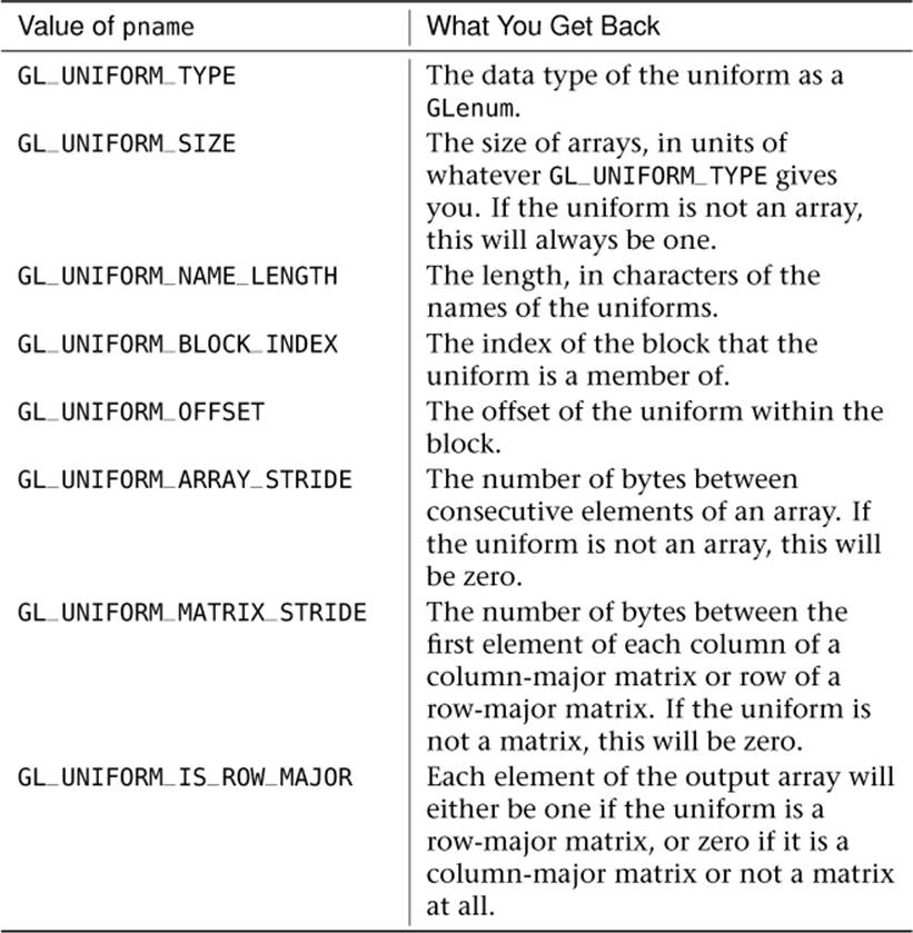
Table 5.3. Uniform Parameter Queries via glGetActiveUniformsiv()
If the type of the uniform you’re interested in is a simple type such as int, float, bool, or even vectors of these types (vec4 and so on), all you need is its offset. Once you know the location of the uniform within the buffer, you can either pass the offset to glBufferSubData() to load the data at the appropriate location, or you can use the offset directly in your code to assemble the buffer in memory. We demonstrate the latter option here because it reinforces the idea that the uniforms are stored in memory, just like vertex information can be stored in buffers. It also means fewer calls to OpenGL, which can sometimes lead to higher performance. For these examples, we assemble the data in the application’s memory and then load it into a buffer using glBufferData(). You could alternatively use glMapBuffer() to get a pointer to the buffer’s memory and assemble the data directly into that.
Let’s start by setting the simplest uniform in the TransformBlock block, scale. This uniform is a single float whose location is stored in the first element of our uniformIndices array. Listing 5.14 shows how to set the value of the single float.
// Allocate some memory for our buffer (don't forget to free it later)
unsigned char * buffer = (unsigned char *)malloc(4096);
// We know that TransformBlock.scale is at uniformOffsets[0] bytes
// into the block, so we can offset our buffer pointer by that value and
// store the scale there.
*((float *)(buffer + uniformOffsets[0])) = 3.0f;
Listing 5.14: Setting a single float in a uniform block
Next, we can initialize data for TransformBlock.translation. This is a vec3, which means it consists of three floating-point values packed tightly together in memory. To update this, all we need to do is find the location of the first element of the vector and store three consecutive floats in memory starting there. This is shown in Listing 5.15.
// Put three consecutive GLfloat values in memory to update a vec3
((float *)(buffer + uniformOffsets[1]))[0] = 1.0f;
((float *)(buffer + uniformOffsets[1]))[1] = 2.0f;
((float *)(buffer + uniformOffsets[1]))[2] = 3.0f;
Listing 5.15: Retrieving the indices of uniform block members
Now, we tackle the array rotation. We could have also used a vec3 here, but for the purposes of this example, we use a three-element array to demonstrate the use of the GL_UNIFORM_ARRAY_STRIDE parameter. When the shared layout is used, arrays are defined as a sequence of elements separated by an implementation-defined stride in bytes. This means that we have to place the data at locations in the buffer defined both by GL_UNIFORM_OFFSET and GL_UNIFORM_ARRAY_STRIDE, as in the code snippet of Listing 5.16.
// TransformBlock.rotations[0] is at uniformOffsets[2] bytes into
// the buffer. Each element of the array is at a multiple of
// arrayStrides[2] bytes past that
const GLfloat rotations[] = { 30.0f, 40.0f, 60.0f };
unsigned int offset = uniformOffsets[2];
for (int n = 0; n < 3; n++)
{
*((float *)(buffer + offset)) = rotations[n];
offset += arrayStrides[2];
}
Listing 5.16: Specifying the data for an array in a uniform block
Finally, we set up the data for TransformBlock.projection_matrix. Matrices in uniform blocks behave much like arrays of vectors. For column-major matrices (which is the default), each column of the matrix is treated like a vector, the length of which is the height of the matrix. Likewise, row-major matrices are treated like an array of vectors where each row is an element in that array. Just like normal arrays, the starting offset for each column (or row) in the matrix is determined by an implementation defined quantity. This can be queried by passing theGL_UNIFORM_MATRIX_STRIDE parameter to glGetActiveUniformsiv(). Each column of the matrix can be initialized using similar code to that which was used to initialize the vec3 TransformBlock.translation. This setup code is given in Listing 5.17.
// The first column of TransformBlock.projection_matrix is at
// uniformOffsets[3] bytes into the buffer. The columns are
// spaced matrixStride[3] bytes apart and are essentially vec4s.
// This is the source matrix - remember, it's column major so
const GLfloat matrix[] =
{
1.0f, 2.0f, 3.0f, 4.0f,
9.0f, 8.0f, 7.0f, 6.0f,
2.0f, 4.0f, 6.0f, 8.0f,
1.0f, 3.0f, 5.0f, 7.0f
};
for (int i = 0; i < 4; i++)
{
GLuint offset = uniformOffsets[3] + matrixStride[3] * i;
for (j = 0; j < 4; j++)
{
*((float *)(buffer + offset)) = matrix[i * 4 + j];
offset += sizeof(GLfloat);
}
}
Listing 5.17: Setting up a matrix in a uniform block
This method of querying offsets and strides works for any of the layouts. With the shared layout, it is the only option. However, it’s somewhat inconvenient, and as you can see, you need quite a lot of code to lay out your data in the buffer in the correct way. This is why we recommend that you use the standard layout. This allows you to determine where in the buffer data should be placed based on a set of rules that specify the size and alignments for the various data types supported by OpenGL. These rules are common across all OpenGL implementations, and so you don’t need to query anything to use it (although, should you query offsets and strides, the results will be correct). There is some chance that you’ll trade a small amount of shader performance for its use, but the savings in code complexity and application performance are well worth it.
Regardless of which packing mode you choose, you can bind your buffer full of data to a uniform block in your program. Before you can do this, you need to retrieve the index of the uniform block. Each uniform block in a program has an index that is compiler assigned. There is fixed maximum number of uniform blocks that can be used by a single program, and a maximum number that can be used in any given shader stage. You can find these limits by calling glGetIntegerv() with the GL_MAX_UNIFORM_BUFFERS parameter (for the total per program) and eitherGL_MAX_VERTEX_UNIFORM_BUFFERS, GL_MAX_GEOMETRY_UNIFORM_BUFFERS, GL_MAX_TESS_CONTROL_UNIFORM_BUFFERS, GL_MAX_TESS_EVALUATION_UNIFORM_BUFFERS, or GL_MAX_FRAGMENT_UNIFORM_BUFFERS for the vertex, tessellation control and evaluation, geometry, and fragment shader limits, respectively. To find the index of a uniform block in a program, call
GLuint glGetUniformBlockIndex(GLuint program,
const GLchar * uniformBlockName);
This returns the index of the named uniform block. In our example uniform block declaration here, uniformBlockName would be "TransformBlock". There is a set of buffer binding points to which you can bind a buffer to provide data for the uniform blocks. It is essentially a two-step process to bind a buffer to a uniform block. Uniform blocks are assigned binding points, and then buffers can be bound to those binding points, matching buffers with uniform blocks. This way, different programs can be switched in and out without changing buffer bindings, and the fixed set of uniforms will automatically be seen by the new program. Contrast this to the values of the uniforms in the default block, which are per-program state. Even if two programs contain uniforms with the same names, their values must be set for each program and will change when the active program is changed.
To assign a binding point to a uniform block, call
void glUniformBlockBinding(GLuint program,
GLuint uniformBlockIndex,
GLuint uniformBlockBinding);
where program is the program where the uniform block you’re changing lives. uniformBlockIndex is the index of the uniform block you’re assigning a binding point to. You just retrieved that by calling glGetUniformBlockIndex(). uniformBlockBinding is the index of the uniform block binding point. An implementation of OpenGL supports a fixed maximum number of binding points, and you can find out what that limit is by calling glGetIntegerv() with the GL_MAX_UNIFORM_BUFFER_BINDINGS parameter.
Alternatively, you can specify the binding index of your uniform blocks right in your shader code. To do this, we again use the layout qualifier, this time with the binding keyword. For example, to assign our TransformBlock block to binding 2, we could declare it as
layout(std140, binding = 2) uniform TransformBlock
{
...
} transform;
Notice that the binding layout qualifier can be specified at the same time as the std140 (or any other) qualifier. Assigning bindings in your shader source code avoids the need to call glUniformBlockBinding(), or even to determine the block’s index from your application, and so is usually the best method of assigning block location. Once you’ve assigned binding points to the uniform blocks in your program, whether through the glUniformBlockBinding() function or through a layout qualifier, you can bind buffers to those same binding points to make the data in the buffers appear in the uniform blocks. To do this, call
glBindBufferBase(GL_UNIFORM_BUFFER, index, buffer);
Here, GL_UNIFORM_BUFFER tells OpenGL that we’re binding a buffer to one of the uniform buffer binding points. index is the index of the binding point and should match what you specified either in your shader or in uniformBlockBinding in your call to glUniformBlockBinding(). buffer is the name of the buffer object that you want to attach. It’s important to note that index is not the index of the uniform block (uniformBlockIndex in glUniformBlockBinding()), but the index of the uniform buffer binding point. This is a common mistake to make and is easy to miss.
This mixing and matching of binding points with uniform block indices is illustrated in Figure 5.1.
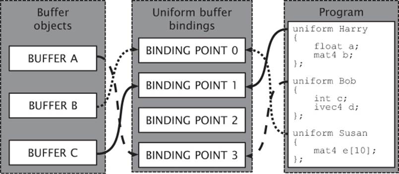
Figure 5.1: Binding buffers and uniform blocks to binding points
In Figure 5.1, there is a program with three uniform blocks (Harry, Bob, and Susan) and three buffer objects (A, B, and C). Harry is assigned to binding point 1, and buffer C is bound to binding point 1, so Harry’s data comes from buffer C. Likewise, Bob is assigned to binding point 3, to which buffer A is bound, and so Bob’s data comes from buffer A. Finally, Susan is assigned to binding point 0, and buffer B is bound to binding point 0, so Susan’s data comes from buffer B. Notice that binding point 2 is not used.
That doesn’t matter. There could be a buffer bound there, but the program doesn’t use it.
The code to set this up is simple and is given in Listing 5.18.
// Get the indices of the uniform blocks using glGetUniformBlockIndex
GLuint harry_index = glGetUniformBlockIndex(program, "Harry");
GLuint bob_index = glGetUniformBlockIndex(program, "Bob");
GLuint susan_index = glGetUniformBlockIndex(program, "Susan");
// Assign buffer bindings to uniform blocks, using their indices
glUniformBlockBinding(program, harry_index, 1);
glUniformBlockBinding(program, bob_index, 3);
glUniformBlockBinding(program, susan_index, 0);
// Bind buffers to the binding points
// Binding 0, buffer B, Susan's data
glBindBufferBase(GL_UNIFORM_BUFFER, 0, buffer_b);
// Binding 1, buffer C, Harry's data
glBindBufferBase(GL_UNIFORM_BUFFER, 1, buffer_c);
// Note that we skipped binding 2
// Binding 3, buffer A, Bob's data
glBindBufferBase(GL_UNIFORM_BUFFER, 3, buffer_a);
Listing 5.18: Specifying bindings for uniform blocks
Again, if we had set the bindings for our uniform blocks in our shader code by using the binding layout qualifier, we could avoid the calls to glUniformBlockBinding() in Listing 5.18. This example is shown in Listing 5.19.
layout (binding = 1) uniform Harry
{
// ...
};
layout (binding = 3) uniform Bob
{
// ...
};
layout (binding = 0) uniform Susan
{
// ...
};
Listing 5.19: Uniform blocks binding layout qualifiers
After a shader containing the declarations shown in Listing 5.19 is compiled and linked into a program object, the bindings for the Harry, Bob, and Susan uniform blocks will be set to the same things as they would be after executing Listing 5.18. Setting the uniform block binding in the shader can be useful for a number of reasons. First is that it reduces the number of calls to OpenGL that your application must make. Second, it allows the shader to associate a uniform block with a particular binding point without the application needing to know its name. This can be helpful if you have some data in a buffer with a standard layout, but want to refer to it with different names in different shaders.
A common use for uniform blocks is to separate steady state from transient state. By setting up the bindings for all your programs using a standard convention, you can leave buffers bound when you change the program. For example, if you have some relatively fixed state — say the projection matrix, the size of the viewport, and a few other things that change once a frame or less often — you can leave that information in a buffer bound to binding point zero. Then, if you set the binding for the fixed state to zero for all programs, whenever you switch program objects using glUseProgram(), the uniforms will be sitting there in the buffer, ready to use.
Now let’s say that you have a fragment shader that simulates some material (e.g., cloth or metal); you could put the parameters for the material into another buffer. In your program that shades that material, bind the uniform block containing the material parameters to binding point 1. Each object would maintain a buffer object containing the parameters of its surface. As you render each object, it uses the common material shader and simply binds its parameter buffer to buffer binding point 1.
A final significant advantage of uniform blocks is that they can be quite large. The maximum size of a uniform block can be determined by calling glGetIntegerv() and passing the GL_MAX_UNIFORM_BLOCK_SIZE parameter. Also, the number of uniform blocks that you can access from a single program can be retrieved by calling glGetIntegerv() and passing the GL_MAX_UNIFORM_BLOCK_BINDINGS. OpenGL guarantees that at least 64KB in size, and you can have at least 14 of them referenced by a single program. Taking the example of the previous paragraph a little further, you could pack all of the properties for all of the materials used by your application into a single, large uniform block containing a big array of structures. As you render the objects in your scene, you only need to communicate the index within that array of the material you wish to use. You can achieve that with a static vertex attribute or traditional uniform, for example. This could be substantially faster than replacing the contents of a buffer object or changing uniform buffer bindings between each object. If you’re really clever, you can even render objects made up from multiple surfaces with different materials using a single drawing command.
Using Uniforms to Transform Geometry
Back in Chapter 4, “Math for 3D Graphics,” you learned how to construct matrices that represent several common transformations including scale, translation, and rotation, and how to use the sb6::vmath library to do the heavy lifting for you. You also saw how to multiply matrices to produce a composite matrix that represents the whole transformation sequence. Given a point of interest and the camera’s location and orientation, you can build a matrix that will transform objects into the coordinate space of the viewer. Also, you can build matrices that represent perspective and orthographic projections onto the screen.
Furthermore, in this chapter you have seen how to feed a vertex shader with data from buffer objects, and how to pass data into your shaders through uniforms (whether in the default uniform block, or in a uniform buffer). Now it’s time to put all this together and build a program that does a little more than pass vertices through un-transformed.
Our example program will be the classic spinning cube. We’ll create geometry representing a unit cube located at the origin and store it in buffer objects. Then, we will use a vertex shader to apply a sequence of transforms to it to move it into world space. We will construct a basic view matrix, multiply our model and view matrices together to produce a model-view matrix, and create a perspective transformation matrix representing some of the properties of our camera. Finally, we will pass these into a simple vertex shader using uniforms and draw the cube on the screen.
First, let’s set up the cube geometry using a vertex array object. The code to do this is shown in Listing 5.20.
// First, create and bind a vertex array object
glGenVertexArrays(1, &vao);
glBindVertexArray(vao);
static const GLfloat vertex_positions[] =
{
-0.25f, 0.25f, -0.25f,
-0.25f, -0.25f, -0.25f,
0.25f, -0.25f, -0.25f,
0.25f, -0.25f, -0.25f,
0.25f, 0.25f, -0.25f,
-0.25f, 0.25f, -0.25f,
/* MORE DATA HERE */
-0.25f, 0.25f, -0.25f,
0.25f, 0.25f, -0.25f,
0.25f, 0.25f, 0.25f,
0.25f, 0.25f, 0.25f,
-0.25f, 0.25f, 0.25f,
-0.25f, 0.25f, -0.25f
};
// Now generate some data and put it in a buffer object
glGenBuffers(1, &buffer);
glBindBuffer(GL_ARRAY_BUFFER, buffer);
glBufferData(GL_ARRAY_BUFFER,
sizeof(vertex_positions),
vertex_positions,
GL_STATIC_DRAW);
// Set up our vertex attribute
glVertexAttribPointer(0, 3, GL_FLOAT, GL_FALSE, 0, NULL);
glEnableVertexAttribArray(0);
Listing 5.20: Setting up cube geometry
Next, on each frame, we need to calculate the position and orientation of our cube and calculate the matrix that represents them. We also build the camera matrix by simply translating in the z direction. Once we have built these matrices, we can multiply them together and pass them as uniforms into our vertex shader. The code to do this is shown in Listing 5.21.
float f = (float)currentTime * (float)M_PI * 0.1f;
vmath::mat4 mv_matrix =
vmath::translate(0.0f, 0.0f, -4.0f) *
vmath::translate(sinf(2.1f * f) * 0.5f,
cosf(1.7f * f) * 0.5f,
sinf(1.3f * f) * cosf(1.5f * f) * 2.0f) *
vmath::rotate((float)currentTime * 45.0f, 0.0f, 1.0f, 0.0f) *
vmath::rotate((float)currentTime * 81.0f, 1.0f, 0.0f, 0.0f);
Listing 5.21: Building the model-view matrix for a spinning cube
The projection matrix can be rebuilt whenever the window size changes. The sb6::application framework provides a function called onResize that handles resize events. If we override this function, then when the window size changes it will be called and we can projection matrix. We can load that into a uniform as well in our rendering loop. If the window size changes, we’ll also need to update our viewport with a call to glViewport(). Once we have put all our matrices into our uniforms, we can draw the cube geometry with the glDrawArrays() function. The code to update the projection matrix is shown in Listing 5.22 and the remainder of the rendering loop is shown in Listing 5.23.
void onResize(int w, int h)
{
sb6::application::onResize(w, h);
aspect = (float)info.windowWidth / (float)info.windowHeight;
proj_matrix = vmath::perspective(50.0f,
aspect,
0.1f,
1000.0f);
}
Listing 5.22: Updating the projection matrix for the spinning cube
// Clear the framebuffer with dark green
static const GLfloat green[] = { 0.0f, 0.25f, 0.0f, 1.0f };
glClearBufferfv(GL_COLOR, 0, green);
// Activate our program
glUseProgram(program);
// Set the model-view and projection matrices
glUniformMatrix4fv(mv_location, 1, GL_FALSE, mv_matrix);
glUniformMatrix4fv(proj_location, 1, GL_FALSE, proj_matrix);
// Draw 6 faces of 2 triangles of 3 vertices each = 36 vertices
glDrawArrays(GL_TRIANGLES, 0, 36);
Listing 5.23: Rendering loop for the spinning cube
Before we can actually render anything, we’ll need to write a simple vertex shader to transform the vertex positions using the matrices we’ve been given and to pass along the color information so that the cube isn’t just a flat blob. The vertex shader is shown in Listing 5.24 and the fragment shader is shown in Listing 5.25.
#version 430 core
in vec4 position;
out VS_OUT
{
vec4 color;
} vs_out;
uniform mat4 mv_matrix;
uniform mat4 proj_matrix;
void main(void)
{
gl_Position = proj_matrix * mv_matrix * position;
vs_out.color = position * 2.0 + vec4(0.5, 0.5, 0.5, 0.0);
}
Listing 5.24: Spinning cube vertex shader
#version 430 core
out vec4 color;
in VS_OUT
{
vec4 color;
} fs_in;
void main(void)
{
color = fs_in.color;
}
Listing 5.25: Spinning cube fragment shader
A few frames of the resulting application are shown in Figure 5.2.
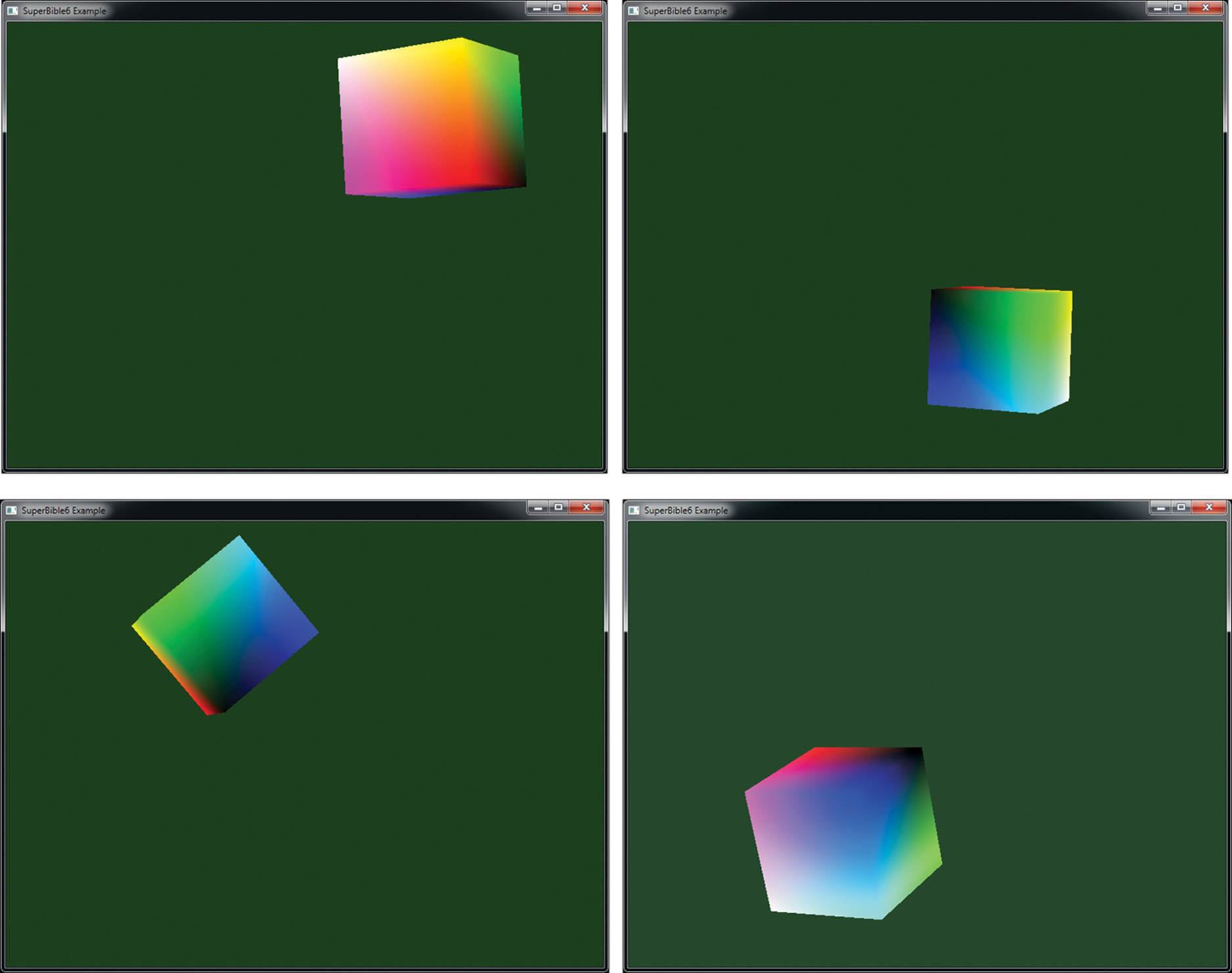
Figure 5.2: A few frames from the spinning cube application
Of course, now that we have our cube geometry in a buffer object and a model-view matrix in a uniform, there’s nothing to stop us from updating the uniform and drawing many copies of the cube in a single frame. In Listing 5.26 we’ve modified the rendering function to calculate a new model-view matrix many times and repeatedly draw our cube. Also, because we’re going to render many cubes in this example, we’ll need to clear the depth buffer before rendering the frame. Although not shown here, we also modified our startup function to enable depth testing and set the depth test function to GL_LEQUAL. The result of rendering with our modified program is shown in Figure 5.3.
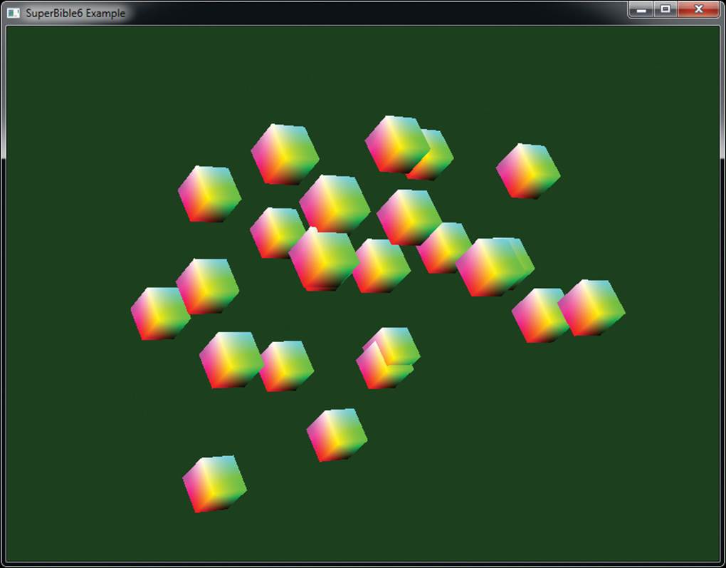
Figure 5.3: Many cubes!
// Clear the framebuffer with dark green and clear
// the depth buffer to 1.0
static const GLfloat green[] = { 0.0f, 0.25f, 0.0f, 1.0f };
static const GLfloat one = 1.0f;
glClearBufferfv(GL_COLOR, 0, green);
glClearBufferfv(GL_DEPTH, 0, &one);
// Activate our program
glUseProgram(program);
// Set the model-view and projection matrices
glUniformMatrix4fv(proj_location, 1, GL_FALSE, proj_matrix);
// Draw 24 cubes...
for (i = 0; i < 24; i++)
{
// Calculate a new model-view matrix for each one
float f = (float)i + (float)currentTime * 0.3f;
vmath::mat4 mv_matrix =
vmath::translate(0.0f, 0.0f, -20.0f) *
vmath::rotate((float)currentTime * 45.0f, 0.0f, 1.0f, 0.0f) *
vmath::rotate((float)currentTime * 21.0f, 1.0f, 0.0f, 0.0f) *
vmath::translate(sinf(2.1f * f) * 2.0f,
cosf(1.7f * f) * 2.0f,
sinf(1.3f * f) * cosf(1.5f * f) * 2.0f);
// Update the uniform
glUniformMatrix4fv(mv_location, 1, GL_FALSE, mv_matrix);
// Draw - notice that we haven't updated the projection matrix
glDrawArrays(GL_TRIANGLES, 0, 36);
}
Listing 5.26: Rendering loop for the spinning cube
Shader Storage Blocks
In addition to the read-only access to buffer objects that is provided by uniform blocks, buffer objects can also be used for general storage from shaders using shader storage blocks. These are declared in a similar manner to uniform blocks and backed in the same way by binding a range of buffer objects to one of the indexed GL_SHADER_STORAGE_BUFFER targets. However, the biggest difference between a uniform block and a shader storage block is that your shader can write into the shader storage block and, furthermore, it can even perform atomic operations on members of a shader storage block. Shader storage blocks also have a much higher upper size limit.
To declare a shader storage block, simply declare a block in the shader just like you would a uniform block, but rather than use the uniform keyword, use the buffer qualifier. Like uniform blocks, shader storage blocks support the std140 packing layout qualifier, but also support the std4303packing layout qualifier, which allows arrays of integers and floating-point variables (and structures containing them) to be tightly packed (something that is sorely lacking from std140). This allows better efficiency of memory use and tighter cohesion with structure layouts generated by compilers for languages such as C++. An example shader storage block declaration is shown in Listing 5.27.
3. The std140 and std430 packing layouts are named for the version of the shading language with which they were introduced — std140 with GLSL 1.40 (which was part of OpenGL 3.1), and std430 with GLSL 4.30, which was the version released with OpenGL 4.3.
#version 430 core
struct my_structure
{
int pea;
int carrot;
vec4 potato;
};
layout (binding = 0, std430) buffer my_storage_block
{
vec4 foo;
vec3 bar;
int baz[24];
my_structure veggies;
};
Listing 5.27: Example shader storage block declaration
The members of a shader storage block can be referred to just as any other variable. To read from them, you could, for example use them as a parameter to a function, and to write into them you simply assign to them. When the variable is used in an expression, the source of data will be the buffer object, and when the variable is assigned to, the data will be written into the buffer object. You can place data into the buffer using functions like glBufferData() just as you would with a uniform block. Because the buffer is writable by the shader, if you call glMapBuffer() withGL_READ_ONLY (or GL_READ_WRITE) as the access mode, you will be able read the data produced by your shader.
Shader storage blocks and their backing buffer objects provide additional advantages over uniform blocks. For example, their size is not really limited. Of course, if you go overboard, OpenGL may fail to allocate memory for you, but there really isn’t a hard-wired practical upper limit to the size of a shader storage block. Also, the newer packing rules for std430 allow an application’s data to be more efficiently packed and directly accessed than would a uniform block. It is worth noting, though, that due to the stricter alignment requirements of uniform blocks and smaller minimum size, some hardware may handle uniform blocks differently than shader storage blocks and execute more efficiently when reading from them. Listing 5.28 shows how you might use a shader storage block in place of regular inputs in a vertex shader.
#version 430 core
struct vertex
{
vec4 position;
vec3 color;
};
layout (binding = 0, std430) buffer my_vertices
{
vertex vertices[];
};
uniform mat4 transform_matrix;
out VS_OUT
{
vec3 color;
} vs_out;
void main(void)
{
gl_Position = transform_matrix * vertices[gl_VertexID].position;
vs_out.color = vertices[gl_VertexID].color;
}
Listing 5.28: Using a shader storage block in place of vertex attributes
Although it may seem that shader storage blocks offer so many advantages that they almost make uniform blocks and vertex attributes redundant, you should be aware that all of this additional flexibility makes it difficult for OpenGL to make access to storage blocks truly optimal. For example, some OpenGL implementations may be able to provide faster access to uniform blocks given the knowledge that their content will always be constant. Also, reading the input data for vertex attributes may happen long before your vertex shader runs, letting OpenGL’s memory subsystem keep up. Reading vertex data right in the middle of your shader might well slow it down quite a bit.
Atomic Memory Operations
In addition to simply reading and writing of memory, shader storage blocks allow you to perform atomic operations on memory. An atomic operation is a sequence of a read from memory potentially followed by a write to memory that must be uninterrupted for the result to be correct. Consider a case where two shader invocations perform the operation m = m + 1; using the same memory location represented by m. Each invocation will load the current value stored in the memory location represented by m, add one to it, and then write it back to memory at the same location.
If each invocation operates in lockstep, then we will end up with the wrong value in memory unless the operation can be made atomic. This is because the first invocation will load the value from memory, and then the second invocation will read the same value from memory. Both invocations will increment their copy of the value. The first invocation will write its incremented value back to memory, and then finally, the second invocation will overwrite that value with the same, incremented value that it calculated. This problem only gets worse when there are many more than two invocations running at a time.
To get around this problem, atomic operations cause the complete read-modify-write cycle to complete for one invocation before any other invocation gets a chance to even read from memory. In theory, if multiple shader invocations perform atomic operations on different memory locations, then everything should run nice and fast and work just as if you had written the naïve m = m + 1; code in your shader. If two invocations access the same memory locations (this is known as contention), then they will be serialized and only one will get to go at one time. To execute an atomic operation on a member of a shader storage block, you call one of the atomic memory functions listed in Table 5.4.
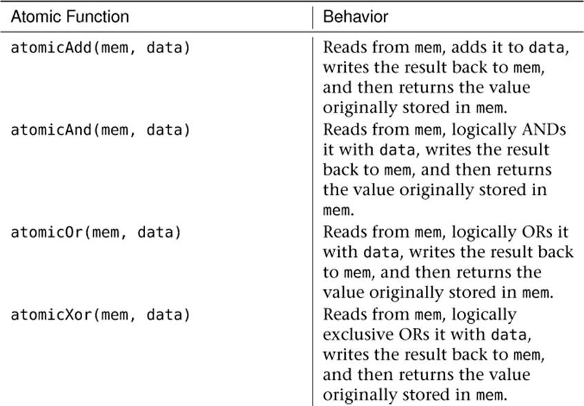
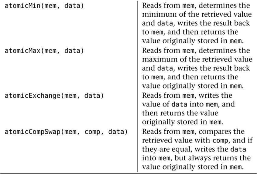
Table 5.4. Atomic Operations on Shader Storage Blocks
In Table 5.4, all of the functions have an integer (int) and unsigned integer (uint) version. For the integer versions, mem is declared as inout int mem, data and comp (for atomicCompSwap) are declared as int data, and int comp and the return value of all functions is int. Likewise, for the unsigned integer versions, all parameters are declared using uint and the return type of the function is uint. Notice that there are no atomic operations on floating-point variables, vectors, or matrices or integer values that are not 32 bits wide. All of the atomic memory access functions shown in Table 5.4 return the value that was in memory prior to the atomic operation taking place. When an atomic operation is attempted by multiple invocations of your shader to the same location at the same time, they are serialized, which means that they take turns. This means that you’re not guaranteed to receive any particular return value of an atomic memory operation.
Synchronizing Access to Memory
When you are only reading from a buffer, data is almost always going to be available when you think it should be and you don’t need to worry about the order in which your shaders read from it. However, when your shader starts writing data into buffer objects, either through writes to variables in shader storage blocks or through explicit calls to the atomic operation functions that might write to memory, there are cases where you need to avoid hazards.
Memory hazards fall roughly into three categories:
• A Read-After-Write (RAW) hazard can occur when your program attempts to read from a memory location right after it’s written to it. Depending on the system architecture, the read and write may be re-ordered such that the read actually ends up being executed before the write is complete, resulting in the old data being returned to the application.
• A Write-After-Write (WAW) hazard can occur when a program performs a write to the same memory location twice in a row. You might expect that whatever data was written last would overwrite the data written first and be the values that end up staying in memory. Again, on some architectures this is not guaranteed, and in some circumstances the first data written by the program might actually be the data that ends up in memory.
• Finally, a Write-After-Read (WAR) hazard normally only occurs in parallel processing systems (such as graphics processors) and may happen when one thread of execution (such as a shader invocation) performs a write to memory after another thread believes that it has written to memory. If these operations are re-ordered, the thread that performed the read may end up getting the data that was written by the second thread without expecting it.
Because of the deeply pipelined and highly parallel nature of the systems that OpenGL is expected to be running on, it includes a number of mechanisms to alleviate and control memory hazards. Without these features, OpenGL implementations would need to be far more conservative about reordering your shaders and running them in parallel. The main apparatus for dealing with memory hazards is the memory barrier.
A memory barrier essentially acts as a marker that tells OpenGL, “Hey, if you’re going to start reordering things, that’s fine — just don’t let anything I say after this point actually happen before anything I say before it.” You can insert barriers both in your application code with calls to OpenGL, and in your shaders.
Using Barriers in Your Application
The function to insert a barrier is glMemoryBarrier() and its prototype is
void glMemoryBarrier(GLbitfield barriers);
The glMemoryBarrier() function takes a GLbitfield parameter, barriers, which allows you to specify which of OpenGL’s memory subsystems should obey the barrier and which ones are free to ignore it and continue as they would have. The barrier affects ordering of memory operations in the categories specified in barriers. If you want to bash OpenGL with a big hammer and just synchronize everything, you can set barriers to GL_ALL_BARRIER_BITS. However, there are quite a number of bits defined that you can add together to be more precise about what you want to synchronize. A few examples are listed below:
• Including GL_SHADER_STORAGE_BARRIER_BIT tells OpenGL that you want it to let any accesses (writes in particular) performed by shaders that are run before the barrier complete before letting any shaders access the data after the barrier. This means that if you write into a shader storage buffer from a shader and then call glMemoryBarrier() with GL_SHADER_STORAGE_BARRIER_BIT included in barriers, shaders you run after the barrier will “see” that data. Without such a barrier, this is not guaranteed.
• Including GL_UNIFORM_BARRIER_BIT in barriers tells OpenGL that you might have written into memory that might be used as a uniform buffer after the barrier, and it should wait to make sure that shaders that write into the buffer have completed before letting shaders that use it as a uniform buffer run. You would set this, for example, if you wrote into a buffer using a shader storage block in a shader and then wanted to use that buffer as a uniform buffer later.
• Including GL_VERTEX_ATTRIB_ARRAY_BARRIER_BIT ensures that OpenGL will wait for shaders that write to buffers have completed before using any of those buffers as the source of vertex data through a vertex attribute. For example, you would set this if you write into a buffer through a shader storage block and then want to use that buffer as part of a vertex array to feed data into the vertex shader of a subsequent drawing command.
There are plenty more of these bits that control the ordering of shaders with respect to OpenGL’s other subsystems, and we will introduce them as we talk more in depth about those subsystems. The key to remember about glMemoryBarrier() is that the items included in barriers are thedestination subsystems and that the mechanism by which you updated the data isn’t relevant.
Using Barriers in Your Shaders
Just as you can insert memory barriers in your application’s code to control the ordering of memory accesses performed by your shaders relative to your application, you can also insert barriers into your shaders to stop OpenGL from reading or writing memory in some order other than what your shader code says. The basic memory barrier function in GLSL is
void memoryBarrier();
If you call memoryBarrier() from your shader code, any memory reads or writes that you might have performed will complete before the function returns. This means that it’s safe to go read data back that you might have just written. Without a barrier, it’s even possible that when you read from a memory location that you just wrote to that OpenGL will return old data to you instead of the new!
To provide finer control over what types of memory accesses are ordered, there are some more specialized versions of the memoryBarrier(). For example, memoryBarrierBuffer() orders only transactions on reads and writes to buffers, but to nothing else. We’ll introduce the other barrier functions as we talk about the types of data that they protect.
Atomic Counters
Atomic counters are a special type of variable that represents storage that is shared across multiple shader invocations. This storage is backed by a buffer object, and functions are provided in GLSL to increment and decrement the values stored in the buffer. What is special about these operations is that they are atomic, and just as with the equivalent functions for members of shader storage blocks (shown in Table 5.4), they return the original value of the counter before it was modified. Just like the other atomic operations, if two shader invocations increment the same counter at the same time, OpenGL will make them take turns. One shader invocation will receive the original value of the counter, the other will receive the original value plus one, and the final value of the counter will be that of the original value plus two. Also, just as with shader storage block atomics, it should be noted that there is no guarantee of the order that these operations will occur, and so you can’t rely on receiving any specific value.
To declare an atomic counter in a shader, do this:
layout (binding = 0) uniform atomic_uint my_variable;
OpenGL provides a number of binding points to which you can bind the buffers where it will store the values of atomic counters. Additionally, each atomic counter is stored at a specific offset within the buffer object. The buffer binding index and the offset within the buffer bound to that binding can be specified using the binding and offset layout qualifiers that can be applied to an atomic counter uniform declaration. For example, if we wish to place my_variable at offset 8 within the buffer bound to the buffer bound to atomic counter binding point 3, then we could write
layout (binding = 3, offset = 8) uniform atomic_uint my_variable;
In order to provide storage for the atomic counter, we can now bind a buffer object to the GL_ATOMIC_COUNTER_BUFFER indexed binding point. Listing 5.29 shows how to do this.
// Generate a buffer name
GLuint buf;
glGenBuffers(1, &buf);
// Bind it to the generic GL_ATOMIC_COUNTER_BUFFER target and
// initialize its storage
glBindBuffer(GL_ATOMIC_COUNTER_BUFFER, buf);
glBufferData(GL_ATOMIC_COUNTER_BUFFER, 16 * sizeof(GLuint),
NULL, GL_DYNAMIC_COPY);
// Now bind it to the fourth indexed atomic counter buffer target
glBindBufferBase(GL_ATOMIC_COUNTER_BUFFER, 3, buf);
Listing 5.29: Setting up an atomic counter buffer
Before using the atomic counter in your shader, it’s a good idea to reset it first. To do this, you can either call glBufferSubData() and pass the address of a variable holding the value you want to reset the counter(s) to, map the buffer using glMapBufferRange(), and write the values directly into it, or use glClearBufferSubData(). Listing 5.30 shows an example of all three methods.
// Bind our buffer to the generic atomic counter buffer
// binding point
glBindBuffer(GL_ATOMIC_COUNTER_BUFFER, buf);
// Method 1 - use glBufferSubData to reset an atomic counter.
const GLuint zero = 0;
glBufferSubData(GL_ATOMIC_COUNTER_BUFFER, 2 * sizeof(GLuint),
sizeof(GLuint), &zero);
// Method 2 - Map the buffer and write the value directly into it
GLuint * data =
(GLuint *)glMapBufferRange(GL_ATOMIC_COUNTER_BUFFER,
0, 16 * sizeof(GLuint),
GL_MAP_WRITE_BIT |
GL_MAP_INVALIDATE_RANGE_BIT);
data[2] = 0;
glUnmapBuffer(GL_ATOMIC_COUNTER_BUFFER);
// Method 3 - use glClearBufferSubData
glClearBufferSubData(GL_ATOMIC_COUNTER_BUFFER,
GL_R32UI,
2 * sizeof(GLuint),
sizeof(GLuint),
GL_RED_INTEGER, GL_UNSIGNED_INT,
&zero);
Listing 5.30: Setting up an atomic counter buffer
Now that you have created a buffer and bound it to an atomic counter buffer target, and you declared an atomic counter uniform in your shader, you are ready to start counting things. First, to increment an atomic counter, call
uint atomicCounterIncrement(atomic_uint c);
This function reads the current value of the atomic counter, adds one to it, writes the new value back to the atomic counter, and returns the original value it read, and it does it all atomically. Because the order of execution between different invocations of your shader is not defined, callingatomicCounterIncrement twice in a row won’t necessarily give you two consecutive values. To decrement an atomic counter, call
uint atomicCounterDecrement(atomic_uint c);
This function reads the current value of the atomic counter, subtracts one from it, writes the value back into the atomic counter and returns the new value of the counter to you. Notice that this is the opposite of atomicCounterIncrement. If only one invocation of a shader is executing, and it calls atomicCounterIncrement followed by atomicCounterDecrement, it should receive the same value from both functions. However, in most cases, many invocations of the shader will be executing in parallel, and in practice, it is unlikely that you will receive the same value from a pair of calls to these functions. If you simply want to know the value of an atomic counter, you can call
uint atomicCounter(atomic_uint c);
This function simply returns the current value stored in the atomic counter c. As an example of using atomic counters, Listing 5.31 shows a simple fragment shader that increments an atomic counter each time it executes. This has the effect of producing the screen space area of the objects rendered with this shader in the atomic counter.
#version 430 core
layout (binding = 0, offset = 0) uniform atomic_uint area;
void main(void)
{
atomicCounterIncrement(area);
}
Listing 5.31: Counting area using an atomic counter
One thing you might notice about the shader in Listing 5.31 is that it doesn’t have any regular outputs (variables declared with the out storage qualifier) and won’t write any data into the framebuffer. In fact, we’ll disable writing to the framebuffer while we run this shader. To turn off writing to the framebuffer, we can call
glColorMask(GL_FALSE, GL_FALSE, GL_FALSE, GL_FALSE);
To turn framebuffer writes back on again, we can call
glColorMask(GL_TRUE, GL_TRUE, GL_TRUE, GL_TRUE);
Because atomic counters are stored in buffers, it’s possible now to bind our atomic counter to another buffer target, such as one of the GL_UNIFORM_BUFFER targets, and retrieve its value in a shader. This allows us to use the value of an atomic counter to control the execution of shaders that your program runs later. Listing 5.32 shows an example shader that reads the result of our atomic counter through a uniform block and uses it as part of the calculation of its output color.
#version 430 core
layout (binding = 0) uniform area_block
{
uint counter_value;
};
out vec4 color;
uniform float max_area;
void main(void)
{
float brightness = clamp(float(counter_value) / max_area,
0.0, 1.0);
color = vec4(brightness, brightness, brightness, 1.0);
}
Listing 5.32: Using the result of an atomic counter in a uniform block
When we execute the shader in Listing 5.31, it simply counts the area of the geometry that’s being rendered. That area then shows up in Listing 5.32 as the first and only member of the area_block uniform buffer block. We divide it by the maximum expected area and then use that as the brightness of further geometry. Consider what happens when we render with these two shaders. If an object is close to the viewer, it will appear larger and cover more screen area — the ultimate value of the atomic counter will be greater. When the object is far from the viewer, it will be smaller and the atomic counter won’t reach such a high value. The value of the atomic counter will be reflected in the uniform block in the second shader, affecting the brightness of the geometry it renders.
Synchronizing Access to Atomic Counters
Atomic counters represent locations in buffer objects. While shaders are executing, their values may well reside in special memory inside the graphics processor (which is what makes them faster than simple atomic memory operations on members of shader storage blocks, for example). However, when your shader is done executing, the values of the atomic counters will be written back into memory. As such, incrementing and decrementing atomic counters is considered a form of memory operation and so can be susceptible to the hazards described earlier in this chapter. In fact, the glMemoryBarrier() function supports a bit specifically for synchronizing access to atomic counters with other parts of the OpenGL pipeline. Calling
glMemoryBarrier(GL_ATOMIC_COUNTER_BARRIER_BIT);
will ensure that any access to an atomic counter in a buffer object will reflect updates to that buffer by a shader. You should call glMemoryBarrier() with the GL_ATOMIC_COUNTER_BARRIER_BIT set when something has written to a buffer that you want to see reflected in the values of your atomic counters. If you update the values in a buffer using an atomic counter and then use that buffer for something else, the bit you include in the barriers parameter to glMemoryBarrier() should correspond to what you want that buffer to be used for, which will not necessarily includeGL_ATOMIC_COUNTER_BARRIER_BIT.
Similarly, there is a version of the GLSL memoryBarrier() function, memoryBarrierAtomicCounter(), that ensures that operations on atomic counters are completed before it returns.
Textures
Textures are a structured form of storage that can be made accessible to shaders both for reading and writing. They are most often used to store image data and come in many forms. Perhaps the most common texture layout is two dimensional, but textures can also be created in one-dimensional or three-dimensional layouts, array forms (with multiple textures stacked together to form one logical object), cubes, and so on. Textures are represented as objects that can be generated, bound to texture units, and manipulated. To create a texture, first we need to ask OpenGL to reserve a name for us by calling glGenTextures(). At this point, the name we get back represents a yet-to-be-created texture object, and it only begins its life as a texture once it’s been bound to a texture target. This is similar to binding a buffer object to one of the buffer binding points. However, once you bind a texture name to a texture target, it takes the type of that target until it is destroyed.
Creating and Initializing Textures
The full creation of a texture involves generating a name and binding it to one of the texture targets, and then telling OpenGL what size image you want to store in it. Listing 5.33 shows how to generate a name for a texture object using glGenTextures(), use glBindTexture() to bind it to theGL_TEXTURE_2D target (which is one of several available texture targets), and then use the glTexStorage2D() function to allocate storage for the texture.
// The type used for names in OpenGL is GLuint
GLuint texture;
// Generate a name for the texture
glGenTextures(1, &texture);
// Now bind it to the context using the GL_TEXTURE_2D binding point
glBindTexture(GL_TEXTURE_2D, texture);
// Specify the amount of storage we want to use for the texture
glTexStorage2D(GL_TEXTURE_2D, // 2D texture
1, // 1 mipmap level
GL_RGBA32F, // 32-bit floating-point RGBA data
256, 256); // 256 × 256 texels
Listing 5.33: Generating, binding, and initializing a texture
Compare Listing 5.33 and Listing 5.1 and note how similar they are. In both cases, you reserve a name for an object, bind it to a target, and then define the storage for the data they contain. For textures, the function we’ve used to do this is glTexStorage2D(). It takes as parameters the target for the operation, which is the one we used to bind the texture; the number of levels that are used in mipmapping, which we are not using here (but will explain shortly); the internal format of the texture (we chose GL_RGBA32F here, which is a four-channel floating-point format); and the width and height of the texture. When we call this function, OpenGL will allocate enough memory to store a texture with those dimensions for us. Next, we need to specify some data for the texture. To do this, we use glTexSubImage2D() as shown in Listing 5.34.
// Define some data to upload into the texture
float * data = new float[256 * 256 * 4];
// generate_texture() is a function that fills memory with image data
generate_texture(data, 256, 256);
// Assume the texture is already bound to the GL_TEXTURE_2D target
glTexSubImage2D(GL_TEXTURE_2D, // 2D texture
0, // Level 0
0, 0, // Offset 0, 0
256, 256, // 256 × 256 texels, replace entire image
GL_RGBA, // Four channel data
GL_FLOAT, // Floating-point data
data); // Pointer to data
// Free the memory we allocated before - OpenGL now has our data
delete [] data;
Listing 5.34: Updating texture data with glTexSubImage2D()
Texture Targets and Types
The example in Listing 5.34 demonstrates how to create a 2D texture by binding a new name to the 2D texture target specified with GL_TEXTURE_2D. This is just one of several targets that are available to bind textures to, and a new texture object takes on the type determined by the target to which it is first bound. Thus, texture targets and types are often used interchangeably. Table 5.5 lists the available targets and describes the type of texture that will be created when a new name is bound to that target.
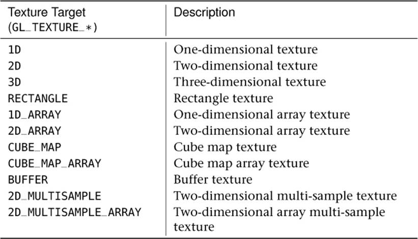
Table 5.5. Texture Targets and Description
The GL_TEXTURE_2D texture target is probably the one you will deal with the most. This is our standard, two-dimensional image that you imagine could be wrapped around objects. The GL_TEXTURE_1D and GL_TEXTURE_3D types allow you to create one-dimensional and three-dimensional textures, respectively. A 1D texture behaves just like a 2D texture with a height of 1, for the most part. A 3D texture, on the other hand, can be used to represent a volume and actually has a three-dimensional texture coordinate. The rectangle texture4 is a special case of 2D textures that have subtle differences in how they are read in shaders and which parameters they support.
4. Rectangle textures were introduced into OpenGL when not all hardware could support textures whose dimensions were not integer powers of two. Modern graphics hardware supports this almost universally, and so rectangle textures have essentially become a subset of the 2D texture and there isn’t much need to use one in preference to a 2D texture.
The GL_TEXTURE_1D_ARRAY and GL_TEXTURE_2D_ARRAY types represent arrays of texture images aggregated into single object. They are covered in more detail later in this chapter. Likewise, cube map textures (created by binding a texture name to the GL_TEXTURE_CUBE_MAP target) represent a collection of six square images that form a cube, which can be used to simulate lighting environments, for example. Just as the GL_TEXTURE_1D_ARRAY and GL_TEXTURE_2D_ARRAY represent 1D and 2D textures that are arrays of 1D or 2D images, the GL_TEXTURE_CUBE_MAP_ARRAY target represents a texture that is an array of cube maps.
Buffer textures, represented by the GL_TEXTURE_BUFFER target, are a special type of texture that are much like a 1D texture, except that their storage is actually represented by a buffer object. Besides this, they differ from a 1D texture in that their maximum size can be much larger than a 1D texture. The minimum requirement from the OpenGL specification is 65536 texels, but in practice most implementations will allow you to create much larger buffers — usually in the range of several hundred megabytes. Buffer textures also lack a few of the features supported by the 1D texture type such as filtering and mipmaps.
Finally, the multi-sample texture types GL_TEXTURE_2D_MULTISAMPLE and GL_TEXTURE_2D_MULTISAMPLE_ARRAY are used for multi-sample antialiasing, which is a technique for improving image quality, especially at the edges of lines and polygons.
Reading from Textures in Shaders
Once you’ve created a texture object and placed some data in it, you can read that data in your shaders and use it to color fragments, for example. Textures are represented in shaders as sampler variables and are hooked up to the outside world by declaring uniforms with sampler types. Just as there can be textures with various dimensionalities and that can be created and used through the various texture targets, there are corresponding sampler variable types that can be used in GLSL to represent them. The sampler type that represents two-dimensional textures is sampler2D. To access our texture in a shader, we can create a uniform variable with the sampler2D type, and then use the texelFetch built-in function with that uniform and a set of texture coordinates at which to read from the texture. Listing 5.35 shows an example of how to read from a texture in GLSL.
#version 430 core
uniform sampler2D s;
out vec4 color;
void main(void)
{
color = texelFetch(s, ivec2(gl_FragCoord.xy), 0);
}
Listing 5.35: Reading from a texture in GLSL
The shader of Listing 5.35 simply reads from the uniform sampler s using a texture coordinate derived from the built-in variable gl_FragCoord. This variable is an input to the fragment shader that holds the floating-point coordinate of the fragment being processed in window coordinates. However, the texelFetch function accepts integer-point coordinates that range from (0, 0) to the width and height of the texture. Therefore, we construct a two-component integer vector (ivec2) from the x and y components of gl_FragCoord. The third parameter to texelFetch is the mipmap level of the texture. Because the texture in this example has only one level, we set this to zero. The result of using this shader with our single-triangle example is shown in Figure 5.4.
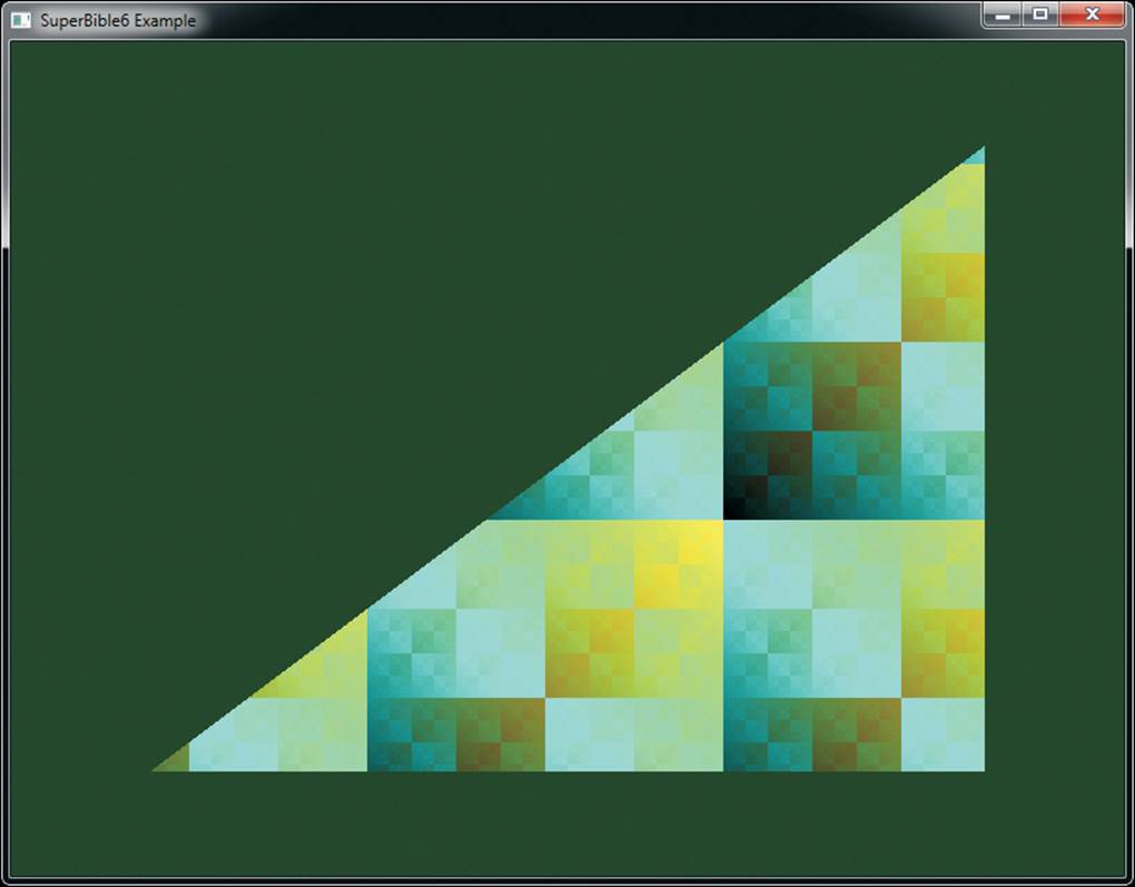
Figure 5.4: A simple textured triangle
Sampler Types
Each dimensionality of texture has a target to which texture objects are bound, which were introduced in the previous section, and each target has a corresponding sampler type that is used in your shader to access them. Table 5.6 lists the basic texture types and the sampler that should be used in shaders to access them.
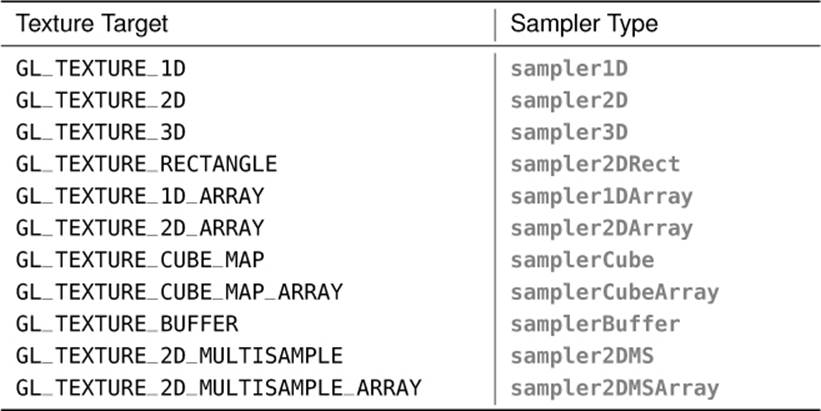
Table 5.6. Basic Texture Targets and Sampler Types
You should be able to see from the table that to create a 1D texture and then use it in your shader, you would bind a new texture name to the GL_TEXTURE_1D target and then use a sampler1D variable in your shader to read from it. Likewise, for 2D textures, you’d use GL_TEXTURE_2D andsampler2D, and for 3D textures, you’d use GL_TEXTURE_3D and sampler3D, and so on.
The GLSL sampler types sampler1D, sampler2D, and so on represent floating-point data. It is also possible to store signed and unsigned integer data in textures and retrieve that in your shader. To represent a texture containing signed integer data, we prefix the equivalent floating-point sampler type with i. Similarly, to represent a texture containing unsigned integer data, we prefix the equivalent floating-point sampler type with u. For example, a 2D texture containing signed integer data would be represented by a variable of type isampler2D, and a 2D texture containing unsigned integer data would be represented by a variable of type usampler2D.
As shown in our introductory example of Listing 5.35, we read from textures in shaders using the texelFetch built-in function. There are actually many variations of this function as it is overloaded. This means that there are several versions of the function that each have a different set of function parameters. Each function takes a sampler variable as the first parameter, with the main differentiator between the functions being the type of that sampler. The remaining parameters to the function depend on the type of sampler being used. In particular, the number of components in the texture coordinate depend on the dimensionality of the sampler, and the return type of the function depends on the type of the sampler (floating point, signed integer, or unsigned integer). For example, the following are all declarations of the texelFetch function:
vec4 texelFetch(sampler1D s, int P, int lod);
vec4 texelFetch(sampler2D s, ivec2 P, int lod);
ivec4 texelFetch(isampler2D s, ivec2 P, int lod);
uvec4 texelFetch(usampler3D s, ivec3 P, int lod);
Notice how the version of texelFetch that takes a sampler1D sampler type expects a one-dimensional texture coordinate, int P, but the version that takes a sampler2D expects a two-dimensional coordinate, ivec2 P. You can also see that the return type of the texelFetch function is influenced by the type of sampler that it takes. The version of texelFetch that takes a sampler2D produces a floating-point vector, whereas the version that takes a isampler2D sampler returns an integer vector. This type of overloading is similar to that supported by languages such as C++. That is, functions can be overloaded by parameter types, but not by return type, unless that return type is determined by one of the parameters.
All of the texture functions return a four-component vector, regardless of whether that vector is floating point or integer, and independently from the format of the texture object bound to the texture unit referenced by the sampler variable. If you read from a texture that contains fewer than four channels, the default value of zero will be filled in for the green and blue channels and one for the alpha channel. If one or more channels of the returned data never gets used by your shader, that’s fine, and it is likely that the shader compiler will optimize away any code that becomes redundant as a result.
Loading Textures from Files
In our simple example, we generated the texture data directly in our application. However, this clearly isn’t practical in a real-world application where you most likely have images stored on disk or on the other end of a network connection. Your options are either to convert your textures into hard-coded arrays (yes, there are utilities that will do this for you) or to load them from files within your application.
There are lots of image file formats that store pictures with or without compression, some of which are more suited to photographs and some more suited to line drawings or text. However, very few image formats exist that can properly store all of the formats supported by OpenGL or represent advanced features such as mipmaps, cubemaps, and so on. One such format is the .KTX format, or the Khronos TeXture format, which was specifically designed for the storage of pretty much anything that can be represented as an OpenGL texture. In fact, the .KTX file format includes most of the parameters you need to pass to texturing functions such as glTexStorage2D() and glTexSubImage2D() in order to load the texture directly in the file.
The structure of a .KTX file header is shown in Listing 5.36.
struct header
{
unsigned char identifier[12];
unsigned int endianness;
unsigned int gltype;
unsigned int gltypesize;
unsigned int glformat;
unsigned int glinternalformat;
unsigned int glbaseinternalformat;
unsigned int pixelwidth;
unsigned int pixelheight;
unsigned int pixeldepth;
unsigned int arrayelements;
unsigned int faces;
unsigned int miplevels;
unsigned int keypairbytes;
};
Listing 5.36: The header of a .KTX file
In this header, identifier contains a series of bytes that allow the application to verify that this is a legal .KTX file and endianness contains a known value that will be different depending on whether a little-endian or big-endian machine created the file. The gltype, glformat, glinternalformat, and glbaseinternalformat fields are actually the raw values of the GLenum types that will be used to load the texture. The gltypesize field stores the size, in bytes, of one element of data in the gltype type, and is used in case the endianness of the file does not match the native endianness of the machine loading the file, in which case, each element of the texture must be byte-swapped as it is loaded. The remaining fields, pixelwidth, pixelheight, pixeldepth, arrayelements, faces, and miplevels, store information about the dimensions of the texture. Finally, the keypairbytes field is used to allow applications to store additional information after the header and before the texture data. After this information, the raw texture data begins.
Because the .KTX file format was designed specifically for use in OpenGL-based applications, writing the code to load .KTX file is actually pretty straightforward. Even so, a basic loader for .KTX files is included in this book’s source code. To use the loader, you can simply reserve a new name for a texture using glGenTextures(), and then pass it, along with the filename of the .KTX file, to the loader. If you wish, you can even omit the OpenGL name for the texture (or pass zero) and the loader will call glGenTextures() for you. If the .KTX file is recognized, the loader will bind the texture to the appropriate target and load it with the data from the .KTX file. An example is shown in Listing 5.37.
// Generate a name for the texture
glGenTextures(1, &texture);
// Load texture from file
sb6::ktx::file::load("media/textures/icemoon.ktx", texture);
Listing 5.37: Loading a .KTX file
If you think that Listing 5.37 looks simple... you’d be right. The .KTX loader takes care of almost all the details for you. If the loader was successful in loading and allocating the texture, it will return the name of the texture you passed in (or the one it generated for you), and if it fails for some reason, it will return zero. After the loader returns, it leaves the texture bound to the texture unit that was active when it was called. That means that you can call glActiveTexture(), then call sb6::ktx::file::load, and the texture will be left bound to your selected texture unit. Don’t forget to delete the texture when you’re done with it by calling glDeleteTextures() on the name returned by the .KTX loader. Applying the texture loaded in the example above to the whole viewport produces the image shown in Figure 5.5.
Figure 5.5: A full-screen texture loaded from a .KTX file
Texture Coordinates
In the simple example shown earlier in this chapter, we simply used the current fragment’s window-space coordinate as the position at which to read from the texture. However, you can use any value you want, but in a fragment shader, they will usually be derived from one of the inputs that are smoothly interpolated from across each primitive by OpenGL. It is then the vertex (or geometry or tessellation evaluation) shader’s responsibility to produce the values of these coordinates. The vertex shader will generally pull the texture coordinates from a per-vertex input and pass them through unmodified. When you use multiple textures in your fragment shader, there is nothing to stop you from using a unique set of texture coordinates for each texture, but for most applications, a single set of texture coordinates would be used for every texture.
A simple vertex shader that accepts a single texture coordinate and passes it through to the fragment shader is shown in Listing 5.38 with the corresponding fragment shader shown in Listing 5.39.
#version 430 core
uniform mat4 mv_matrix;
uniform mat4 proj_matrix;
layout (location = 0) in vec4 position;
layout (location = 4) in vec2 tc;
out VS_OUT
{
vec2 tc;
} vs_out;
void main(void)
{
// Calculate the position of each vertex
vec4 pos_vs = mv_matrix * position;
// Pass the texture coordinate through unmodified
vs_out.tc = tc;
gl_Position = proj_matrix * pos_vs;
}
Listing 5.38: Vertex shader with single texture coordinate
The shader shown in Listing 5.39 not only takes as input the texture coordinate produced by the vertex shader, but also scales it non-uniformly. The textures wrapping modes are set to GL_REPEAT, which means that the texture will be repeated several times across the object.
#version 430 core
layout (binding = 0) uniform sampler2D tex_object;
// Input from vertex shader
in VS_OUT
{
vec2 tc;
} fs_in;
// Output to framebuffer
out vec4 color;
void main(void)
{
// Simply read from the texture at the (scaled) coordinates, and
// assign the result to the shader's output.
color = texture(tex_object, fs_in.tc * vec2(3.0, 1.0));
}
Listing 5.39: Fragment shader with single texture coordinate
By passing a texture coordinate with each vertex, we can wrap a texture around an object. Texture coordinates can then be generated offline procedurally or assigned by hand by an artist using a modeling program and stored in an object file. If we load a simple checkerboard pattern into a texture and apply it to an object, we can see how the texture is wrapped around it. Such an example is shown in Figure 5.6. On the left is the object with a checkerboard pattern wrapped around it. On the right is the same object using a texture loaded from a file.
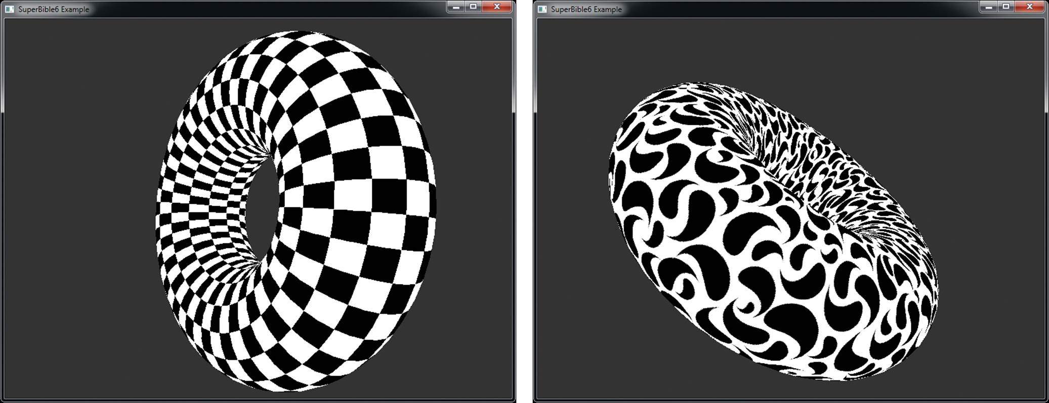
Figure 5.6: An object wrapped in simple textures
Controlling How Texture Data Is Read
OpenGL provides a lot of flexibility in how it reads data from textures and returns it to your shader. Usually, texture coordinates are normalized — that is, they range between 0.0 and 1.0. OpenGL lets you control what happens when the texture coordinates you supply fall outside this range. This is called the wrapping mode of the sampler. Also, you get to decide how values between the real samples are calculated. This is called the filtering mode of a sampler. The parameters controlling the wrapping and filtering mode of a sampler are stored in a sampler object.
To create one or more sampler objects, call
void glGenSamplers(GLsizei n, GLuint * samplers);
Here, n is the number of sampler objects you want to create, and samplers is the address of at least n unsigned integer variables that will be used to store the names of the newly created sampler objects.
Sampler objects are manipulated slightly differently than other objects in OpenGL. The two main functions you will use to set the parameters of a sampler object are
void glSamplerParameteri(GLuint sampler,
GLenum pname,
GLint param);
and
void glSamplerParameterf(GLuint sampler,
GLenum pname,
GLfloat param);
Notice that glSamplerParameteri() and glSamplerParameterf() both take the sampler object name as the first parameter. This means that you can directly modify a sampler object without binding it to a target first. You will need to bind a sampler object to use it, but in this case, you bind it to a texture unit just as you would a texture. The function used to bind a sampler object to one of the texture units is glBindSampler(), whose prototype is
void glBindSampler(GLuint unit, GLuint sampler);
For glBindSampler(), rather than taking a texture target, it takes the index of the texture unit to which to bind the sampler object. Together, the sampler object and texture object bound to a given texture unit form a complete set of data and parameters required for constructing texels as demanded by your shaders. By separating the parameters of the texture sampler from the texture data, this provides three important behaviors:
• It allows you to use the same set of sampling parameters for a large number of textures without needing to specify those parameters for each of the textures.
• It allows you to change the texture bound to a texture unit without updating the sampler parameters.
• It allows you to read from the same texture with multiple sets of sampler parameters at the same time.
Although non-trivial applications will likely opt to use their own sampler objects, each texture effectively contains an embedded sampler object that contains the sampling parameters to be used for that texture when no sampler object is bound to the corresponding texture unit. You can think of this as the default sampling parameters for a texture. To access the sampler object stored inside a texture object, you need to bind it to its target and then call
void glTexParameterf(GLenum target,
GLenum pname,
GLfloat param);
or
void glTexParameteri(GLenum target,
GLenum pname,
GLint param);
In these cases, the target parameter specifies the target to which the texture you want to access is bound, and pname and param have the same meanings as for glSamplerParameteri() and glSamplerParameterf().
Using Multiple Textures
If you want to use multiple textures in a single shader, you will need to create multiple sampler uniforms and set them up to reference different texture units. You’ll also need to bind multiple textures to your context at the same time. To allow this, OpenGL supports multiple texture units. The number of units supported can be queried by calling glGetIntegerv() with the GL_MAX_COMBINED_TEXTURE_IMAGE_UNITS parameter, as in
GLint units;
glGetIntegerv(GL_MAX_COMBINED_TEXTURE_IMAGE_UNITS, &units);
This will tell you the maximum number of texture units that might be accessible to all shader stages at any one time. To bind a texture to a specific texture unit, you first need to change the active texture unit selector, by calling glActiveTexture() with a texture unit identifier. This identifier is the value of the token GL_TEXTURE0 plus the index of the texture unit you want to select. For example, to select texture unit 5, call
glActiveTexture(GL_TEXTURE0 + 5);
For your convenience, the standard OpenGL header files define the tokens GL_TEXTURE1 through GL_TEXTURE31 as the values of GL_TEXTURE0 plus the values 1 through 31. Given this, to bind three textures to your context, you could use code such as
GLuint textures[3];
glGenTextures(3, &textures);
glActiveTexture(GL_TEXTURE0);
glBindTexture(GL_TEXTURE_2D, textures[0]);
glActiveTexture(GL_TEXTURE1);
glBindTexture(GL_TEXTURE_2D, textures[1]);
glActiveTexture(GL_TEXTURE2);
glBindTexture(GL_TEXTURE_2D, textures[2]);
Once you have bound multiple textures to your context, you need to make the sampler uniforms in your shaders refer to the different units. There are two ways to do this; the first is to use the glUniform1i() function to set the value of the sampler uniform directly from your application’s code. Because samplers are declared as uniforms in your shader code, you can call glGetUniformLocation() to find their location and then modify their value. Sampler variables don’t have a value that can actually be read as an integer in shaders, but for the purposes of setting the texture unit to which it refers, it is treated as an integer uniform and hence the use of the glUniform1i() function. The second way to set the texture unit referred to by a sampler uniform is to initialize its value at shader compilation time by using the binding layout qualifier in your shader code. To create three sampler uniforms referring to texture units 0, 1, and 2, we can write
layout (binding = 0) uniform sampler2D foo;
layout (binding = 1) uniform sampler2D bar;
layout (binding = 2) uniform sampler2D baz;
After compiling this code and linking it into a program object, the sampler foo will reference texture unit 0, bar will reference unit 1, and baz will reference unit 2. The unit to which the sampler uniform refers can still be changed after the program has been linked by calling the glUniform1i()function. However, setting the unit directly in the shader code is far more convenient and does not require changes to the application’s source code. This is the method we will use in the majority of the samples in the remainder of the book.
Texture Filtering
There is almost never a one-to-one correspondence between texels in the texture map and pixels on the screen. A careful programmer could achieve this result, but only by texturing geometry that was carefully planned to appear on-screen such that the texels and pixels lined up. (This is actually often done when OpenGL is used for image processing applications.) Consequently, texture images are always either stretched or shrunk as they are applied to geometric surfaces. Due to the orientation of the geometry, a given texture could even be stretched and shrunk at the same time across the surface of some object.
In the samples presented so far, we have been using the texelFetch() function, which fetches a single texel from the selected texture at specific integer texture coordinates. Clearly, to achieve a fragment-to-texel ratio that is not an integer, this function isn’t going to cut it. Here, we need a more flexible function, and that function is simply called texture(). Like texelFetch(), it has several overloaded prototypes:
vec4 texture(sampler1D s, float P);
vec4 texture(sampler2D s, vec2 P);
ivec4 texture(isampler2D s, vec2 P);
uvec4 texture(usampler3D s, vec3 P);
As you might have noticed, unlike the texelFetch() function, the texture() function accepts floating-point texture coordinates. The range 0.0 to 1.0 in each dimension maps exactly once onto the texture. However, the texture coordinates can have any value in between, and can even stray far outside the range 0.0 to 1.0. The next few sections describe how OpenGL takes these floating-point numbers and uses them to produce texel values for your shaders.
The process of calculating color fragments from a stretched or shrunken texture map is called texture filtering. Stretching a texture is also known as magnification, and shrinking a texture is also known as minification. Using the sampler parameter functions, OpenGL allows you to set both magnification and minification filters. The parameter names for these two filters are GL_TEXTURE_MAG_FILTER and GL_TEXTURE_MIN_FILTER. For now, you can select from two basic texture filters for them, GL_NEAREST and GL_LINEAR, which correspond to nearest neighbor and linear filtering. Make sure you always choose one of these two filters for the GL_TEXTURE_MIN_FILTER — the default filter setting does not work without mipmaps (see the next section “Mipmaps”).
Nearest neighbor filtering is the simplest and fastest filtering method you can choose. Texture coordinates are evaluated and plotted against a texture’s texels, and whichever texel the coordinate falls in, that color is used for the fragment texture color. Nearest neighbor filtering is characterized by large blocky pixels when the texture is stretched especially large. An example is shown on the left of Figure 5.7. You can set the texture filter for both the minification and the magnification filter by using these two function calls:
glSamplerParameteri(sampler, GL_TEXTURE_MIN_FILTER, GL_NEAREST);
glSamplerParameteri(sampler, GL_TEXTURE_MAG_FILTER, GL_NEAREST);
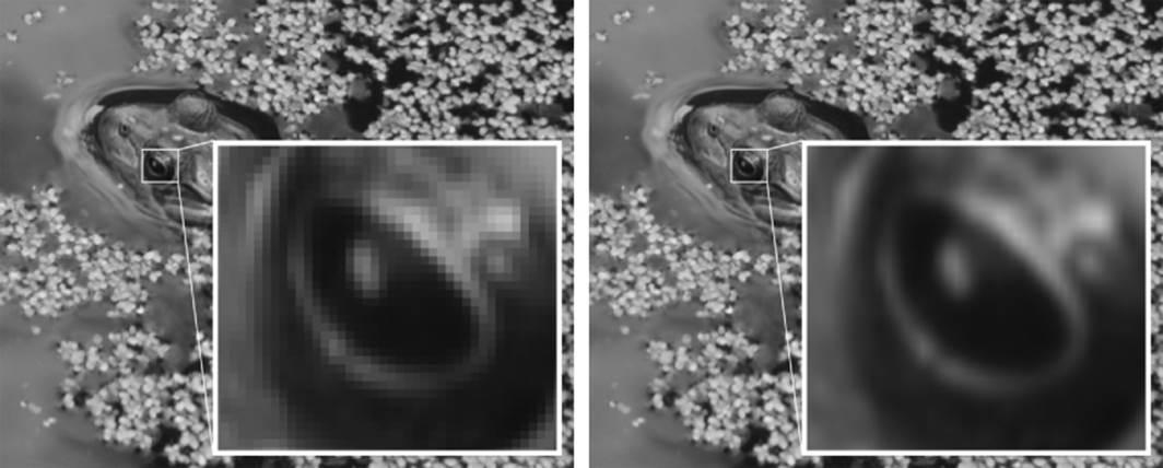
Figure 5.7: Texture filtering — nearest (left) and linear (right)
Linear filtering requires more work than nearest neighbor but often is worth the extra overhead. On today’s commodity hardware, the extra cost of linear filtering is usually zero. Linear filtering works by not taking the nearest texel to the texture coordinate, but by applying the weightedaverage of the texels surrounding the texture coordinate (a linear interpolation). For this interpolated fragment to match the texel color exactly, the texture coordinate needs to fall directly in the center of the texel. Linear filtering is characterized by “fuzzy” graphics when a texture is stretched. This fuzziness, however, often lends a more realistic and less artificial look than the jagged blocks of the nearest neighbor filtering mode. A contrasting example is shown on the right of Figure 5.7. You can set linear filtering simply enough by using the following lines:
glSamplerParameteri(sampler, GL_TEXTURE_MIN_FILTER, GL_LINEAR);
glSamplerParameteri(sampler, GL_TEXTURE_MAG_FILTER, GL_LINEAR);
Mipmaps
Mipmapping is a powerful texturing technique that can improve both the rendering performance and the visual quality of a scene. It does this by addressing two common problems with standard texture mapping. The first is an effect called scintillation (aliasing artifacts) that appears on the surface of objects rendered very small on-screen compared to the relative size of the texture applied. Scintillation can be seen as a sort of sparkling that occurs as the sampling area on a texture map moves disproportionately to its size on the screen. The negative effects of scintillation are most noticeable when the camera or the objects are in motion.
The second issue is more performance related but is due to the same scenario that leads to scintillation. That is, a large amount of texture memory is used to store the texture, but it is accessed very sparsely as adjacent fragments on the screen access texels that are disconnected in texture space. This causes texturing performance to suffer greatly as the size of the texture increases and the sparsity of access becomes greater.
The solution to both of these problems is to simply use a smaller texture map. However, this solution then creates a new problem: When near the same object, it must be rendered larger, and a small texture map will then be stretched to the point of creating a hopelessly blurry or blocky textured object. The solution to both of these issues is mipmapping. Mipmapping gets its name from the Latin phrase multum in parvo, which means “many things in a small place.” In essence, you load not only a single image into the texture object, but a whole series of images from largest to smallest into a single “mipmapped” texture. OpenGL then uses a new set of filter modes to choose the best-fitting texture or textures for the given geometry. At the cost of some extra memory (and possibly considerably more processing work), you can eliminate scintillation and the texture memory processing overhead for distant objects simultaneously, while maintaining higher resolution versions of the texture available when needed.
A mipmapped texture consists of a series of texture images, each one-half the size on each axis or one-fourth the total number of pixels of the previous image. This scenario is shown in Figure 5.8. Mipmap levels do not have to be square, but the halving of the dimensions continues until the last image is 1 × 1 texel. When one of the dimensions reaches 1, further divisions occur on the other dimension only. For 2D textures, using a square set of mipmaps requires about one-third more memory than not using mipmaps at all.
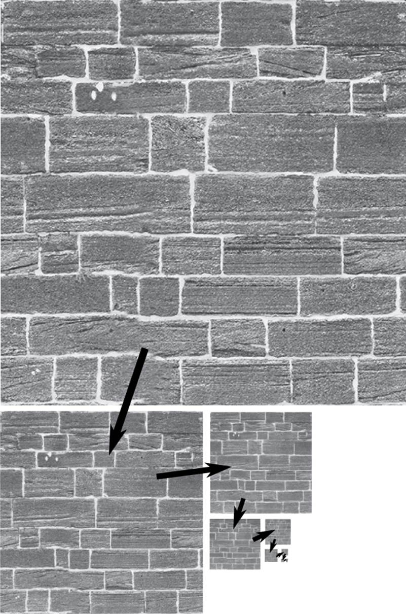
Figure 5.8: A series of mipmapped images
Mipmap levels are loaded with glTexSubImage2D() (for 2D textures). Now the level parameter comes into play because it specifies which mip level the image data is for. The first level is 0, then 1, 2, and so on. If mipmapping is not being used, you would usually use only level 0. When you allocate your texture with glTexStorage2D() (or the appropriate function for the type of texture you’re allocating), you can set the number of levels to include in the texture in the levels parameter. Then, you can use mipmapping with the levels present in the texture. You can further constrain the number of mipmap levels that will be used during rendering by setting the base and maximum levels to be used with the GL_TEXTURE_BASE_LEVEL and GL_TEXTURE_MAX_LEVEL texture parameters. For example, if you want to specify that only mip levels 0 through 4 should be accessed, you callglTexParameteri twice, as shown here:
glTexParameteri(GL_TEXTURE_2D, GL_TEXTURE_BASE_LEVEL, 0);
glTexParameteri(GL_TEXTURE_2D, GL_TEXTURE_MAX_LEVEL, 4);
Mipmap Filtering
Mipmapping adds a new twist to the two basic texture filtering modes GL_NEAREST and GL_LINEAR by giving four permutations for mipmapped filtering modes. They are listed in Table 5.7.
Table 5.7. Texture Filters, Including Mipmapped Filters
Just loading the mip levels with glTexStorage2D() does not by itself enable mipmapping. If the texture filter is set to GL_LINEAR or GL_NEAREST, only the base texture level is used, and any mip levels loaded are ignored. You must specify one of the mipmapped filters listed for the loaded mip levels to be used. The constants have the form GL_<FILTER>_MIPMAP_<SELECTOR>, where <FILTER> specifies the texture filter to be used on the mip level selected. The <SELECTOR> specifies how the mip level is selected; for example, NEAREST selects the nearest matching mip level. Using LINEAR for the selector creates a linear interpolation between the two nearest mip levels, which is again filtered by the chosen texture filter.
Which filter you select varies depending on the application and the performance requirements at hand. GL_NEAREST_MIPMAP_NEAREST, for example, gives very good performance and low aliasing (scintillation) artifacts, but nearest neighbor filtering is often not visually pleasing.GL_LINEAR_MIPMAP_NEAREST is often used to speed up games because a higher quality linear filter is used, but a fast selection (nearest) is made between the different-sized mip levels available. Note that you can only use the GL_<*>_MIPMAP_<*> filter modes for the GL_TEXTURE_MIN_FILTER setting — the GL_TEXTURE_MAG_FILTER setting must always be one of GL_NEAREST or GL_NEAREST.
Using nearest as the mipmap selector (as in both examples in the preceding paragraph), however, can also leave an undesirable visual artifact. For oblique views, you can often see the transition from one mip level to another across a surface. It can be seen as a distortion line or a sharp transition from one level of detail to another. The GL_LINEAR_MIPMAP_LINEAR and GL_NEAREST_MIPMAP_LINEAR filters perform an additional interpolation between mip levels to eliminate this transition zone, but at the extra cost of substantially more processing overhead. TheGL_LINEAR_MIPMAP_LINEAR filter is often referred to as trilinear mipmapping and, although there are more advanced techniques for image filtering, produces very good results.
Generating Mip Levels
As mentioned previously, mipmapping for 2D textures requires approximately one-third more texture memory than just loading the base texture image. It also requires that all the smaller versions of the base texture image be available for loading. Sometimes this can be inconvenient because the lower resolution images may not necessarily be available to either the programmer or the end user of your software. While having precomputed mip levels for your textures yields the very best results, it is convenient and somewhat common to have OpenGL generate the textures for you. You can generate all the mip levels for a texture once you loaded level zero with the function glGenerateMipmap():
void glGenerateMipmap(GLenum target);
The target parameter can be GL_TEXTURE_1D, GL_TEXTURE_2D, GL_TEXTURE_3D, GL_TEXTURE_CUBE_MAP, GL_TEXTURE_1D_ARRAY, or GL_TEXTURE_2D_ARRAY (more on these last three later). The quality of the filter used to create the smaller textures may vary widely from implementation to implementation. In addition, generating mipmaps on the fly may not be any faster than actually loading prebuilt mipmaps. This is something to think about in performance-critical applications. For the very best visual quality (as well as for consistency), you should load your own pregenerated mipmaps.
Mipmaps in Action
The example program tunnel shows off mipmapping as described in this chapter and demonstrates visually the different filtering and mipmap modes. This sample program loads three textures at startup and then switches between them to render a tunnel. The pre-filtered images that make up the textures are stored in the .KTX files containing the texture data. The tunnel has a brick wall pattern with different materials on the floor and ceiling. The output from tunnel is shown in Figure 5.9 with the texture minification mode set to GL_LINEAR_MIPMAP_LINEAR. As you can see, the texture becomes blurrier as you get further down the tunnel.
Figure 5.9: A tunnel rendered with three textures and mipmapping
Texture Wrap
Normally, you specify texture coordinates between 0.0 and 1.0 to map out the texels in a texture map. If texture coordinates fall outside this range, OpenGL handles them according to the current texture wrapping mode specified in the sampler object. You can set the wrap mode for each component of the texture coordinate individually by calling glSamplerParameteri() with GL_TEXTURE_WRAP_S, GL_TEXTURE_WRAP_T, or GL_TEXTURE_WRAP_R as the parameter name. The wrap mode can then be set to one of the following values: GL_REPEAT, GL_MIRRORED_REPEAT, GL_CLAMP_TO_EDGE, orGL_CLAMP_TO_BORDER. The value of GL_TEXTURE_WRAP_S affects 1D, 2D, and 3D textures; GL_TEXTURE_WRAP_T affects only 2D and 3D textures; and GL_TEXTURE_WRAP_R affects only 3D textures.
The GL_REPEAT wrap mode simply causes the texture to repeat in the direction in which the texture coordinate has exceeded 1.0. The texture repeats again for every integer texture coordinate. This mode is useful for applying a small tiled texture to large geometric surfaces. Well-done seamless textures can lend the appearance of a seemingly much larger texture, but at the cost of a much smaller texture image. The GL_MIRRORED_REPEAT mode is similar, but as each component of the texture passes 1.0, it starts moving back towards the origin of the texture until it reaches 2.0, at which point the pattern repeats. it is The other modes do not repeat, but are “clamped” — thus their name.
If the only implication of the wrap mode is whether the texture repeats, you would need only two wrap modes: repeat and clamp. However, the texture wrap mode also has a great deal of influence on how texture filtering is done at the edges of the texture maps. For GL_NEAREST filtering, there are no consequences to the wrap mode because the texture coordinates are always snapped to some particular texel within the texture map. However, the GL_LINEAR filter takes an average of the pixels surrounding the evaluated texture coordinate, and this creates a problem for texels that lie along the edges of the texture map. This problem is resolved quite neatly when the wrap mode is GL_REPEAT. The texel samples are simply taken from the next row or column, which in repeat mode wraps back around to the other side of the texture. This mode works perfectly for textures that wrap around an object and meet on the other side (such as spheres).
The clamped texture wrap mode offers a couple of options for the way texture edges are handled. For GL_CLAMP_TO_BORDER, the needed texels are taken from the texture border color (which can be set by passing GL_TEXTURE_BORDER_COLOR to glSamplerParameterfv()). The GL_CLAMP_TO_EDGEwrap mode forces texture coordinates out of range to be sampled along the last row or column of valid texels.
Figure 5.10 shows a simple example of the various texture wrapping modes. The same mode is used for both the S and T components of the texture coordinates. The four squares in the image have the same texture applied to them, but with different texture wrapping modes applied. The texture is a simple square with nine arrows pointing up and to the left, with a bright band around the top and right edges. For the top left square, the GL_CLAMP_TO_BORDER mode is used. The border color has been set to a dark color and it is clear that when OpenGL ran out of texture data, it used the dark color instead. However, in the bottom left square, the GL_CLAMP_TO_EDGE mode is used. In this case, the bright band is continued to the top and right of the texture data.
Figure 5.10: Example of texture coordinate wrapping modes
The bottom right square is drawn using the GL_REPEAT mode, which wraps the texture over and over. As you can see, there are several copies of our arrow texture, and all the arrows are pointing in the same direction. Compare this to the square on the top right of Figure 5.10. It is using theGL_MIRRORED_REPEAT mode and as you can see, the texture has been repeated across the square. However, the first copy of the image is the right way around, then the next copy is flipped, the next copy is the right way around again, and so on.
Array Textures
Previously we discussed the idea that multiple textures could be accessed at once via different texture units. This is extremely powerful and useful as your shader can gain access to several texture objects at the same time by declaring multiple sampler uniforms. We can actually take this a bit further by using a feature called array textures. With an array texture, you can load up several 1D, 2D, or cube map images into a single texture object. The concept of having more than one image in a single texture is not new. This happens with mipmapping, as each mip level is a distinctimage, and with cube mapping, where each face of the cube map has its own image and even its own set of mip levels. With texture arrays, however, you can have a whole array of texture images bound to a single texture object and then index through them in the shader, thus greatly increasing the amount of texture data available to your application at any one time.
Most texture types have an array equivalent. You can create 1D and 2D array textures, and even cube map array textures. However, you can’t create a 3D array texture as this is not supported by OpenGL. As with cube maps, array textures can have mip maps. Another interesting thing to note is that if you were to create an array of sampler uniforms in your shader, the value you use to index into that array must be uniform. However, with a texture array, each lookup into the texture map can come from a different element of the array. In part to distinguish between elements of an array of textures and a single element of an array texture, the elements are usually referred to as layers.
You may be wondering what the difference between a 2D array texture and a 3D texture is (or a 1D array texture and a 2D texture, for that matter). The biggest difference is probably that no filtering is applied between the layers of an array texture. Also, the maximum number of array texture layers supported by an implementation may be greater than the maximum 3D texture size, for example.
Loading a 2D Array Texture
To create a 2D array, simply create a new texture object bound to the GL_TEXTURE_2D_ARRAY target, allocate storage for it using glTexStorage3D(), and then load the images into it using one or more calls to glTexSubImage3D(). Notice the use of the 3D versions of the texture storage and data functions. These are required because the depth and z coordinates passed to them are interpreted as the array element, or layer. Simple code to load a 2D array texture is shown in Listing 5.40.
GLuint tex;
glGenTextures(1, &tex);
glBindTexture(GL_TEXTURE_2D_ARRAY, tex);
glTexStorage3D(GL_TEXTURE_2D_ARRAY,
8,
GL_RGBA8,
256,
256,
100);
for (int i = 0; i < 100; i++)
{
glTexSubImage3D(GL_TEXTURE_2D_ARRAY,
0,
0, 0,
i,
256, 256,
1,
GL_RGBA,
GL_UNSIGNED_BYTE,
image_data[i]);
}
Listing 5.40: Initializing an array texture
Conveniently, the .KTX file format supports array textures, and so the book’s loader code can load them directly from disk. Simply use sb6::ktx::file::load to load an array texture from a file.
To demonstrate texture arrays, we create a program that renders a large number of cartoon aliens raining on the screen. The sample uses an array texture where each slice of the texture holds one of 64 separate images of an alien. The array texture is packed into a single .KTX file calledalienarray.ktx, which we load into a single texture object. To render the alien rain, we draw hundreds of instances of a four-vertex triangle strip that makes a screen-aligned quad. Using the instance number as the index into the texture array gives each quad a different texture, even though they are all drawn with the same command. Additionally, we use a uniform buffer to store a per-instance orientation, x offset, and y offset, which are set up by the application.
In this case, our vertex shader uses no vertex attributes and is shown in its entirety in Listing 5.41.
#version 430 core
layout (location = 0) in int alien_index;
out VS_OUT
{
flat int alien;
vec2 tc;
} vs_out;
struct droplet_t
{
float x_offset;
float y_offset;
float orientation;
float unused;
};
layout (std140) uniform droplets
{
droplet_t droplet[256];
};
void main(void)
{
const vec2[4] position = vec2[4](vec2(-0.5, -0.5),
vec2( 0.5, -0.5),
vec2(-0.5, 0.5),
vec2( 0.5, 0.5));
vs_out.tc = position[gl_VertexID].xy + vec2(0.5);
float co = cos(droplet[alien_index].orientation);
float so = sin(droplet[alien_index].orientation);
mat2 rot = mat2(vec2(co, so),
vec2(-so, co));
vec2 pos = 0.25 * rot * position[gl_VertexID];
gl_Position = vec4(pos.x + droplet[alien_index].x_offset,
pos.y + droplet[alien_index].y_offset,
0.5, 1.0);
}
Listing 5.41: Vertex shader for the alien rain sample
In our vertex shader, the position of the vertex and its texture coordinate are taken from a hard-coded array. We calculate a per-instance rotation matrix, rot, allowing our aliens to spin. Along with the texture coordinate, vs_out.tc, we pass the value of gl_InstanceID (modulo 64) to the fragment shader via vs_out.alien. In the fragment shader, we simply use the incoming values to sample from the texture and write to our output. The fragment shader is shown in Listing 5.42.
#version 430 core
layout (location = 0) out vec4 color;
in VS_OUT
{
flat int alien;
vec2 tc;
} fs_in;
layout (binding = 0) uniform sampler2DArray tex_aliens;
void main(void)
{
color = texture(tex_aliens, vec3(fs_in.tc, float(fs_in.alien)));
}
Listing 5.42: Fragment shader for the alien rain sample
Accessing Texture Arrays
In the fragment shader (shown in Listing 5.42) we declare our sampler for the 2D array texture, sampler2DArray. To sample this texture we use the texture function as normal, but pass in a three-component texture coordinate. The first two components of this texture coordinate, the s and tcomponents, are used as typical two-dimensional texture coordinates. The third component, the p element, is actually an integer index into the texture array. Recall we set this in the vertex shader, and it is going to vary from 0 to 63, with a different value for each alien.
The complete rendering loop for the alien rain sample is shown in Listing 5.43.
void render(double currentTime)
{
static const GLfloat black[] = { 0.0f, 0.0f, 0.0f, 0.0f };
float t = (float)currentTime;
glViewport(0, 0, info.windowWidth, info.windowHeight);
glClearBufferfv(GL_COLOR, 0, black);
glUseProgram(render_prog);
glBindBufferBase(GL_UNIFORM_BUFFER, 0, rain_buffer);
vmath::vec4 * droplet =
(vmath::vec4 *)glMapBufferRange(
GL_UNIFORM_BUFFER,
0,
256 * sizeof(vmath::vec4),
GL_MAP_WRITE_BIT |
GL_MAP_INVALIDATE_BUFFER_BIT);
for (int i = 0; i < 256; i++)
{
droplet[i][0] = droplet_x_offset[i];
droplet[i][1] = 2.0f - fmodf((t + float(i)) *
droplet_fall_speed[i], 4.31f);
droplet[i][2] = t * droplet_rot_speed[i];
droplet[i][3] = 0.0f;
}
glUnmapBuffer(GL_UNIFORM_BUFFER);
int alien_index;
for (alien_index = 0; alien_index < 256; alien_index++)
{
glVertexAttribI1i(0, alien_index);
glDrawArrays(GL_TRIANGLE_STRIP, 0, 4);
}
}
Listing 5.43: Rendering loop for the alien rain sample
As you can see, there is only a simple loop around one drawing command in our rendering function. On each frame, we update the values of the data in the rain_buffer buffer object, which we use to store our per-droplet values. Then, we execute a loop of 256 calls to glDrawArrays(), which will draw 256 individual aliens. On each iteration of the loop, we update the alien_index input to the vertex shader. Note that we use the glVertexAttribI*() 1i variant of glVertexAttrib*() as we are using an integer input to our vertex shader. The final output of the alien rain sample program is shown in Figure 5.11.
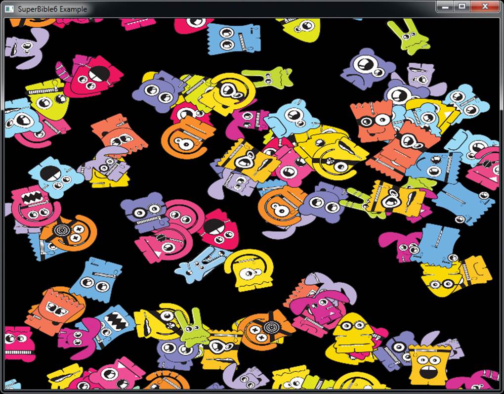
Figure 5.11: Output of the alien rain sample
Writing to Textures in Shaders
A texture object is a collection of images that, when the mipmap chain is included, support filtering, texture coordinate wrapping, and so on. Not only does OpenGL allow you to read from textures with all of those features, but it also allows you to read from and write to textures directly in your shaders. Just as you use a sampler variable in shaders to represent an entire texture and the associated sampler parameters (whether from a sampler object or from the texture object itself), you can use an image variable to represent a single image from a texture.
Image variables are declared just like sampler uniforms. There are several types of image variables that represent different data types and image dimensionalities. Table 5.8 shows the image types available to OpenGL.
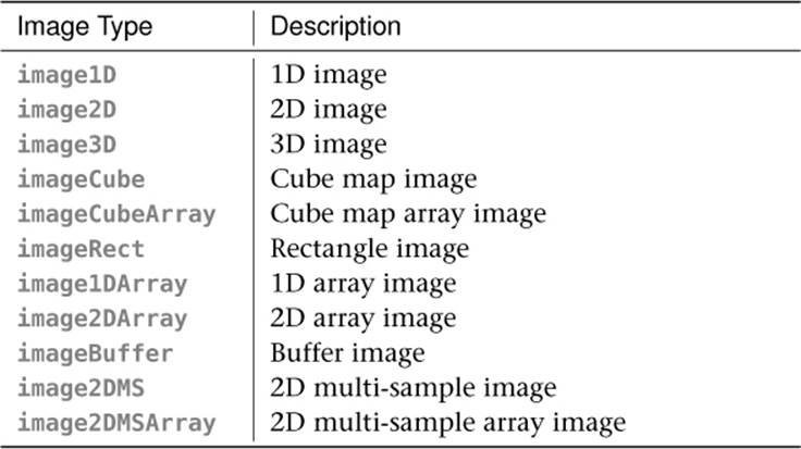
Table 5.8. Image Types
First, you need to declare an image variable as a uniform so that you can associate it with an image unit. Such a declaration generally looks like
uniform image2D my_image;
Once you have an image variable, you can read from it using the imageLoad function and write into it using the imageStore function. Both of these functions are overloaded, which means that there are multiple versions of each of them for various parameter types. The versions for the image2Dtype are
vec4 imageLoad(readonly image2D image, ivec2 P);
void imageStore(image2D image, ivec2 P, vec4 data);
The imageLoad() function will read the data from image at the coordinates specified in P and return it to your shader. Similarly, the imageStore() function will take the values you provide in data and store them into image at P. Notice that the type of P is an integer type (an integer vector for the case of 2D iamges). This is just like the texelFetch() function — no filtering is performed for loads and filtering really doesn’t make sense for stores. The dimension of P and the return type of the function depend on the type of the image parameter.
Just as with sampler types, image variables can represent floating-point data stored in images. However, it’s also possible to store signed and unsigned integer data in images, in which case the image type is prefixed with a i or u (as in iimage2D and uimage2D), respectively. When an integer image variable is used, the return type of the imageLoad function and the data type of the data parameter to imageStore change appropriately. For example, we have
ivec4 imageLoad(readonly iimage2D image, ivec2 P);
void imageStore(iimage2D image, ivec2 P, ivec4 data);
uvec4 imageLoad(readonly uimage2D image, ivec2 P);
void imageStore(uimage2D image, ivec2 P, uvec4 data);
To bind a texture for load and store operations, you need to bind it to an image unit using the glBindImageTexture() function, whose prototype is
void glBindImageTexture(GLuint unit,
GLuint texture,
GLint level,
GLboolean layered,
GLint layer,
GLenum access,
GLenum format);
The function looks like it has a lot of parameters, but they’re all fairly self-explanatory. First, the unit parameter is a zero-based index of the image unit5 to which you want to bind the image. Next, the texture parameter is the name of a texture object that you’ve created usingglGenTextures() and allocated storage for with glTexStorage2D() (or the appropriate function for the type of texture you’re using). level specifies which mipmap level you want to access in your shader, starting with zero for the base level and progressing to the number of mipmap levels in the image.
5. Note that there is no glActiveImageUnit function and there is no selector for image units. You can just bind an image to a unit directly.
The layered parameter should be set to GL_FALSE if you want to bind a single layer of an array texture as a regular 1D or 2D image, in which case the layer parameter specifies the index of that layer. Otherwise, layered should be set to GL_TRUE, and a whole level of an array texture will be bound to the image unit (with layer being ignored).
Finally, the access and format parameters describe how you will use the data in the image. access should be one of GL_READ_ONLY, GL_WRITE_ONLY, or GL_READ_WRITE to say that you plan to only read, only write, or to do both to the image, respectively. The format parameter specifies what format the data in the image should be interpreted as. There is a lot of flexibility here, with the only real requirement being that the image’s internal format (the one you specified in glTexStorage2D()) is in the same class as the one specified in the format parameter. Table 5.9 lists the acceptable image formats and their classes.
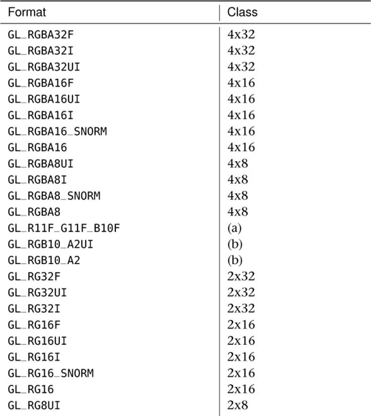
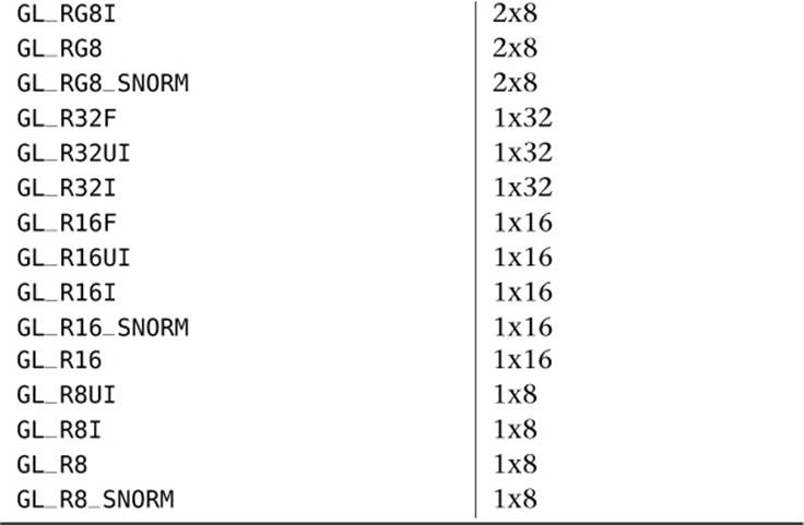
Table 5.9. Image Data Format Classes
Referring to Table 5.9, you can see that the GL_RGBA32F, GL_RGBA32I, and GL_RGBA32UI formats are in the same format class (4x32), which means that you can take a texture that has a GL_RGBA32F internal format and bind one of its levels to an image unit using the GL_RGBA32I or GL_RGBA32UI image formats. When you store into an image, the appropriate number of bits from your source data are chopped off and written to the image as is. However, if you want to read from an image, you must also supply a matching image format using a format layout qualifier in your shader code.
The GL_R11F_G11F_B10F format, which has the marker (a) for its format class, and GL_RGB10_A2UI and GL_RGB10_A2, which have the marker (b) for their format class, have their own special classes. GL_R11F_G11F_B10F is not compatible with anything else, and GL_RGB10_A2UI and GL_RGB10_A2 are only compatible with each other.
The appropriate format layout qualifiers for each of the various image formats are shown in Table 5.10.
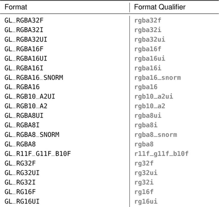
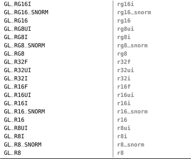
Table 5.10. Image Data Format Classes
Listing 5.44 shows an example fragment shader that copies data from one image to another using image loads and stores, logically inverting that data along the way.
#version 430 core
// Uniform image variables:
// Input image - note use of format qualifier because of loads
layout (binding = 0, rgba32ui) readonly uniform uimage2D image_in;
// Output image
layout (binding = 1) uniform writeonly uimage2D image_out;
void main(void)
{
// Use fragment coordinate as image coordinate
ivec2 P = ivec2(gl_FragCoord.xy);
// Read from input image
uvec4 data = imageLoad(image_in, P);
// Write inverted data to output image
imageStore(image_out, P, ~data);
}
Listing 5.44: Fragment shader performing image loads and stores
Obviously, the shader shown in Listing 5.44 is quite trivial. However, the power of image loads and stores is that you can include any number of them in a single shader and their coordinates can be anything. This means that a fragment shader is not limited to writing out to a fixed location in the framebuffer, but can write anywhere in an image, and write to multiple images by using multiple image uniforms. Furthermore, it allows any shader stage to write data into images, not just fragment shaders. Be aware, though that with this power comes a lot of responsibility. It’s perfectly easy for your shader to trash its own data — if multiple shader invocations write to the same location in an image, it’s not well defined what will happen unless you use atomics, which are described in the context of images in the next section.
Atomic Operations on Images
Just as with shader storage blocks described in the section “Atomic Memory Operations,” you can perform atomic operations on data stored in images. Again, an atomic operation is a sequence of a read, a modification, and a write that must be indivisible in order to achieve the desired result. Also, like atomic operations on members of a shader storage block, atomic operations on images are performed using a number of built-in functions in GLSL. These functions are listed in Table 5.11.
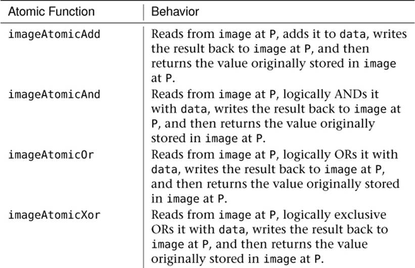
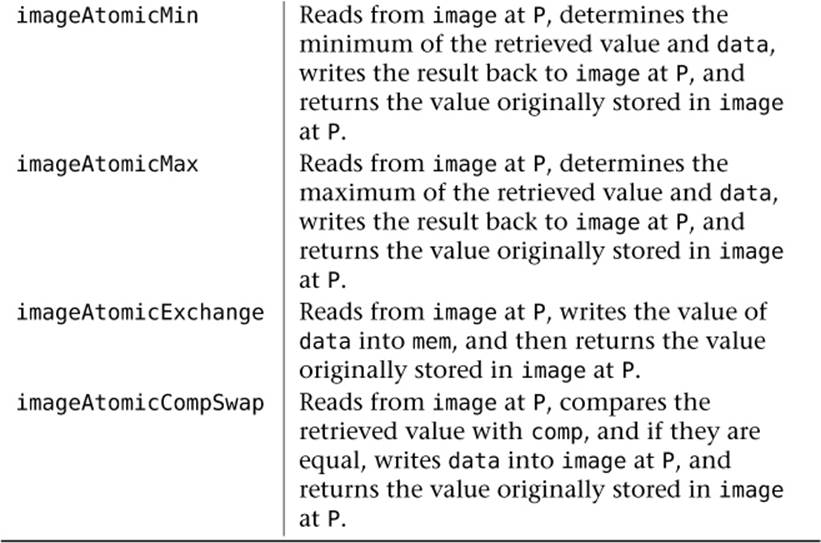
Table 5.11. Atomic Operations on Images
For all of the functions listed in Table 5.11 except for imageAtomicCompSwap, the parameters are an image variable, a coordinate, and a piece of data. The dimension of the coordinate depends on the type of image variable. 1D images use a single integer coordinate, 2D images and 1D array images take a 2D integer vector (i.e., ivec2), and 3D images and 2D array images take a 3D integer vector (i.e., ivec3).
For example, we have
uint imageAtomicAdd(uimage1D image, int P, uint data);
uint imageAtomicAdd(uimage2D image, ivec2 P, uint data);
uint imageAtomicAdd(uimage3D image, ivec3 P, uint data);
and so on. The imageAtomicCompSwap is unique in that it takes an additional parameter, comp, which it compares with the existing content in memory. If the value of comp is equal to the value already in memory, then it is replaced with the value of data. The prototypes of imageAtomicCompSwapinclude
uint imageAtomicCompSwap(uimage1D image, int P, uint comp, uint data);
uint imageAtomicCompSwap(uimage2D image, ivec2 P, uint comp, uint data);
uint imageAtomicCompSwap(uimage3D image, ivec3 P, uint comp, uint data);
All of the atomic functions return the data that was originally in memory before the operation was performed. This is useful if you wish to append data to a list, for example. To do this, you would simply determine how many items you want to append to the list, call imageAtomicAdd with the number of elements and then start writing your new data into memory at the location that it returns. Note that while you can’t add an arbitrary number to an atomic counter (and the number of atomic counters supported in a single shader is usually not great), you can do similar things with shader storage buffers.
The memory you write to could be a shader storage buffer or another image variable. If the image containing the “filled count” variables is pre-initialized to zero, then the first shader invocation to attempt to append to the list will receive zero and write there, the next invocation will receive whatever the first added, the next will receive whatever the third added, and so on.
Another application for atomics is constructing data structures such as linked lists in memory. To build a linked list from a shader, you need three pieces of storage — the first is somewhere to store the list items, the second is somewhere to store the item count, and the third is the “head pointer,” which is the index of the last item on in the list. Again, you can use a shader storage buffer to store items for the linked list, an atomic counter to store the current item count, and an image to store the head pointer for the list(s). To append an item to the list, you would follow three steps:
1. Increment the atomic counter, and retrieve its previous value, which is returned by atomicCounterIncrement.
2. Use imageAtomicExchange to exchange the updated counter value with the current head pointer.
3. Store your data into your data store. The structure for each element includes a next index, which you fill with the previous value of the head pointer retrieved in step 2.
If the “head pointer” image is a 2D image the size of the framebuffer, then you can use this method to create a per-pixel list of fragments. You can later walk this list and perform whatever operations you like. The shader shown in Listing 5.45 demonstrates how to append fragments to a linked list stored in a shader storage buffer using a 2D image to store the head pointers and an atomic counter to keep the fill count.
#version 430 core
// Atomic counter for filled size
layout (binding = 0, offset = 0) uniform atomic_uint fill_counter;
// 2D image to store head pointers
layout (binding = 0) uniform uimage2D head_pointer;
// Shader storage buffer containing appended fragments
struct list_item
{
vec4 color;
float depth;
int facing;
uint next;
};
layout (binding = 0, std430) buffer list_item_block
{
list_item item[];
};
// Input from vertex shader
in VS_OUT
{
vec4 in;
} fs_in;
void main(void)
{
ivec2 P = ivec2(gl_FragCoord.xy);
uint index = atomicCounterIncrement(fill_counter);
uint old_head = imageAtomicExchange(head_pointer, P, index);
item[index].color = fs_in.color;
item[index].depth = gl_FragCoord.z;
item[index].facing = gl_FrontFacing ? 1 : 0;
item[index].next = old_head;
}
Listing 5.45: Filling a linked list in a fragment shader
You might notice the use of the gl_FrontFacing built-in variable. This is a Boolean input to the fragment shader whose value is generated by the back-face culling stage that is described in “Primitive Assembly, Clipping, and Rasterization” back in Chapter 3, “Following the Pipeline.” Even if back-face culling is disabled, this variable will still contain true if the polygon is considered front facing and false otherwise.
Before executing this shader, the head pointer image is cleared to a known value that can’t possibly be the index of an item in the list (such as the maximum value of an unsigned integer), and the atomic counter is reset to zero. The first item appended will be item zero, that value will be written to the head pointer, and its next index will contain the reset value of the head pointer image. The next value appended to the list will be at index 1, which is written to the head pointer, the old value of which (0) is written to the next index, and so on. The result is that the head pointer image contains the index of the last item appended to the list, and each item contains the index of the previous one appended. Eventually, the next index of an item will be the value originally used to clear the head image, which indicates that the end of the list.
To traverse the list, we load the index of the first item in it from the head pointer image and read it from the shader storage buffer. For each item, we simply follow the next index until we reach the end of the list, or until the maximum number of fragments have been traversed (which protects us from accidentally running off the end of the list). The shader shown in Listing 5.46 shows an example of this. The shader walks the linked list, keeping a running total of the depth of the fragments stored for each pixel. The depth value of front-facing primitives is added to the running total, and the depth value of back-facing primitives is subtracted from the total. The result is the total filled depth of the interior of convex objects, which can be used to render volumes and other filled spaces.
#version 430 core
// 2D image to store head pointers
layout (binding = 0, r32ui) coherent uniform uimage2D head_pointer;
// Shader storage buffer containing appended fragments
struct list_item
{
vec4 color;
float depth;
int facing;
uint next;
};
layout (binding = 0, std430) buffer list_item_block
{
list_item item[];
};
layout (location = 0) out vec4 color;
const uint max_fragments = 10;
void main(void)
{
uint frag_count = 0;
float depth_accum = 0.0;
ivec2 P = ivec2(gl_FragCoord.xy);
uint index = imageLoad(head_pointer, P).x;
while (index != 0xFFFFFFFF && frag_count < max_fragments)
{
list_item this_item = item[index];
if (this_item.facing != 0)
{
depth_accum -= this_item.depth;
}
else
{
depth_accum += this_item.depth;
}
index = this_item.next;
frag_count++;
}
depth_accum *= 3000.0;
color = vec4(depth_accum, depth_accum, depth_accum, 1.0);
}
Listing 5.46: Traversing a linked list in a fragment shader
The result of rendering with the shaders of Listings 5.45 and 5.46 is shown in Figure 5.12.
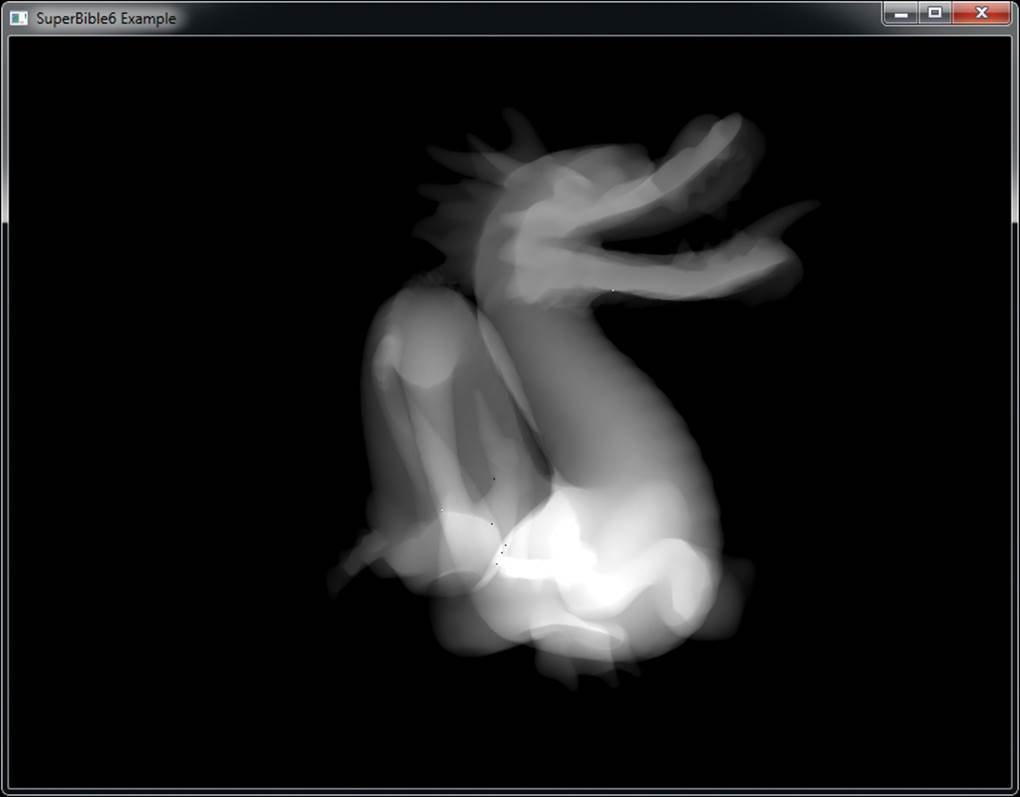
Figure 5.12: Resolved per-fragment linked lists
Synchronizing Access to Images
As images represent large regions of memory and we have just explained how to write directly into images from your shaders, you may have guessed that we’ll now explain the memory barrier types that you can use to synchronize access to that memory. Just as with buffers and atomic counters, you can call
glMemoryBarrier(GL_SHADER_IMAGE_ACCESS_BIT);
You should call glMemoryBarrier() with the GL_SHADER_IMAGE_ACCESS_BIT set when something has written to an image that you want read from images later — including other shaders.
Similarly, there is a version of the GLSL memoryBarrier() function, memoryBarrierImage(), that ensures that operations on images from inside your shader are completed before it returns.
Texture Compression
Textures can take up an incredible amount of space! Some modern games can easily use 1GB of texture data in a given level. That’s a lot of data! Where do you put it all? Textures are an important part to making rich, realistic, and impressive scenes, but if you can’t load all of the data onto the GPU, your rendering will be slow if not impossible. One way to deal with storing and using a large amount of texture data is to compress the data. Compressed textures have two major benefits. First, they reduce the amount of storage space required for image data. Although the texture formats supported by OpenGL are not generally not compressed as aggressively as in formats such as JPEG, they do provide substantial space benefits. The second (and possibly more important) benefit is that because the graphics processor needs to read less data when fetching from a compressed texture, less memory bandwidth is required when compressed textures are used.
There are a number of compressed texture formats supported by OpenGL. All OpenGL implementations support at least the compression schemes listed in Table 5.12.
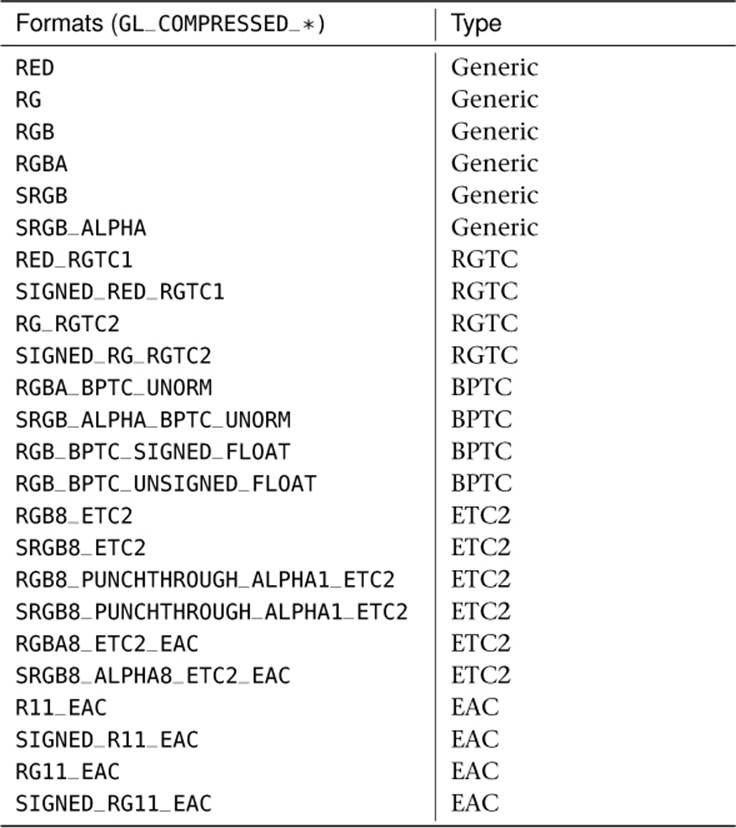
Table 5.12. Native OpenGL Texture Compression Formats
The first six formats listed in Table 5.12 are generic and allow the OpenGL driver to decide what compression mechanism to use. This means your driver can use the format that best meets current conditions. The catch is that it is implementation specific, and although your code will work on many platforms, the result of rendering with them might not be the same.
The RGTC (Red-Green Texture Compression) format breaks a texture image into 4 × 4 texel blocks, compressing the individual channels within that block using a series of codes. This compression mode works only for one- and two-channel signed and unsigned textures, and only for certain texel formats. You don’t need to worry about the exact compression scheme unless you are planning on writing a compressor. Just note that space savings from using RGTC is 50%.
The BPTC (Block Partitioned Texture Compression) format also breaks textures up into blocks of 4 × 4 texels, each represented as 128 bits (16 bytes) of data in memory. The blocks are encoded using a rather complex scheme that essentially comprises a pair of endpoints and a representation of the position on a line between those two endpoints. It allows the endpoints to be manipulated to generate a variety of values as output for each texel. The BPTC formats are capable of compressing 8-bit per-channel normalized data and 32-bit per-channel floating-point data. The compression ratio for BPTC formats ranges from 25% for RGBA floating-point data to 33% for RGB 8-bit data.
The other formats listed, Ericsson Texture Compression (ETC2) and Ericsson Alpha6 Compression (EAC) are low-bandwidth formats that are also7 available in OpenGL ES 3.0. They are designed for extremely low bit-per-pixel applications such as those found in mobile devices that have substantially less memory bandwidth than the high-performance GPUs found in desktop and workstation computers.
6. Although this is the official acronym, it’s a bit of a misnomer as EAC can be used for more than just alpha.
7. The EAC and ETC2 formats were added to OpenGL 4.3 in an effort to drive convergence between desktop and mobile versions of the API, and at time of writing, few if any desktop GPUs actually support them natively, with most OpenGL implementations decompressing the data you give them. Use them with caution.
Your implementation may also support other compressed formats such as S3TC8 and ETC1. You should check for the availability of formats not required by OpenGL before attempting to use them. The best way to do this is to check for support of the related extension. For example, if your implementation of OpenGL supports the S3TC, it will advertise the GL_EXT_texture_compression_s3tc extension string.
8. S3TC is also known as the earlier versions of the DXT format.
Using Compression
You can ask OpenGL to compress a texture in some formats when you load it, although it’s strongly recommended to compress textures yourself and store the compressed texture in a file. If OpenGL does support compression for your selected format, all you have to do is request that the internal format be one of the compressed formats and OpenGL will take your uncompressed data and compress it as the texture image is loaded. There is no real difference in how you use compressed textures and uncompressed textures. The GPU handles the conversion when it samples from the texture. Many imaging tools used for creating textures and other images allow you to save your data directly in a compressed format.
The .KTX file format allows compressed data to be stored in it, and the book’s texture loader will load compressed images transparently to your application. You can check whether a texture is compressed by calling glGetTexLevelParameteriv() with one of two parameters. As one option, you can check the GL_TEXTURE_INTERNAL_FORMAT parameter of the texture and explicitly test whether it’s one of the compressed formats. To do this, either keep a lookup table of recognized formats in your application or call glGetInternalFormativ() with the parameter GL_TEXTURE_COMPRESSED. Alternatively, simply pass the GL_TEXTURE_COMPRESSED parameter directly to glGetTexLevelParameteriv(), which will return GL_TRUE if the texture has compressed data in it and GL_FALSE otherwise.
Once you have loaded a texture using a non-generic compressed internal format, you can get the compressed image back by calling glGetCompressedTexImage(). Just pick the texture target and mipmap level you are interested in. Because you may not know how the image is compressed or what format is used, you should check the image size to make sure you have enough room for the whole surface. You can do this by calling glGetTexParameteriv() and passing the GL_TEXTURE_COMPRESSED_IMAGE_SIZE token.
Glint imageSize = 0;
glGetTexParameteriv(GL_TEXTURE_2D,
GL_TEXTURE_COMPRESSED_IMAGE_SIZE,
&imageSize);
void *data = malloc(imageSize);
glGetCompressedTexImage(GL_TEXTURE_2D, 0, data);
If you wish to load compressed texture images yourself rather than using the book’s .KTX loader, you can call glTexStorage2D() or glTexStorage3D() with the desired compressed internal format to allocate storage for the texture, and then call glCompressedTexSubImage2D() orglCompressedTexSubImage3D() to upload data into it. When you do this, you need to ensure that the xoffset, yoffset, and other parameters obey texture format specific rules. In particular, most texture compression formats compress blocks of texels. These blocks are usually sizes such as 4× 4 texels. The regions that you update with glCompressedTexSubImage2D() need to line up on block boundaries for these formats to work.
Shared Exponents
Although shared exponent textures are not technically a compressed format in the truest sense, they do allow you to use floating-point texture data while saving storage space. Instead of storing an exponent for each of the R, G, and B values, shared exponent formats use the same exponent value for the whole texel. The fractional and exponential parts of each value are stored as integers and then assembled when the texture is sampled. For the format GL_RGB9_E5, 9 bits are used to store each color and 5 bits are the common exponent for all channels. This format packs three floating-point values into 32 bits; that’s a savings of 67%! To make use of shared exponents, you can get the texture data directly in this format from a content creation tool or write a converter that compresses your float RGB values into a shared exponent format.
Texture Views
Usually, when you’re using textures, you’ll know ahead of time what format your textures are, what you’re going to use them for and your shaders will match the data they’re fetching. For instance, a shader that’s expecting to read from a 2D array texture might declare a sampler uniform as asampler2DArray. Likewise, a shader that’s expecting to read from an integer format texture might declare a corresponding sampler as isampler2D. However, there may be times when the textures you create and load might not match what your shaders expect. In this case, you can use texture views to re-use the texture data in one texture object with another. This has two main use cases (although there are certainly many more):
• A texture view can be used to “pretend” that a texture of one type is actually a texture of a different type. For example, you can take a 2D texture and create a view of it that treats it as a 2D array texture with only one layer.
• A texture view can be used to pretend that the data in the texture object is actually a different format than what is really stored in memory. For example, you might take a texture with an internal format of GL_RGBA32F (i.e., four 32-bit floating-point components per texel) and create a view of it that sees them as GL_RGBA32UI (four 32-bit unsigned integers per texel) so that you can get at the individual bits of the texels.
Of course, you can do both of these things at the same time — that is, take a texture and create a view of it with both a different format and different type.
Creating Texture Views
To create a view of a texture, we use the glTextureView() function, whose prototype is
void glTextureView(GLuint texture,
GLenum target,
GLuint origtexture,
GLenum internalformat,
GLuint minlevel,
GLuint numlevels,
GLuint minlayer,
GLuint numlayers);
The first parameter, texture, is the name of the texture object you’d like to make into a view. You should get this name from a call to glGenTextures(). Next, target specifies what type of texture you’d like to create. This can be pretty much any of the texture targets (GL_TEXTURE_1D,GL_TEXTURE_CUBE_MAP, or GL_TEXTURE_2D_ARRAY, for example), but it must be compatible with the type of the original texture, whose name is given in origtexture. The compatibility between various targets is given in Table 5.13.
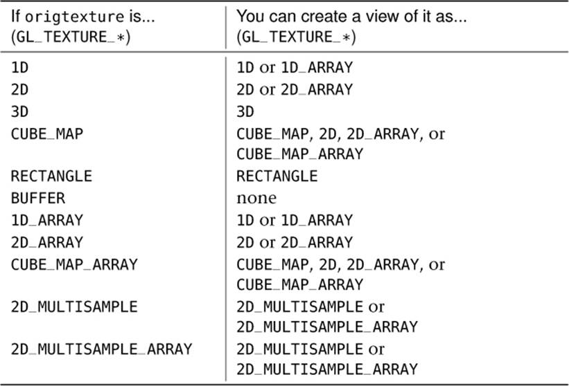
Table 5.13. Texture View Target Compatibility
As you can see, for most texture targets you can at least create a view of the texture with the same target. The exception is buffer textures as these are essentially already views of a buffer object — you can simply attach the same buffer object to another buffer texture to get another view of its data.
The internalformat parameter specifies the internal format for the new texture view. This must be compatible with the internal format of the original texture. This can be tricky to understand, so we’ll explain it in a moment.
The last four parameters allow you to make a view of a subset of the original texture’s data. The minlevel and numlevels parameter specify the first mipmap level and number of mipmap levels to include in the view. This allows you to create a texture view that represents part of an entire mipmap pyramid of another texture. For example, to create a texture that represented just the base level (level 0) of another texture, you can set minlevel to 0 and numlevels to 1. To create a view that represented the 4 lowest resolution mipmaps of a 10-level texture, you would set minlevel to 6 and numlevels to 4.
Similarly, minlayer and numlayers are used to create a view of a subset of the layers of an array texture. For instance, if you want to create an array texture view that represents the middle 4 layers of a 20-layer array texture, you can set minlayer to 8 and numlayers to 4. Whatever you choose for the minlevel, numlevels, minlayer, and numlayers parameters, they must be consistent with the source and destination textures. For example, if you want to create a non-array texture view representing a single layer of an array texture, you must set minlayer to a layer that actually exists in the source texture and numlayers to 1 because the destination doesn’t have any layers (rather, it effectively has 1 layer).
We mentioned that the internal format of the source texture and the new texture view (specified in the internalformat parameter) must be compatible with one another. To be compatible, two formats must be in the same class. There are several format classes, and they are listed, along with the internal formats that are members of that class, in Table 5.14.
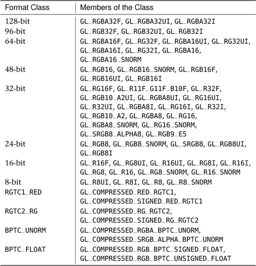
Table 5.14. Texture View Format Compatibility
In addition to formats that match each other’s classes, you can always create a view of a texture with the same format as the original — even for formats that are not listed in Table 5.14.
Once you have created a view of a texture, you can use it like any other texture of the new type. For instance, if you have a 2D array texture, and you create a 2D non-array texture view of one of its layers, you can call glTexSubImage2D() to put data into the view, and the same data will end up in the corresponding layer of the array texture. As another example, you can create a 2D non-array texture view of a single layer of a 2D array texture and access it from a sampler2D uniform in a shader. Likewise, you could create a single-layer 2D array texture view of a 2D non-array texture and access that from a sampler2DArray uniform in a shader.
Summary
In this chapter, you have learned about how OpenGL deals with the vast amounts of data required for graphics rendering. At the start of the pipeline, you saw how to automatically feed your vertex shaders with data using buffer objects. We also discussed methods of getting constant values, known as uniforms, into your shaders — first using buffers and then using the default uniform block. This block is where the uniforms that represent textures, images, and storage buffers live too, and we used them to show you how to directly read and write images to and from textures and buffers using your shader code. You saw how to take a texture and pretend that part of it’s actually a different type of texture, possibly with a different data format. You also learned about atomic operations, which touched on the massively parallel nature of modern graphics processors.