OpenGL SuperBible: Comprehensive Tutorial and Reference, Sixth Edition (2013)
Part II: In Depth
Chapter 7. Vertex Processing and Drawing Commands
What You’ll Learn in This Chapter
• How to get data from your application into the front of the graphics pipeline
• What the various OpenGL drawing commands are and what their parameters do
• How your transformed geometry gets into your application’s window
In Chapter 3, we followed the OpenGL pipeline from start to finish, producing a simple application that exercised every shader stage with a minimal example that was just enough to make it do something. We even showed you a simple compute shader that did nothing at all! However, the result of all this was a single tessellated triangle broken into points. Since then, you have learned some of the math involved in 3D computer graphics, have seen how to set up the pipeline to do more than draw a single triangle, and have a deeper introduction to GLSL, the OpenGL Shading Language. In this chapter, we dig deeper into the first couple of stages of the OpenGL pipeline — that is, vertex assembly and vertex shading. We’ll see how drawing commands are structured and how they can be used to send work into the OpenGL pipeline, and how that ends up in primitives being produced ready for rasterization.
Vertex Processing
The first programmable stage in the OpenGL pipeline (i.e., one that you can write a shader for) is the vertex shader. Before the shader runs, OpenGL will fetch the inputs to the vertex shader in the vertex fetch stage, which we will describe first. Your vertex shader’s responsibility is to set the position1 of the vertex that will be fed to the next stage in the pipeline. It can also set a number of other user-defined and built-in outputs that further describe the vertex to OpenGL.
1. Under certain circumstances, you may even omit this.
Vertex Shader Inputs
The first step in any OpenGL graphics pipeline is the the vertex fetch stage, unless the configuration does not require any vertex attributes, as was the case in some of our earliest examples. This stage runs before your vertex shader and is responsible for forming its inputs. You have been introduced to the glVertexAttribPointer() function, and we have explained how it hooks data in buffers up to vertex shader inputs. Now, we’ll take a closer look at vertex attributes.
In the example programs presented thus far, we’ve only used a single vertex attribute and have filled it with four-component floating-point data, which matches the data types we have used for our uniforms, uniform blocks, and hard-coded constants. However, OpenGL supports a large number of vertex attributes, and each can have its own format, data type, number of components, and so on. Also, OpenGL can read the data for each attribute from a different buffer object. glVertexAttribPointer() is a handy way to set up virtually everything about a vertex attribute. However, it can actually be considered more of a helper function that sits on top of a few lower level functions: glVertexAttribFormat(), glVertexAttribBinding(), and glBindVertexBuffer(). Their prototypes are
void glVertexAttribFormat(GLuint attribindex, GLint size,
GLenum type, GLboolean normalized,
GLuint relativeoffset);
void glVertexAttribBinding(GLuint attribindex,
GLuint bindingindex);
void glBindVertexBuffer(GLuint bindingindex,
GLuint buffer,
GLintptr offset,
GLintptr stride);
In order to understand how these functions work, first, let’s consider a simple vertex shader fragment that declares a number of inputs. In Listing 7.1, notice the use of the location layout qualifier to set the locations of the inputs explicitly in the shader code.
#version 430 core
// Declare a number of vertex attributes
layout (location = 0) in vec4 position;
layout (location = 1) in vec3 normal;
layout (location = 2) in vec2 tex_coord;
// Note that we intentionally skip location 3 here
layout (location = 4) in vec4 color;
layout (location = 5) in int material_id;
Listing 7.1: Declaration of a Multiple Vertex Attributes
The shader fragment in Listing 7.1 declares five inputs, position, normal, tex_coord, color, and material_id. Now, consider that we are using a data structure to represent our vertices that is defined in C as
typedef struct VERTEX_t
{
vmath::vec4 position;
vmath::vec3 normal;
vmath::vec2 tex_coord;
GLubyte color[3];
int material_id;
} VERTEX;
Notice that our vertex structure in C mixes use of vmath types and plain old data (for color).
The first attribute is pretty standard and should be familiar to you — it’s the position of the vertex, specified as a four-component floating-point vector. To describe this input using the glVertexAttribFormat() function, we would set size to 4 and type to GL_FLOAT. The second, the normal of the geometry at the vertex, is in normal and would be passed to glVertexAttribFormat() with size set to 3 and, again, type set to GL_FLOAT. Likewise, tex_coord can be used as a two-dimensional texture coordinate and might be specified by setting size to 2 and type to GL_FLOAT.
Now, the color input to the vertex shader is declared as a vec4, but the color member of our VERTEX structure is actually an array of 3 bytes. Both the size (number of elements) and the data type are different. OpenGL can convert the data for you as it reads it into the vertex shader. To hook our 3-byte color member up to our four-component vertex shader input, we call glVertexAttribFormat() with size set to 3 and type set to GL_UNSIGNED_BYTE. This is where the normalized parameter comes in. As you probably know, the range of values representable by an unsigned byte is 0 to 255. However, that’s not what we want in our vertex shader. There, we want to represent colors as values between 0.0 and 1.0. If you set normalized to GL_TRUE, then OpenGL will automatically divide through each component of the input by the maximum possible representable positive value,normalizing it.
Because two’s-complement numbers are able to represent a greater magnitude negative number than a positive number, this can place one value below the -1.0 (-128 for GLbyte, -32,768 for GLshort, and -2,147,483,648 for GLint). Those most negative numbers are treated specially and are clamped to the floating-point value -1.0 during normalization. If normalized is GL_FALSE, then the value will be converted directly to floating point and presented to the vertex shader. In the case of unsigned byte data (like color), this means that the values will be between 0.0 and 255.0.
Table 7.1 shows the tokens that can be used for the type parameter, their corresponding OpenGL type, and the range of values that they can represent.
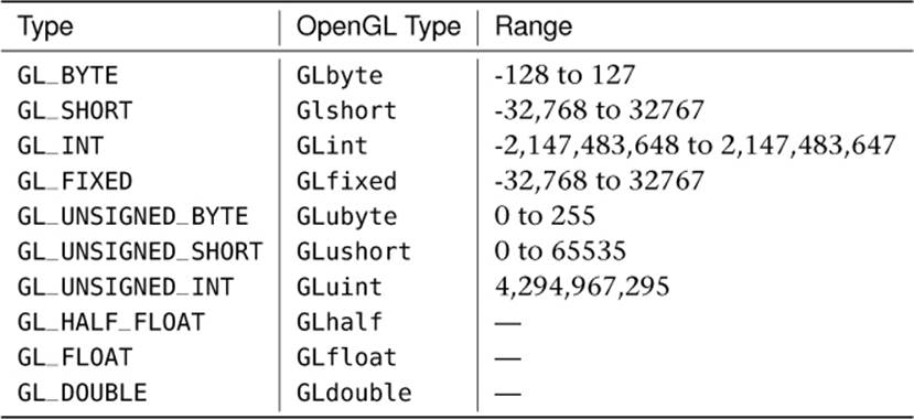
Table 7.1. Vertex Attribute Types
In Table 7.1, the floating-point types (GLhalf, GLfloat, and GLdouble) don’t have ranges because they can’t be normalized. The GLfixed type is a special case. It represents fixed-point data that is made up of 32 bits with the binary point at position 16 (halfway through the number), and as such, it is treated as one of the floating-point types and cannot be normalized.
In addition to the scalar types shown in Table 7.1, glVertexAttribFormat() also supports several packed data formats that use a single integer to store multiple components. The two packed data formats supported by OpenGL are GL_UNSIGNED_INT_2_10_10_10_REV and GL_INT_2_10_10_10_REV, which both represent four components packed into a single 32-bit word.
The GL_UNSIGNED_INT_2_10_10_10_REV format provides 10 bits for each of the x, y, and z components of the vector and only 2 bits for the w component, which are all treated as unsigned quantities. This gives a range of 0 to 1023 for each of x, y, and z and 0 to 3 for w. Likewise, theGL_INT_2_10_10_10_REV format provides 10 bits for x, y, and z and 2 bits for w, but in this case, each component is treated as a signed quantity. That means that while x, y, and z have a range of -512 to 511, w may range from -2 to 1. While this may not seem terribly useful, there are a number of use cases for three-component vectors with more than 8 bits of precision (24 bits in total), but that do not require 16 bits of precision (48 bits in total), and even though those last two bits might be wasted, 10 bits of precision per component provides what is needed.
When one of the packed data types (GL_UNSIGNED_INT_2_10_10_10_REV or GL_INT_2_10_10_10_REV) is specified, then size must be set either to 4 or to the special value GL_BGRA. This applies an automatic swizzle to the incoming data to reverse the order of the r, g, and b (which are equivalent to the x, y, and z) components of the incoming vectors. This provides compatibility with data stored in that order2 without needing to modify your shaders.
2. The BGRA ordering is quite common in some image formats and is the default ordering used by some graphics APIs.
Finally, returning to our example vertex declaration, we have the material_id field, which is an integer. In this case, because we want to pass an integer value as is to the vertex shader, we’ll use a variation on the glVertexAttribFormat(), glVertexAttribIFormat(), whose prototype is
void glVertexAttribIFormat(GLuint attribindex,
GLint size,
GLenum type,
GLuint relativeoffset);
Again, the attribindex, size, type, and relativeoffset parameters specify the attribute index, number of components, type of those components, and the offset from the start of the vertex of the attribute that’s being set up. However, you’ll notice that the normalized parameter is missing. That’s because this version of glVertexAttribFormat() is only for integer types — type must be one of the integer types (GL_BYTE, GL_SHORT, GL_INT, one of their unsigned counterparts, or one of the packed data formats), and integer inputs to a vertex shader are never normalized. Thus, the complete code to describe our vertex format is
// position
glVertexAttribFormat(0, 4, GL_FLOAT, GL_FALSE, offsetof(VERTEX, position));
// normal
glVertexAttribFormat(1, 3, GL_FLOAT, GL_FALSE, offsetof(VERTEX, normal));
// tex_coord
glVertexAttribFormat(2, 2, GL_FLOAT, GL_FALSE, offsetof(VERTEX, texcoord));
// color[3]
glVertexAttribFormat(4, 3, GL_UNSIGNED_BYTE, GL_TRUE, offsetof(VERTEX, color));
// material_id
glVertexAttribIFormat(5, 1, GL_INT, offsetof(VERTEX, material_id));
Now that you’ve set up the vertex attribute format, you need to tell OpenGL which buffers to read the data from. If you recall our discussion of uniform blocks and how they map to buffers, you can apply similar logic to vertex attributes. Each vertex shader can have any number of input attributes (up to an implementation-defined limit), and OpenGL can provide data for them by reading from any number of buffers (again, up to a limit). Some vertex attributes can share space in a buffer; others may reside in different buffer objects. Rather than individually specifying which buffer objects are used for each vertex shader input, we can instead group inputs together and associate groups of them with a set of buffer binding points. Then, when you change the buffer bound to one of these binding points, it will change the buffer used to supply data for all of the attributes that are mapped to that binding point.
To establish the mapping between vertex shader inputs and buffer binding points, you can call glVertexAttribBinding(). The first parameter to glVertexAttribBinding(), attribindex, is the index of the vertex attribute, and the second parameter, bindingindex, is the buffer binding point index. In our example, we’re going to store all of the vertex attributes in a single buffer. To set this up, we’d simply call glVertexAttribBinding() once for each attribute and specify zero for the bindingindex parameter each time:
void glVertexAttribBinding(0, 0); // position
void glVertexAttribBinding(1, 0); // normal
void glVertexAttribBinding(2, 0); // tex_coord
void glVertexAttribBinding(4, 0); // color
void glVertexAttribBinding(5, 0); // material_id
However, we could establish a more complex binding scheme. Let’s say, for example, that we wanted to store position, normal, and tex_coord in one buffer, color in a second, and material_id in a third. We could set this up as follows:
void glVertexAttribBinding(0, 0); // position
void glVertexAttribBinding(1, 0); // normal
void glVertexAttribBinding(2, 0); // tex_coord
void glVertexAttribBinding(4, 1); // color
void glVertexAttribBinding(5, 2); // material_id
Finally, we need to bind a buffer object to each of the binding points that is used by our mapping. To do this, we call glBindVertexBuffer(). This function takes four parameters, bindingindex, buffer, offset, and stride. The first is the index of the buffer binding point that you want to bind the buffer, and the second is the name of the buffer object that you’re going to bind. offset is an offset into the buffer object where the vertex data starts, and stride is the distance, in bytes, between the start of each vertex’s data in the buffer. If your data is tightly packed (i.e., there are no gaps between the vertices), you can just set this to the total size of your vertex data (which would be sizeof(VERTEX) in our example); otherwise, you’ll need to add the size of the gaps to the size of the vertex data.
Vertex Shader Outputs
After your vertex shader has decided what to do with the vertex data, it must send it to its outputs. We have already discussed the gl_Position built-in output variable, and have shown you how you can create your own outputs from shaders that can be used to pass data into the following stages. Along with gl_Position, OpenGL also defines a couple more output variables, gl_PointSize and gl_ClipDistance[], and wraps them up into an interface block called gl_PerVertex. Its declaration is
out gl_PerVertex
{
vec4 gl_Position;
float gl_PointSize;
float gl_ClipDistance[];
};
Again, you should be familiar with gl_Position. gl_ClipDistance[] is used for clipping, which will be described in some detail later in this chapter. The other output, gl_PointSize, is used for controlling the size of points that might be rendered.
Variable Point Sizes
By default, OpenGL will draw points with a size of a single fragment. However, as you saw way back in Chapter 2, you can change the size of points that OpenGL draws by calling glPointSize(). The maximum size that OpenGL will draw your points is implementation defined, but it will be least 64 pixels. You find out what the actual upper limit is by calling glGetIntegerv() to find the value of GL_POINT_SIZE_RANGE. This will actually write two integers to the output variable, so make sure you point it at an array of two integers. The first element of the array will be filled with the minimum point size (which will be at most 1), and the second element will be filled with the maximum point size.
Now, setting all of your points to be big blobs isn’t going to produce particularly appealing images. You can actually set the point size programmatically in the vertex shader (or whatever stage is last in the front end). To do this, write the desired value of the point diameter to the built-in variable gl_PointSize. Once you have a shader that does this, you need to tell OpenGL that you wish to use the size written to the point size variable. To do this, call
glEnable(GL_PROGRAM_POINT_SIZE);
A common use for this is to determine the size of a point based on its distance from the viewer. When you use the glPointSize() function to set the size of points, every point will have the same size no matter what their position is. By choosing a value for gl_PointSize, you can implement any function you wish, and each point produced by a single draw command can have a different size. This includes points generated in the geometry shader or by the tessellation engine when the tessellation evaluation shader specifies point_mode.
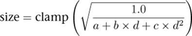
The following formula is often used to implement distance-based point size attenuation, where d is the distance of the point from the eye and a, b, and c are configurable parameters of a quadratic equation. You can store those in uniforms and update them with your application, or if you have a particular set of parameters in mind, you might want to make them constants in your vertex shader. For example, if you want a constant size, set a to a non-zero value and b and c to zero. If a and c are zero and b is non-zero, then point size will fall off linearly with distance. Likewise, if aand b are zero but c is non-zero, then point size will fall off quadratically with distance.
Drawing Commands
Until now, we have written every example using only a single drawing command — glDrawArrays(). OpenGL includes many drawing commands, however, and while some could be considered supersets of others, they can be generally categorized as either indexed or non-indexed and direct or indirect. Each of these will be covered in the next few sections.
Indexed Drawing Commands
The glDrawArrays() command is a non-indexed drawing command. That is, the vertices are issued in order, and any vertex data stored in buffers and associated with vertex attributes is simply fed to the vertex shader in the order that it appears in the buffer. An indexed draw, on the other hand, includes an indirection step that treats the data in each of those buffers as an array, and rather than index into that array sequentially, it reads from another array of indices, and after having read the index, OpenGL uses that to index into the array. To make an indexed drawing command work, you need to bind a buffer to the GL_ELEMENT_ARRAY_BUFFER target. This buffer will contain the indices of the vertices that you want to draw. Next, you call one of the indexed drawing commands, which all have the word Elements in their names. For example, glDrawElements() is the simplest of these functions and its prototype is
void glDrawElements(GLenum mode,
GLsizei count,
GLenum type,
const GLvoid * indices);
When you call glDrawElements(), mode and type have the same meaning as they do for glDrawArrays(). type specifies the type of data used to store each index and may be one of GL_UNSIGNED_BYTE to indicate one byte per index, GL_UNSIGNED_SHORT to indicate 16 bits per index, andGL_UNSIGNED_INT to indicate 32 bits per index. Although indices is defined as a pointer, it is actually interpreted as the offset into the buffer currently bound to the GL_ELEMENT_ARRAY_BUFFER binding where the first index is stored. Figure 7.1 shows how the indices specified by a call toglDrawElements() are used by OpenGL.
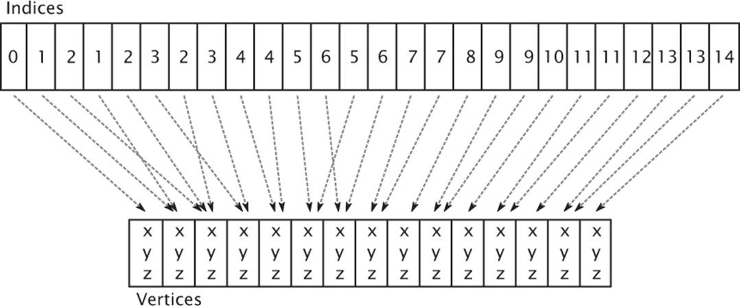
Figure 7.1: Indices used in an indexed draw
The glDrawArrays() and glDrawElements() commands are actually subsets of the complete functionality supported by the direct drawing commands of OpenGL. The set of the most generalized OpenGL drawing commands is given in Table 7.2 — all other OpenGL drawing commands can be expressed in terms of these functions.
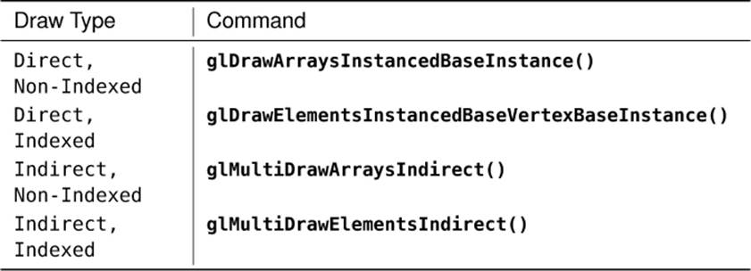
Table 7.2. Draw Type Matrix
Remember back to the spinning cube example in Chapter 5 and in particular to the geometry setup performed in Listing 5.20. To draw a cube, we drew 12 triangles (two for each face of the cube), and each one consumed 36 vertices. However, a cube really only has 8 corners, and so should only need 8 vertices of information, right? Well, we can use an indexed draw to greatly cut down the amount of vertex data, especially for geometry that has a lot of vertices. We can re-write the setup code of Listing 5.20 to only define the 8 corners of the cube, but to also define a set of 36 indices that tell OpenGL which corner to use for each vertex of each triangle. The new setup code looks like this:
static const GLfloat vertex_positions[] =
{
-0.25f, -0.25f, -0.25f,
-0.25f, 0.25f, -0.25f,
0.25f, -0.25f, -0.25f,
0.25f, 0.25f, -0.25f,
0.25f, -0.25f, 0.25f,
0.25f, 0.25f, 0.25f,
-0.25f, -0.25f, 0.25f,
-0.25f, 0.25f, 0.25f,
};
static const GLushort vertex_indices[] =
{
0, 1, 2,
2, 1, 3,
2, 3, 4,
4, 3, 5,
4, 5, 6,
6, 5, 7,
6, 7, 0,
0, 7, 1,
6, 0, 2,
2, 4, 6,
7, 5, 3,
7, 3, 1
};
glGenBuffers(1, &position_buffer);
glBindBuffer(GL_ARRAY_BUFFER, position_buffer);
glBufferData(GL_ARRAY_BUFFER,
sizeof(vertex_positions),
vertex_positions,
GL_STATIC_DRAW);
glVertexAttribPointer(0, 3, GL_FLOAT, GL_FALSE, 0, NULL);
glEnableVertexAttribArray(0);
glGenBuffers(1, &index_buffer);
glBindBuffer(GL_ELEMENT_ARRAY_BUFFER, index_buffer);
glBufferData(GL_ELEMENT_ARRAY_BUFFER,
sizeof(vertex_indices),
vertex_indices,
GL_STATIC_DRAW);
Listing 7.2: Setting up indexed cube geometry
As you can see from Listing 7.2, the total amount of data required to represent our cube is greatly reduced — it went from 108 floating-point values (36 triangles times 3 components each, which is 432 bytes) down to 24 floating-point values (just the 8 corners at 3 components each, which is 72 bytes) and 36 16-bit integers (another 72 bytes), for a total of 144 bytes, representing a reduction of two-thirds. To use the index data in vertex_indices, we need to bind a buffer to the GL_ELEMENT_ARRAY_BUFFER and put the indices in it just as we did with the vertex data. In Listing 7.2, we do that right after we set up the buffer containing vertex positions.
Once you have a set of vertices and their indices in memory, you’ll need to change your rendering code to use glDrawElements() (or one of the more advanced versions of it) instead of glDrawArrays(). Our new rendering loop for the spinning cube example is shown in Listing 7.3.
// Clear the framebuffer with dark green
static const GLfloat green[] = { 0.0f, 0.25f, 0.0f, 1.0f };
glClearBufferfv(GL_COLOR, 0, green);
// Activate our program
glUseProgram(program);
// Set the model-view and projection matrices
glUniformMatrix4fv(mv_location, 1, GL_FALSE, mv_matrix);
glUniformMatrix4fv(proj_location, 1, GL_FALSE, proj_matrix);
// Draw 6 faces of 2 triangles of 3 vertices each = 36 vertices
glDrawElements(GL_TRIANGLES, 36, GL_UNSIGNED_SHORT, 0);
Listing 7.3: Drawing indexed cube geometry
Notice that we’re still drawing 36 vertices, but now 36 indices will be used to index into an array of only 8 unique vertices. The result of rendering with the vertex index and position data in our two buffers and a call to glDrawElements() is identical to that shown in Figure 5.2.
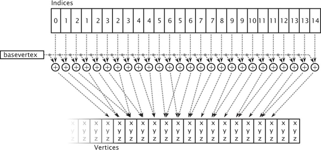
Figure 7.2: Base vertex used in an indexed draw
The Base Vertex
The first advanced version of glDrawElements() that takes an extra parameter is glDrawElementsBaseVertex(), whose prototype is
void glDrawElementsBaseVertex(GLenum mode,
GLsizei count,
GLenum type,
GLvoid * indices,
GLint basevertex);
When you call glDrawElementsBaseVertex(), OpenGL will fetch the vertex index from the buffer bound to the GL_ELEMENT_ARRAY_BUFFER and then add basevertex to it before it is used to index into the array of vertices. This allows you to store a number of different pieces of geometry in the same buffer and then offset into it using basevertex. Figure 7.2 shows how basevertex is added to vertices in an indexed drawing command.
As you can see from Figure 7.2, vertex indices are essentially fed into an addition operation, which adds the base vertex to it before OpenGL uses it to fetch the underlying vertex data. Clearly, if basevertex is zero, then glDrawElementsBaseVertex() is equivalent to glDrawElements(). In fact, we consider calling glDrawElements() as equivalent to calling glDrawElementsBaseVertex() with basevertex set to zero.
Combining Geometry using Primitive Restart
There are many tools out there that “stripify” geometry. The idea of these tools is that by taking “triangle soup,” which means a large collection of unconnected triangles, and attempting to merge it into a set of triangle strips, performance can be improved. This works because individual triangles are each represented by three vertices, but a triangle strip reduces this to a single vertex per triangle (not counting the first triangle in the strip). By converting the geometry from triangle soup to triangle strips, there is less geometry data to process, and the system should run faster. If the tool does a good job and produces a small number of long strips containing many triangles each, this generally works well. There has been a lot of research into this type of algorithm, and a new method’s success is measured by passing some well-known models through the new “stripifier” and comparing the number and average length of the strips generated by the new tool to those produced by current state-of-the-art stripifiers.
Despite all of this research, the reality is that a soup can be rendered with a single call to glDrawArrays() or glDrawElements(), but unless the functionality that is about to be introduced is used, a set of strips needs to be rendered with separate calls to OpenGL. This means that there is likely to be a lot more function calls in a program that uses stripified geometry, and if the stripping application hasn’t done a decent job or if the model just doesn’t lend well to stripification, this can eat any performance gains seen by using strips in the first place.
A feature that can help here is primitive restart. Primitive restart applies to the GL_TRIANGLE_STRIP, GL_TRIANGLE_FAN, GL_LINE_STRIP, and GL_LINE_LOOP geometry types. It is a method of informing OpenGL when one strip (or fan or loop) has ended and that another should be started. To indicate the position in the geometry where one strip ends and the next starts, a special marker is placed as a reserved value in the element array. As OpenGL fetches vertex indices from the element array, it checks for this special index value, and whenever it comes across it, it ends the current strip and starts a new one with the next vertex. This mode is disabled by default but can be enabled by calling
glEnable(GL_PRIMITIVE_RESTART);
and disabled again by calling
glDisable(GL_PRIMITIVE_RESTART);
When primitive restart mode is enabled, OpenGL watches for the special index value as it fetches them from the element array buffer and when it comes across it, stops the current strip and starts a new one. To set the index that OpenGL should watch for, call
glPrimitiveRestartIndex(index);
OpenGL watches for the value specified by index and uses that as the primitive restart marker. Because the marker is a vertex index, primitive restart is best used with indexed drawing functions such as glDrawElements(). If you draw with a non-indexed drawing command such asglDrawArrays(), the primitive restart index is simply ignored.
The default value of the primitive restart index is zero. Because that’s almost certainly the index of a real vertex that will be contained in the model, it’s a good idea to set the restart index to a new value whenever you’re using primitive restart mode. A good value to use is the maximum value representable by the index type you’re using (0xFFFFFFFF for GL_UNSIGNED_INT, 0xFFFF for GL_UNSIGNED_SHORT, and 0xFF for GL_UNSIGNED_BYTE) because you can be almost certain that it will not be used as a valid index of a vertex. Many stripping tools have an option to either create separate strips or to create a single strip with the restart index in it. The stripping tool may use a predefined index or output the index it used when creating the stripped version of the model (for example, one greater than the number of vertices in the model). You need to know this and set it using theglPrimitiveRestartIndex() function to use the output of the tool in your application. The primitive restart feature is illustrated in Figure 7.3.
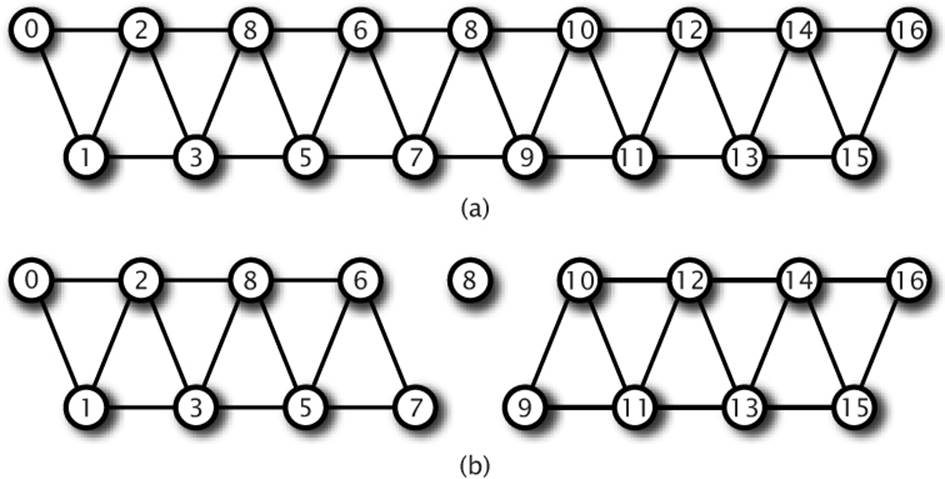
Figure 7.3: Triangle strips with and without primitive restart
In Figure 7.3, a triangle strip is pictured with the vertices marked with their indices. In (a), the strip is made up of 17 vertices, which produces a total of 15 triangles in a single, connected strip. By enabling primitive restart mode and setting the primitive restart index to 8, the 8th index (whose value is also 8) is recognized by OpenGL as the special restart marker, and the triangle strip is terminated at vertex 7. This is shown in (b). The actual position of vertex 8 is ignored because this is not seen by OpenGL as the index of a real vertex. The next vertex processed (vertex 9) becomes the start of a new triangle strip. So while 17 vertices are still sent to OpenGL, the result is that two separate triangle strips of 8 vertices and 6 triangles each are drawn.
Instancing
There will probably be times when you want to draw the same object many times. Imagine a fleet of starships, or a field of grass. There could be thousands of copies of what are essentially identical sets of geometry, modified only slightly from instance to instance. A simple application might just loop over all of the individual blades of grass in a field and render them separately, calling glDrawArrays() once for each blade and perhaps updating a set of shader uniforms on each iteration. Supposing each blade of grass were made up of a strip of four triangles, the code might look something like Listing 7.4.
glBindVertexArray(grass_vao);
for (int n = 0; n < number_of_blades_of_grass; n++)
{
SetupGrassBladeParameters();
glDrawArrays(GL_TRIANGLE_STRIP, 0, 6);
}
Listing 7.4: Drawing the same geometry many times
How many blades of grass are there in a field? What is the value of number_of_blades_of_grass? It could be thousands, maybe millions. Each blade of grass is likely to take up a very small area on the screen, and the number of vertices representing the blade is also very small. Your graphics card doesn’t really have a lot of work to do to render a single blade of grass, and the system is likely to spend most of its time sending commands to OpenGL rather than actually drawing anything. OpenGL addresses this through instanced rendering, which is a way to ask it to draw many copies of the same geometry.
Instanced rendering is a method provided by OpenGL to specify that you want to draw many copies of the same geometry with a single function call. This functionality is accessed through instanced rendering functions, such as
void glDrawArraysInstanced(GLenum mode,
GLint first,
GLsizei count,
GLsizei instancecount);
and
void glDrawElementsInstanced(GLenum mode,
GLsizei count,
GLenum type,
const void * indices,
GLsizei instancecount);
These two functions behave much like glDrawArrays() and glDrawElements(), except that they tell OpenGL to render instancecount copies of the geometry. The first parameters of each (mode, first, and count for glDrawArraysInstanced(), and mode, count, type, and indices forglDrawElementsInstanced()) take the same meaning as in the regular, non-instanced versions of the functions. When you call one of these functions, OpenGL makes any preparations it needs to draw your geometry (such as copying vertex data to the graphics card’s memory, for example) only once and then renders the same vertices many times.
If you set instancecount to one, then glDrawArraysInstanced() and glDrawElementsInstanced() will draw a single instance of your geometry. Obviously, this is equivalent to calling glDrawArrays() or glDrawElements(), but we normally state this equivalency the other way around — that is, we say that calling glDrawArrays() is equivalent to calling glDrawArraysInstanced() with instancecount set to one, and that, likewise, calling glDrawElements() is equivalent to calling glDrawElementsInstanced() with instancecount set to one. As we discussed earlier, though, calling glDrawElements() is also equivalent to calling glDrawElementsBaseVertex() with basevertex set to zero. In fact, there is another drawing command that combines both basevertex and instancecount together. This is glDrawElementsInstancedBaseVertex(), whose prototype is
void glDrawElementsInstancedBaseVertex(GLenum mode,
GLsizei count,
GLenum type,
GLvoid * indices,
GLsizei instancecount,
GLint basevertex);
So, in fact, calling glDrawElements() is equivalent to calling glDrawElementsInstancedBaseVertex() with instancecount set to one and basevertex set to zero, and likewise, calling glDrawElementsInstanced() is equivalent to calling glDrawElementsInstancedBaseVertex() withbasevertex set to zero.
Finally, just as we can pass basevertex to glDrawElementsBaseVertex() and glDrawElementsInstancedBaseVertex(), we can pass a baseinstance parameter to versions of the instanced drawing commands. These functions are glDrawArraysInstancedBaseInstance(),glDrawElementsInstancedBaseInstance(), and the exceedingly long glDrawElementsInstancedBaseVertexBaseInstance(), which takes both a basevertex and baseinstance parameter. Now we have introduced all of the direct drawing commands, it should be clear that they are all subsets of glDrawArraysInstancedBaseInstance() and glDrawElementsInstancedBaseVertexBaseInstance(), and that where they are missing, basevertex and baseinstance are assumed to be zero, and instancecount is assumed to be one.
If all that these functions did were send many copies of the same vertices to OpenGL as if glDrawArrays() or glDrawElements() had been called in a tight loop, they wouldn’t be very useful. One of the things that makes instanced rendering usable and very powerful is a special, built-in variable in GLSL named gl_InstanceID. The gl_InstanceID variable appears in the vertex as if it were a static integer vertex attribute. When the first copy of the vertices is sent to OpenGL, gl_InstanceID will be zero. It will then be incremented once for each copy of the geometry and will eventually reach instancecount - 1.
The glDrawArraysInstanced() function essentially operates as if the code in Listing 7.5 were executed.
// Loop over all of the instances (i.e., instancecount)
for (int n = 0; n < instancecount; n++)
{
// Set the gl_InstanceID attribute - here gl_InstanceID is a C variable
// holding the location of the "virtual" gl_InstanceID input.
glVertexAttrib1i(gl_InstanceID, n);
// Now, when we call glDrawArrays, the gl_InstanceID variable in the
// shader will contain the index of the instance that's being rendered.
glDrawArrays(mode, first, count);
}
Listing 7.5: Pseudo-code for glDrawArraysInstanced()
Likewise, the glDrawElementsInstanced() function operates similarly to the code in Listing 7.6.
for (int n = 0; n < instancecount; n++)
{
// Set the value of gl_InstanceID
glVertexAttrib1i(gl_InstanceID, n);
// Make a normal call to glDrawElements
glDrawElements(mode, count, type, indices);
}
Listing 7.6: Pseudo-code for glDrawElementsInstanced()
Of course, gl_InstanceID is not a real vertex attribute, and you can’t get a location for it by calling glGetAttribLocation(). The value of gl_InstanceID is managed by OpenGL and is very likely generated in hardware, meaning that it’s essentially free to use in terms of performance. The power of instanced rendering comes from imaginative use of this variable, along with instanced arrays, which are explained in a moment.
The value of gl_InstanceID can be used directly as a parameter to a shader function or to index into data such as textures or uniform arrays. To return to our example of the field of grass, let’s figure out what we’re going to do with gl_InstanceID to make our field not just be thousands of identical blades of grass growing out of a single point. Each of our grass blades is made out of a little triangle strip with four triangles in it, a total of just six vertices. It could be tricky to get them to all look different. However, with some shader magic, we can make each blade of grass look sufficiently different so as to produce an interesting output. We won’t go over the shader code here, but we will walk through a few ideas of how you can use gl_InstanceID to add variation to your scenes.
First, we need each blade of grass to have a different position; otherwise, they’ll all be drawn on top of each other. Let’s arrange the blades of grass more or less evenly. If the number of blades of grass we’re going to render is a power of 2, we can use half of the bits of gl_InstanceID to represent the x coordinate of the blade, and the other half to represent the z coordinate (our ground lies in the xz plane, with y being altitude). For this example, we render 220, or a little over a million, blades of grass (actually 1,048,576 blades, but who’s counting?). By using the ten least significant bits (bits 9 through 0) as the x coordinate and the ten most significant bits (19 through 10) as the z coordinate, we have a uniform grid of grass blades. Let’s take a look at Figure 7.4 to see what we have so far.
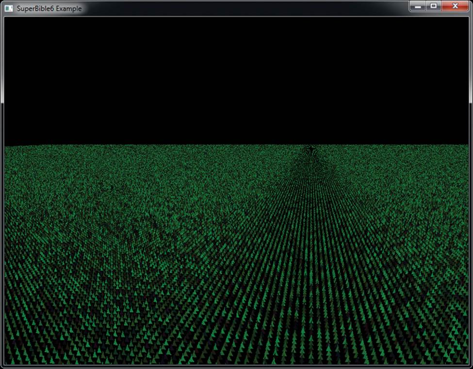
Figure 7.4: First attempt at an instanced field of grass
Our uniform grid of grass probably looks a little plain, as if a particularly attentive groundskeeper hand-planted each blade. What we really need to do is displace each blade of grass by some random amount within its grid square. That’ll make the field look a little less uniform. A simple way of generating random numbers is to multiply a seed value by a large number and take a subset of the bits of the resulting product and use it as the input to a function. We’re not aiming for a perfect distribution here, so this simple generator should do. Usually, with this type of algorithm, you’d reuse the seed value as input to the next iteration of the random number generator. In this case, though, we can just use gl_InstanceID directly as we’re really generating the next few numbers after gl_InstanceID in a pseudo-random sequence. By iterating over our pseudo-random function only a couple of times, we can get a reasonably random distribution. Because we need to displace in both x and z, we generate two successive random numbers from gl_InstanceID and use them to displace the blade of grass within the plane. Look at Figure 7.5 to see what we get now.
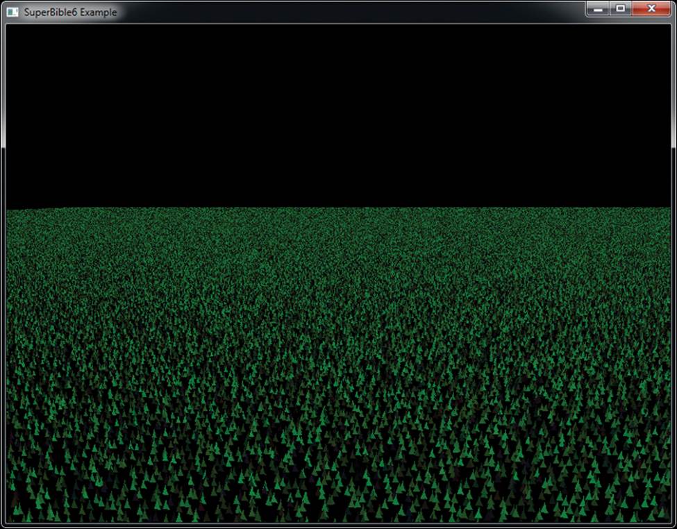
Figure 7.5: Slightly perturbed blades of grass
At this point, our field of grass is distributed evenly with random perturbations in position for each blade of grass. All the grass blades look the same, though. (Actually, we used the same random number generator to assign a slightly different color to each blade of grass just so that they’d show up in the figures.) We can apply some variation over the field to make each blade look slightly different. This is something that we’d probably want to have control over, so we use a texture to hold information about blades of grass.
You have an x and a z coordinate for each blade of grass that was calculated by generating a grid coordinate directly from gl_InstanceID and then generating a random number and displacing the blade within the xz plane. That coordinate pair can be used as a coordinate to look up a texel within a 2D texture, and you can put whatever you want in it. Let’s control the length of the grass using the texture. We can put a length parameter in the texture (let’s use the red channel) and multiply the y coordinate of each vertex of the grass geometry by that to make longer or shorter grass. A value of zero in the texture would produce very short (or nonexistent) grass, and a value of one would produce grass of some maximum length. Now you can design a texture where each texel represents the length of the grass in a region of your field. Why not draw a few crop circles?
Now, the grass is evenly distributed over the field, and you have control of the length of the grass in different areas. However, the grass blades are still just scaled copies of each other. Perhaps we can introduce some more variation. Next, we rotate each blade of grass around its axis according to another parameter from the texture. We use the green channel of the texture to store the angle through which the grass blade should be rotated around the y axis, with zero representing no rotation and one representing a full 360 degrees. We’ve still only done one texture fetch in our vertex shader, and still the only input to the shader is gl_InstanceID. Things are starting to come together. Take a look at Figure 7.6.
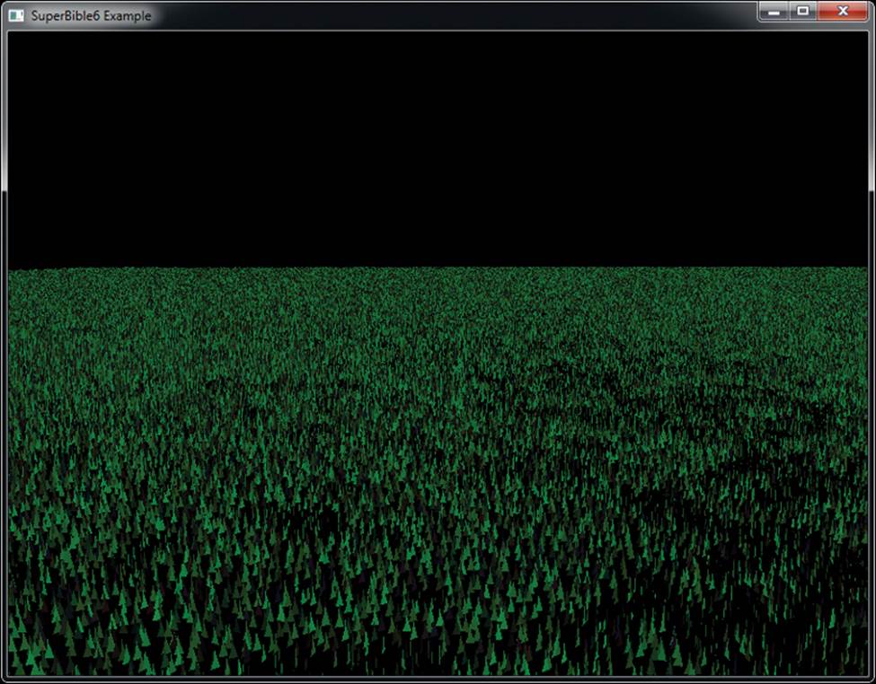
Figure 7.6: Control over the length and orientation of our grass
Our field is still looking a little bland. The grass just sticks straight up and doesn’t move. Real grass sways in the wind and gets flattened when things roll over it. We need the grass to bend, and we’d like to have control over that. Why not use another channel from the parameter texture (the blue channel) to control a bend factor? We can use that as another angle and rotate the grass around the x axis before we apply the rotation in the green channel. This allows us to make the grass bend over based on the parameter in the texture. Use zero to represent no bending (the grass stands straight up) and one to represent fully flattened grass. Normally, the grass will sway gently, and so the parameter will have a low value. When the grass gets flattened, the value can be much higher.
Finally, we can control the color of the grass. It seems logical to just store the color of the grass in a large texture. This might be a good idea if you want to draw a sports field with lines, markings, or advertising on it for example, but it’s fairly wasteful if the grass is all varying shades of green. Instead, let’s make a palette for our grass in a 1D texture and use the final channel within our parameter texture (the alpha channel) to store the index into that palette. The palette can start with an anemic looking dead-grass yellow at one end and a lush, deep green at the other end. Now we read the alpha channel from the parameter texture along with all the other parameters and use it to index into the 1D texture—a dependent texture fetch. Our final field is shown in Figure 7.7.
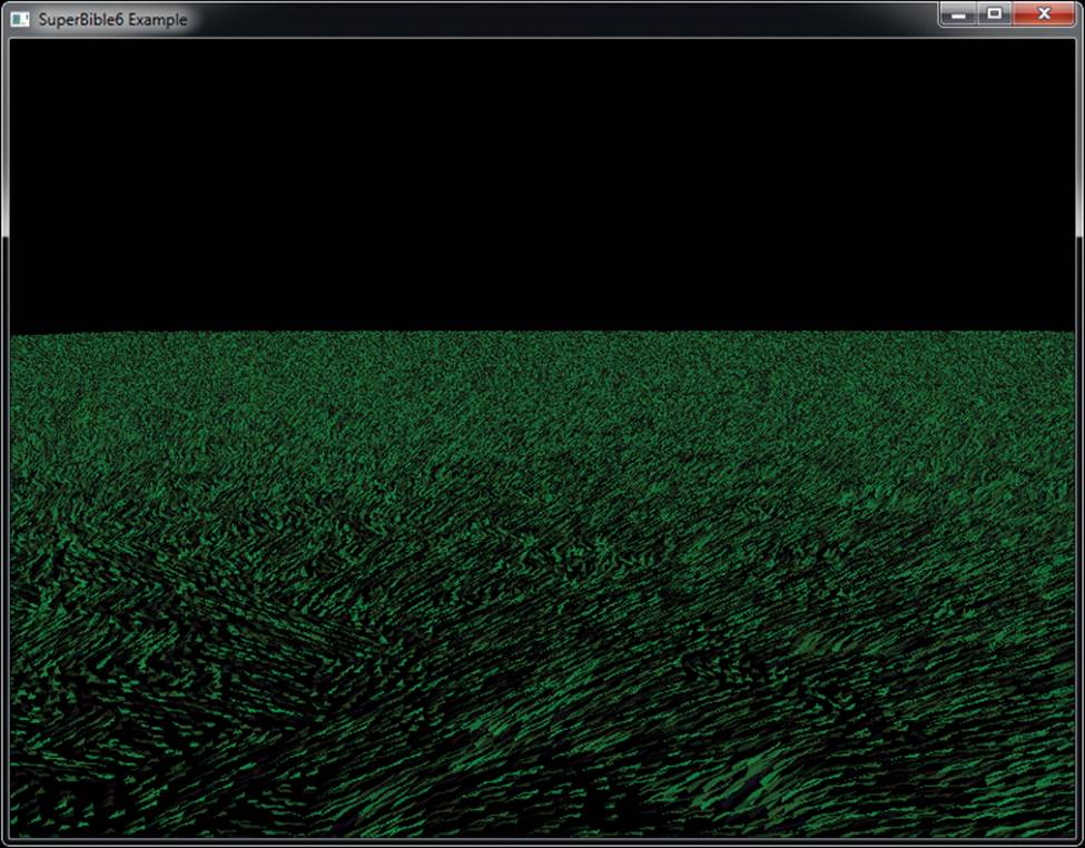
Figure 7.7: The final field of grass
Now, our final field has a million blades of grass, evenly distributed, with application control over length, “flatness,” direction of bend, or sway and color. Remember, the only input to the shader that differentiates one blade of grass from another is gl_InstanceID, the total amount of geometry sent to OpenGL is six vertices, and the total amount of code required to draw all the grass in the field is a single call to glDrawArraysInstanced().
The parameter texture can be read using linear texturing to provide smooth transitions between regions of grass and can be a fairly low resolution. If you want to make your grass wave in the wind or get trampled as hoards of armies march across it, you can animate the texture by updating it every frame or two and uploading a new version of it before you render the grass. Also, because the gl_InstanceID is used to generate random numbers, adding an offset to it before passing it to the random number generator allows a different but predetermined chunk of “random” grass to be generated with the same shader.
Getting Your Data Automatically
When you call one of the instanced drawing commands such as glDrawArraysInstanced() or glDrawElementsInstanced(), the built-in variable gl_InstanceID will be available in your shaders to tell you which instance you’re working on, and it will increment by one for each new instance of the geometry that you’re rendering. It’s actually available even when you’re not using one of the instanced drawing functions—it’ll just be zero in those cases. This means that you can use the same shaders for instanced and non-instanced rendering.
You can use gl_InstanceID to index into arrays that are the same length as the number of instances that you’re rendering. For example, you can use it to look up texels in a texture or to index into a uniform array. Really, what you’d be doing though is treating the array as if it were an “instanced attribute.” That is, a new value of the attribute is read for each instance you’re rendering. OpenGL can feed this data to your shader automatically using a feature called instanced arrays. To use instanced arrays, declare an input to your shader as normal. The input attribute will have an index that you would use in calls to functions like glVertexAttribPointer(). Normally, the vertex attributes would be read per vertex and a new value would be fed to the shader. However, to make OpenGL read attributes from the arrays once per instance, you can call
void glVertexAttribDivisor(GLuint index,
GLuint divisor);
Pass the index of the attribute to the function in index and set divisor to the number of instances you’d like to pass between each new value being read from the array. If divisor is zero, then the array becomes a regular vertex attribute array with a new value read per vertex. If divisor is non-zero, however, then new data is read from the array once every divisor instances. For example, if you set divisor to one, you’ll get a new value from the array for each instance. If you set divisor to two, you’ll get a new value for every second instance, and so on. You can mix and match the divisors, setting different values for each attribute. An example of using this functionality would be when you want to draw a set of objects with different colors. Consider the simple vertex shader in Listing 7.7.
#version 430 core
in vec4 position;
in vec4 color;
out Fragment
{
vec4 color;
} fragment;
uniform mat4 mvp;
void main(void)
{
gl_Position = mvp * position;
fragment.color = color;
}
Listing 7.7: Simple vertex shader with per-vertex color
Normally, the attribute color would be read once per vertex, and so every vertex would end up having a different color. The application would have to supply an array of colors with as many elements as there were vertices in the model. Also, it wouldn’t be possible for every instance of the object to have a different color because the shader doesn’t know anything about instancing. We can make color an instanced array if we call
glVertexAttribDivisor(index_of_color, 1);
where index_of_color is the index of the slot to which the color attribute has been bound. Now, a new value of color will be fetched from the vertex array once per instance. Every vertex within any particular instance will receive the same value for color, and the result will be that each instance of the object will be rendered in a different color. The size of the vertex array holding the data for color only needs to be as long as the number of indices we want to render. If we increase the value of the divisor, new data will be read from the array with less and less frequency. If the divisor is two, a new value of color will be presented every second instance; if the divisor is three, color will be updated every third instance; and so on. If we render geometry using this simple shader, each instance will be drawn on top of the others. We need to modify the position of each instance so that we can see each one. We can use another instanced array for this. Listing 7.8 shows a simple modification to the vertex shader in Listing 7.7.
#version 430 core
in vec4 position;
in vec4 instance_color;
in vec4 instance_position;
out Fragment
{
vec4 color;
} fragment;
uniform mat4 mvp;
void main(void)
{
gl_Position = mvp * (position + instance_position);
fragment.color = instance_color;
}
Listing 7.8: Simple instanced vertex shader
Now, we have a per-instance position as well as a per-vertex position. We can add these together in the vertex shader before multiplying with the model-view-projection matrix. We can set the instance_position input attribute to an instanced array by calling
glVertexAttribDivisor(index_of_instance_position, 1);
Again, index_of_instance_position is the index of the location to which the instance_position attribute has been bound. Any type of input attribute can be made instanced using glVertexAttribDivisor. This example is simple and only uses a translation (the value held in instance_position). A more advanced application could use matrix vertex attributes or pack some transformation matrices into uniforms and pass matrix weights in instanced arrays. The application can use this to render an army of soldiers, each with a different pose, or a fleet of spaceships all flying in different directions.
Now let’s hook this simple shader up to a real program. First, we load our shaders as normal before linking the program. The vertex shader is shown in Listing 7.8, the fragment shader simply passes the color input to its output, and the application code to hook all this up is shown in Listing 7.9. In the code, we declare some data and load it into a buffer and attach it to a vertex array object. Some of the data is used as per-vertex positions, but the rest is used as per-instance colors and positions.
static const GLfloat square_vertices[] =
{
-1.0f, -1.0f, 0.0f, 1.0f,
1.0f, -1.0f, 0.0f, 1.0f,
1.0f, 1.0f, 0.0f, 1.0f,
-1.0f, 1.0f, 0.0f, 1.0f
};
static const GLfloat instance_colors[] =
{
1.0f, 0.0f, 0.0f, 1.0f,
0.0f, 1.0f, 0.0f, 1.0f,
0.0f, 0.0f, 1.0f, 1.0f,
1.0f, 1.0f, 0.0f, 1.0f
};
static const GLfloat instance_positions[] =
{
-2.0f, -2.0f, 0.0f, 0.0f,
2.0f, -2.0f, 0.0f, 0.0f,
2.0f, 2.0f, 0.0f, 0.0f,
-2.0f, 2.0f, 0.0f, 0.0f
};
GLuint offset = 0;
glGenVertexArrays(1, &square_vao);
glGenBuffers(1, &square_vbo);
glBindVertexArray(square_vao);
glBindBuffer(GL_ARRAY_BUFFER, square_vbo);
glBufferData(GL_ARRAY_BUFFER,
sizeof(square_vertices) +
sizeof(instance_colors) +
sizeof(instance_positions), NULL, GL_STATIC_DRAW);
glBufferSubData(GL_ARRAY_BUFFER, offset,
sizeof(square_vertices),
square_vertices);
offset += sizeof(square_vertices);
glBufferSubData(GL_ARRAY_BUFFER, offset,
sizeof(instance_colors), instance_colors);
offset += sizeof(instance_colors);
glBufferSubData(GL_ARRAY_BUFFER, offset,
sizeof(instance_positions), instance_positions);
offset += sizeof(instance_positions);
glVertexAttribPointer(0, 4, GL_FLOAT, GL_FALSE, 0, 0);
glVertexAttribPointer(1, 4, GL_FLOAT, GL_FALSE, 0,
(GLvoid *)sizeof(square_vertices));
glVertexAttribPointer(2, 4, GL_FLOAT, GL_FALSE, 0,
(GLvoid *)(sizeof(square_vertices) +
sizeof(instance_colors)));
glEnableVertexAttribArray(0);
glEnableVertexAttribArray(1);
glEnableVertexAttribArray(2);
Listing 7.9: Getting ready for instanced rendering
Now all that remains is to set the vertex attrib divisors for the instance_color and instance_position attribute arrays:
glVertexAttribDivisor(1, 1);
glVertexAttribDivisor(2, 1);
Now we draw four instances of the geometry that we previously put into our buffer. Each instance consists of four vertices, each with its own position, which means that the same vertex in each instance has the same position. However, all of the vertices in a single instance see the same value of instance_color and instance_position, and a new value of each is presented to each instance. Our rendering loop looks like this:
static const GLfloat black[] = { 0.0f, 0.0f, 0.0f, 0.0f };
glClearBufferfv(GL_COLOR, 0, black);
glUseProgram(instancingProg);
glBindVertexArray(square_vao);
glDrawArraysInstanced(GL_TRIANGLE_FAN, 0, 4, 4);
What we get is shown in Figure 7.8. In the figure, you can see that four rectangles have been rendered. Each is at a different position, and each has a different color. This can be extended to thousands or even millions of instances, and modern graphics hardware should be able to handle this without any issue.
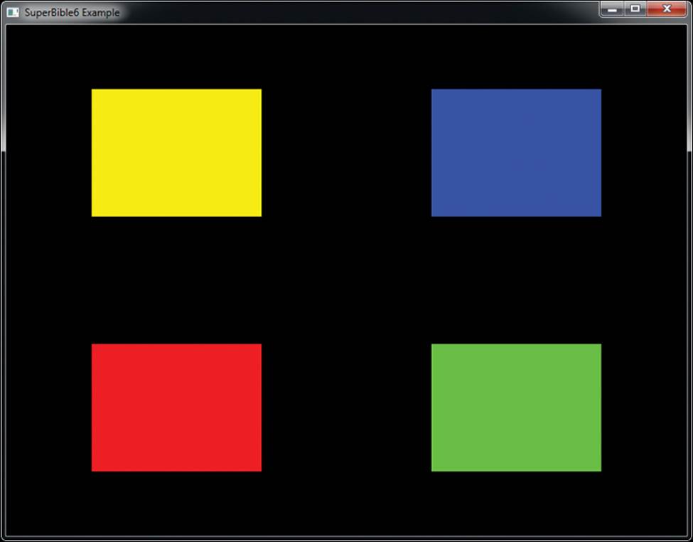
Figure 7.8: Result of instanced rendering
When you have instanced vertex attributes, you can use the baseInstance parameter to drawing commands such as glDrawArraysInstancedBaseInstance() to offset where in their respective buffers the data is read from. If you set this to zero (or call one of the functions that lacks this parameter), the data for the first instance comes from the start of the array. However, if you set it to a non-zero value, the index within the instanced array from which the data comes is offset by that value. This is very similar to the baseVertex parameter described earlier.
The actual formula for calculating the index from which attributes are fetched is
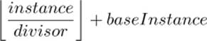
We will use the baseInstance parameter in some of the following examples to provide offsets into instanced vertex arrays.
Indirect Draws
So far, we have covered only direct drawing commands. In these commands, we pass the parameters of the draw such as the number of vertices or instances directly to the function. However, there is a family of drawing commands that allow the parameters of each draw to be stored in a buffer object. This means that at the time that your application calls the drawing command, it doesn’t actually need to know those parameters, only the location in the buffer where the parameters are stored. This opens a few interesting possibilities. For instance,
• Your application can generate the parameters for a drawing command ahead of time, possibly even offline, load them into a buffer, and then send them to OpenGL when it’s ready to draw.
• You can generate the parameters using OpenGL at runtime and store them in a buffer object from a shader, using them to render later parts of the scene.
There are four indirect drawing commands in OpenGL. The first two have direct equivalents; glDrawArraysIndirect() is the indirect equivalent to glDrawArraysInstancedBaseInstance(), and glDrawElementsIndirect() is equivalent toglDrawElementsInstancedBaseVertexBaseInstance(). The prototypes of these indirect functions are
void glDrawArraysIndirect(GLenum mode,
const void * indirect);
and
void glDrawElementsIndirect(GLenum mode,
GLenum type,
const void * indirect);
For both functions, mode is one of the primitive modes such as GL_TRIANGLES or GL_PATCHES. For glDrawElementsIndirect(), type is the type of the indices to be used (just like the type parameter to glDrawElements()) and should be set to GL_UNSIGNED_BYTE, GL_UNSIGNED_SHORT, orGL_UNSIGNED_INT. Again, for both functions, indirect is interpreted as an offset into the buffer object bound to the GL_DRAW_INDIRECT_BUFFER target, but the contents of the buffer at this address are different, depending on which function is being used. When expressed as a C-style structure definition, for glDrawArraysIndirect(), the form of the data in the buffer is
typedef struct {
GLuint vertexCount;
GLuint instanceCount;
GLuint firstVertex;
GLuint baseInstance;
} DrawArraysIndirectCommand;
For glDrawElementsIndirect(), the form of the data in the buffer is
typedef struct {
GLuint vertexCount;
GLuint instanceCount;
GLuint firstIndex;
GLint baseVertex;
GLuint baseInstance;
} DrawElementsIndirectCommand;
Calling glDrawArraysIndirect() will cause OpenGL to behave as if you had called glDrawArraysInstancedBaseInstance() with the mode you passed to glDrawArraysIndirect() but with the count, first, instancecount, and baseinstance parameters taken from the vertexCount,firstVertex, instanceCount, and baseInstance fields of the DrawArraysIndirectCommand structure stored in the buffer object at the offset given in the indirect parameter.
Likewise, calling glDrawElementsIndirect() will cause OpenGL to behave as if you had called glDrawElementsInstancedBaseVertexBaseInstance() with the mode and type parameters passed directly through, and with the count, instancecount, basevertex, and baseinstance parameters taken from the vertexCount, instanceCount, baseVertex, and baseInstance fields of the DrawElementsIndirectCommand structure in the buffer.
However, the one difference here is that the firstIndex parameter is in units of indices rather than bytes, and so is multiplied by the size of the index type to form the offset that would have been passed in the indices parameter to glDrawElements().
As handy as it may seem to be able to do this, what makes this feature particularly powerful is the multi versions of these two functions. These are
void glMultiDrawArraysIndirect(GLenum mode,
const void * indirect,
GLsizei drawcount,
GLsizei stride);
and
void glMultiDrawElementsIndirect(GLenum mode,
GLenum type,
const void * indirect,
GLsizei drawcount,
GLsizei stride);
These two functions behave very similarly to glDrawArraysIndirect() and glDrawElementsIndirect(). However, you have probably noticed two additional parameters to each of the functions. Both functions essentially perform the same operation as their non-multi variants in a loop on an array of DrawArraysIndirectCommand or DrawElementsIndirectCommand. structures. drawcount specifies the number of structures in the array, and stride specifies the number of bytes between the start of each of the structures in the buffer object. If stride is zero, then the arrays are considered to be tightly packed. Otherwise, it allows you to have structures with additional data in-between, and OpenGL will skip over that data as it traverses the array.
The practical upper limit on the number of drawing commands you can batch together using these functions really only depends on the amount of memory available to store them. The drawcount parameter can literally range to the billions, but with each command taking 16 or 20 bytes, a billion draw commands would consume 20 gigabytes of memory and probably take several seconds or even minutes to execute. However, it’s perfectly reasonable to batch together tens of thousands of draw commands into a single buffer. Given this, you can either preload a buffer object with the parameters for many draw commands, or generate a very large number of commands on the GPU. When you generate the parameters for your drawing commands using the GPU directly into the buffer object, you don’t need to wait for them to be ready before calling the indirect draw command that will consume them, and the parameters never make a round trip from the GPU to your application and back.
Listing 7.10 shows a simple example of how glMultiDrawArraysIndirect() might be used.
typedef struct {
GLuint vertexCount;
GLuint instanceCount;
GLuint firstVertex;
GLuint baseInstance;
} DrawArraysIndirectCommand;
DrawArraysIndirectCommand draws[] =
{
{
42, // Vertex count
1, // Instance count
0, // First vertex
0 // Base instance
},
{
192,
1,
327,
0,
},
{
99,
1,
901,
0
}
};
// Put "draws[]" into a buffer object
GLuint buffer;
glGenBuffers(1, &buffer);
glBindBuffer(GL_DRAW_INDIRECT_BUFFER, buffer);
glBufferData(GL_DRAW_INDIRECT_BUFFER, sizeof(draws),
draws, GL_STATIC_DRAW);
// This will produce 3 draws (the number of elements in draws[]), each
// drawing disjoint pieces of the bound vertex arrays
glMultiDrawArraysIndirect(GL_TRIANGLES,
NULL,
sizeof(draws) / sizeof(draws[0]),
0);
Listing 7.10: Example use of an indirect draw command
Simply batching together three drawing commands isn’t really that interesting, though. To show the real power of the indirect draw command, we’ll draw an asteroid field. This field will consist of 30,000 individual asteroids. First, we will take advantage of the sb6::object class’s ability to store multiple meshes within a single file. When such a file is loaded from disk, all of the vertex data is loaded into a single buffer object and associated with a single vertex array object. Each of the sub-objects has a starting vertex and a count of the number of vertices used to describe it. We can retrieve these from the object loader by calling sb6::object::get_sub_object_info(). The total number of sub-objects in the .sbm file is made available through the sb6::object::get_sub_object_count() function. Therefore, we can construct an indirect draw buffer for our asteroid field using the code shown in Listing 7.11.
object.load("media/objects/asteroids.sbm");
glGenBuffers(1, &indirect_draw_buffer);
glBindBuffer(GL_DRAW_INDIRECT_BUFFER, indirect_draw_buffer);
glBufferData(GL_DRAW_INDIRECT_BUFFER,
NUM_DRAWS * sizeof(DrawArraysIndirectCommand),
NULL,
GL_STATIC_DRAW);
DrawArraysIndirectCommand * cmd = (DrawArraysIndirectCommand *)
glMapBufferRange(GL_DRAW_INDIRECT_BUFFER,
0,
NUM_DRAWS * sizeof(DrawArraysIndirectCommand),
GL_MAP_WRITE_BIT | GL_MAP_INVALIDATE_BUFFER_BIT);
for (i = 0; i < NUM_DRAWS; i++)
{
object.get_sub_object_info(i % object.get_sub_object_count(),
cmd[i].first,
cmd[i].count);
cmd[i].primCount = 1;
cmd[i].baseInstance = i;
}
glUnmapBuffer(GL_DRAW_INDIRECT_BUFFER);
Listing 7.11: Setting up the indirect draw buffer for asteroids
Next, we need a way to communicate which asteroid we’re drawing to the vertex shader. There is no direct way to get this information from the indirect draw command into the shader. However, we can take advantage of the fact that all drawing commands are actually instanced drawing commands — commands that only draw a single copy of the object can be considered to draw a single instance. Therefore, we can set up an instanced vertex attribute, set the baseInstance field of the indirect drawing command structure to the index within that attribute’s array of the data that we wish to pass to the vertex shader, and then use that data for whatever we wish. You’ll notice that in Listing 7.11, we set the baseInstance field of each structure to the loop counter.
Next, we need to set up a corresponding input to our vertex shader. The input declaration for our asteroid field renderer is shown in Listing 7.12.
#version 430 core
layout (location = 0) in vec4 position;
layout (location = 1) in vec3 normal;
layout (location = 10) in uint draw_id;
Listing 7.12: Vertex shader inputs for asteroids
As usual, we have a position and normal input. However, we’ve also used an attribute at location 10, draw_id, to store our draw index. This attribute is going to be instanced and associated with a buffer that simply contains an identity mapping. We’re going to use the sb6::object loader’s functions to access and modify its vertex array object to inject our extra vertex attribute. The code to do this is shown in Listing 7.13.
glBindVertexArray(object.get_vao());
glGenBuffers(1, &draw_index_buffer);
glBindBuffer(GL_ARRAY_BUFFER, draw_index_buffer);
glBufferData(GL_ARRAY_BUFFER,
NUM_DRAWS * sizeof(GLuint),
NULL,
GL_STATIC_DRAW);
GLuint * draw_index =
(GLuint *)glMapBufferRange(GL_ARRAY_BUFFER,
0,
NUM_DRAWS * sizeof(GLuint),
GL_MAP_WRITE_BIT |
GL_MAP_INVALIDATE_BUFFER_BIT);
for (i = 0; i < NUM_DRAWS; i++)
{
draw_index[i] = i;
}
glUnmapBuffer(GL_ARRAY_BUFFER);
glVertexAttribIPointer(10, 1, GL_UNSIGNED_INT, 0, NULL);
glVertexAttribDivisor(10, 1);
glEnableVertexAttribArray(10);
Listing 7.13: Per-indirect draw attribute setup
Once we’ve set up our draw_id vertex shader input, we can use it to make each mesh unique. Without this, each asteroid would be a simple rock placed at the origin. In this example, we will directly create an orientation and translation matrix in the vertex shader from draw_id. The complete vertex shader is shown in Listing 7.14.
#version 430 core
layout (location = 0) in vec4 position;
layout (location = 1) in vec3 normal;
layout (location = 10) in uint draw_id;
out VS_OUT
{
vec3 normal;
vec4 color;
} vs_out;
uniform float time = 0.0;
uniform mat4 view_matrix;
uniform mat4 proj_matrix;
uniform mat4 viewproj_matrix;
const vec4 color0 = vec4(0.29, 0.21, 0.18, 1.0);
const vec4 color1 = vec4(0.58, 0.55, 0.51, 1.0);
void main(void)
{
mat4 m1;
mat4 m2;
mat4 m;
float t = time * 0.1;
float f = float(draw_id) / 30.0;
float st = sin(t * 0.5 + f * 5.0);
float ct = cos(t * 0.5 + f * 5.0);
float j = fract(f);
float d = cos(j * 3.14159);
// Rotate around Y
m[0] = vec4(ct, 0.0, st, 0.0);
m[1] = vec4(0.0, 1.0, 0.0, 0.0);
m[2] = vec4(-st, 0.0, ct, 0.0);
m[3] = vec4(0.0, 0.0, 0.0, 1.0);
// Translate in the XZ plane
m1[0] = vec4(1.0, 0.0, 0.0, 0.0);
m1[1] = vec4(0.0, 1.0, 0.0, 0.0);
m1[2] = vec4(0.0, 0.0, 1.0, 0.0);
m1[3] = vec4(260.0 + 30.0 * d, 5.0 * sin(f * 123.123), 0.0, 1.0);
m = m * m1;
// Rotate around X
st = sin(t * 2.1 * (600.0 + f) * 0.01);
ct = cos(t * 2.1 * (600.0 + f) * 0.01);
m1[0] = vec4(ct, st, 0.0, 0.0);
m1[1] = vec4(-st, ct, 0.0, 0.0);
m1[2] = vec4(0.0, 0.0, 1.0, 0.0);
m1[3] = vec4(0.0, 0.0, 0.0, 1.0);
m = m * m1;
// Rotate around Z
st = sin(t * 1.7 * (700.0 + f) * 0.01);
ct = cos(t * 1.7 * (700.0 + f) * 0.01);
m1[0] = vec4(1.0, 0.0, 0.0, 0.0);
m1[1] = vec4(0.0, ct, st, 0.0);
m1[2] = vec4(0.0, -st, ct, 0.0);
m1[3] = vec4(0.0, 0.0, 0.0, 1.0);
m = m * m1;
// Non-uniform scale
float f1 = 0.65 + cos(f * 1.1) * 0.2;
float f2 = 0.65 + cos(f * 1.1) * 0.2;
float f3 = 0.65 + cos(f * 1.3) * 0.2;
m1[0] = vec4(f1, 0.0, 0.0, 0.0);
m1[1] = vec4(0.0, f2, 0.0, 0.0);
m1[2] = vec4(0.0, 0.0, f3, 0.0);
m1[3] = vec4(0.0, 0.0, 0.0, 1.0);
m = m * m1;
gl_Position = viewproj_matrix * m * position;
vs_out.normal = mat3(view_matrix * m) * normal;
vs_out.color = mix(color0, color1, fract(j * 313.431));
}
Listing 7.14: Asteroid field vertex shader
In the vertex shader shown in Listing 7.14, we calculate the orientation, position, and color of the asteroid directly from draw_id. First, we convert draw_id to floating point and scale it. Next, we calculate a number of translation, scaling, and rotation matrices based on its value and the value of the time uniform. These matrices are concatenated to form a model matrix, m. The position is first transformed by the model matrix and then the view-projection matrix. The vertex’s normal is also transformed by the model and view matrices. Finally, an output color is computed for the vertex by interpolating between two colors (one is a chocolate brown, the other a sandy gray) to give the asteroid its final color. A simple lighting scheme is used in the fragment shader to give the asteroids a sense of depth.
The rendering loop for this application is extremely simple. First, we set up our view and projection matrices and then we render all of the models with a single call to glMultiDrawArraysIndirect(). The drawing code is shown in Listing 7.15.
glBindVertexArray(object.get_vao());
if (mode == MODE_MULTIDRAW)
{
glMultiDrawArraysIndirect(GL_TRIANGLES, NULL, NUM_DRAWS, 0);
}
else if (mode == MODE_SEPARATE_DRAWS)
{
for (j = 0; j < NUM_DRAWS; j++)
{
GLuint first, count;
object.get_sub_object_info(j % object.get_sub_object_count(),
first, count);
glDrawArraysInstancedBaseInstance(GL_TRIANGLES,
first,
count,
1, j);
}
}
Listing 7.15: Drawing asteroids
As you can see from Listing 7.15, we first bind the object’s vertex array object by calling object.get_vao() and passing the result to glBindVertexArray(). When mode is MODE_MULTIDRAW, the entire scene is drawn with a single call to glMultiDrawArraysIndirect(). However, if mode isMODE_SEPARATE_DRAWS, we loop over all of the loaded sub-objects and draw each separately by passing the same parameters that are loaded into the indirect draw buffer directly to a call to glDrawArraysInstancedBaseInstance(). Depending on your OpenGL implementation, the separate draw mode could be substantially slower. The resulting output is shown in Figure 7.9.
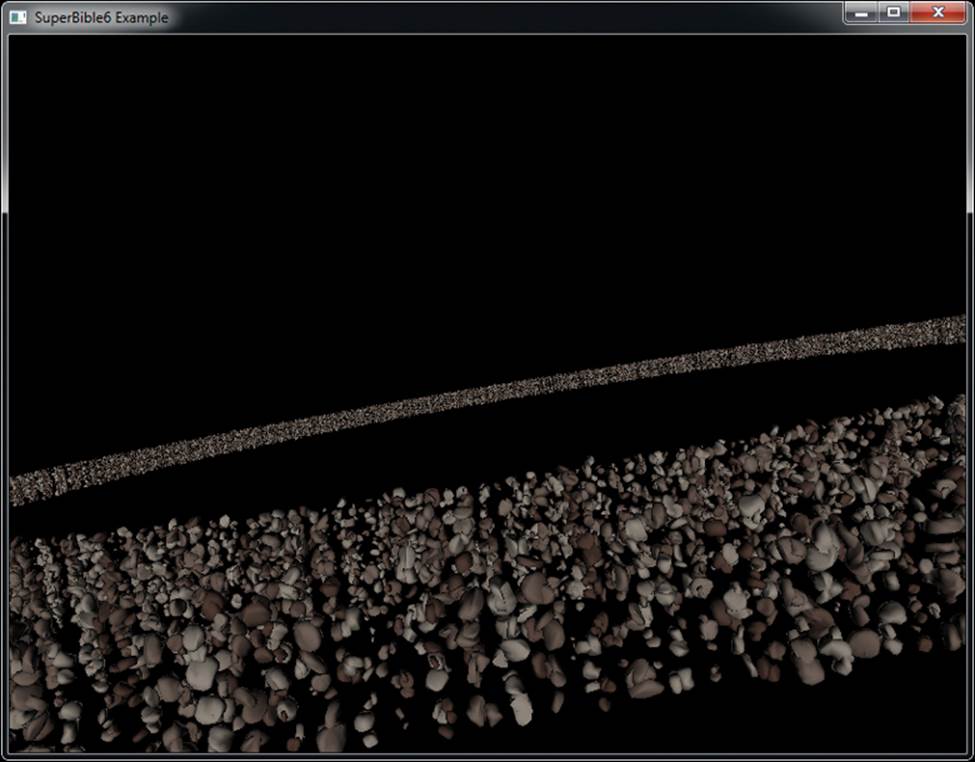
Figure 7.9: Result of asteroid rendering program
In our example, using a typical consumer graphics card, we can achieve 60 frames per second with 30,000 unique3 models, which is equivalent to 1.8 million drawing commands every second. Each mesh has approximately 500 vertices, which means that we’re rendering almost a billion vertices per second, and our bottleneck is almost certainly not the rate at which we are submitting drawing commands.
3. The asteroids in this example are not truly unique — they are selected from a large batch of unique rock models, and then a different scale and color are applied to each one. The chances of finding two rocks the same shape, at the same scale, and with the same color is vanishingly small.
With clever use of the draw_id input (or other instanced vertex attributes), more interesting geometry with more complex variation could be rendered. For example, we could use texture mapping to apply surface detail, storing a number of different surfaces in an array texture and selecting a layer using draw_id. There’s also no reason why the content of the indirect draw buffer need be static. In fact, we can generate its content directly on the graphics process using various techniques that will be explained shortly to achieve truly dynamic rendering without application intervention.
Storing Transformed Vertices
In OpenGL, it is possible to save the results of the vertex, tessellation evaluation, or geometry shader into one or more buffer objects. This is a feature known as transform feedback, and is effectively the last stage in the front end. It is a non-programmable, fixed-function stage in the OpenGL pipeline that is nonetheless highly configurable. When transform feedback is used, a specified set of attributes output from the last stage in the current shader pipeline (whether that be a vertex, tessellation evaluation, or geometry shader) are written into a set of buffers.
When no geometry shader is present, vertices processed by the vertex shader and perhaps tessellation evaluation shader are recorded. When a geometry shader is present, the vertices generated by the EmitVertex() function are stored, allowing a variable amount of data to be recorded depending on what the shader does. The buffers used for capturing the output of vertex and geometry shaders are known as transform feedback buffers. Once data has been placed into a buffer using transform feedback, it can be read back using a function like glGetBufferSubData() or by mapping it into the application’s address space using glMapBuffer() and reading from it directly. It can also be used as the source of data for subsequent drawing commands. For the remainder of this section, we will refer to the last stage in the front end as the vertex shader. However, be aware that if a geometry or tessellation evaluation shader is present, the last stage is the one whose outputs are saved by transform feedback.
Using Transform Feedback
To set up transform feedback, we must tell OpenGL which of the outputs from the front end we want to record. The outputs from the last stage of the front end are sometimes referred to as varyings. The function to tell OpenGL which ones to record is glTransformFeedbackVaryings(), and its prototype is
void glTransformFeedbackVaryings(GLuint program,
GLsizei count,
const GLchar * const * varying,
GLenum bufferMode);
The first parameter to glTransformFeedbackVaryings() is the name of a program object. The transform feedback varying state is actually maintained as part of a program object. This means that different programs can record different sets of vertex attributes, even if the same vertex or geometry shaders are used in them. The second parameter is the number of outputs (or varyings) to record and is also the length of the array whose address is given in the third parameter, varying. This third parameter is simply an array of C-style strings giving the names of the varyings to record. These are the names of the out variables in the vertex shader. Finally, the last parameter (bufferMode) specifies the mode in which the varyings are to be recorded. This must be either GL_SEPARATE_ATTRIBS or GL_INTERLEAVED_ATTRIBS. If bufferMode is GL_INTERLEAVED_ATTRIBS, the varyings are recorded into a single buffer, one after another. If bufferMode is GL_SEPARATE_ATTRIBS, each of the varyings is recorded into its own buffer. Consider the following piece of vertex shader code, which declares the output varyings:
out vec4 vs_position_out;
out vec4 vs_color_out;
out vec3 vs_normal_out;
out vec3 vs_binormal_out;
out vec3 vs_tangent_out;
To specify that the varyings vs_position_out, vs_color_out, and so on should be written into a single interleaved transform feedback buffer, the following C code could be used in your application:
static const char * varying_names[] =
{
"vs_position_out",
"vs_color_out",
"vs_normal_out",
"vs_binormal_out",
"vs_tangent_out"
};
const int num_varyings = sizeof(varying_names) /
sizeof(varying_names[0]);
glTransformFeedbackVaryings(program,
num_varyings,
varying_names,
GL_INTERLEAVED_ATTRIBS);
Not all of the outputs from your vertex (or geometry) shader need to be stored into the transform feedback buffer. It is possible to save a subset of the vertex shader outputs to the transform feedback buffer and send more to the fragment shader for interpolation. Likewise, it is also possible to save some outputs from the vertex shader into a transform feedback buffer that are not used by the fragment shader. Because of this, outputs from the vertex shader that may have been considered inactive (because they’re not used by the fragment shader) may become active due to their being stored in a transform feedback buffer. Therefore, after specifying a new set of transform feedback varyings by calling glTransformFeedbackVaryings(), it is necessary to link the program object using
glLinkProgram(program);
If you change the set of varyings captured by transform feedback, you need to link the program object again otherwise your changes won’t have any effect. Once the transform feedback varyings have been specified and the program has been linked, it may be used as normal. Before actually capturing anything, you need to create a buffer and bind it to an indexed transform feedback buffer binding point. Of course, before any data can be written to a buffer, space must be allocated in the buffer for it. To allocate space without specifying data, call
GLuint buffer;
glGenBuffers(1, &buffer);
glBindBuffer(GL_TARNSFORM_FEEDBACK_BUFFER, buffer);
glBufferData(GL_TRANSFORM_FEEDBACK_BUFFER, size, NULL, GL_DYNAMIC_COPY);
When you allocate storage for a buffer, there are many possible values for the usage parameter, but GL_DYNAMIC_COPY is probably a good choice for a transform feedback buffer. The DYNAMIC part tells OpenGL that the data is likely to change often but will likely be used a few times between each update. The COPY part says that you plan to update the data in the buffer through OpenGL functionality (such as transform feedback) and then hand that data back to OpenGL for use in another operation (such as drawing).
When you have specified the transform feedback mode as GL_INTERLEAVED_ATTRIBS, all of the stored vertex attributes are written one after another into a single buffer. To specify which buffer the transform feedback data will be written to, you need to bind a buffer to one of the indexed transform feedback binding points. There are actually multiple GL_TRANSFORM_FEEDBACK_BUFFER binding points for this purpose, which are conceptually separate but related to the general binding GL_TRANSFORM_FEEDBACK_BUFFER binding point. A schematic of this is shown in Figure 7.10.
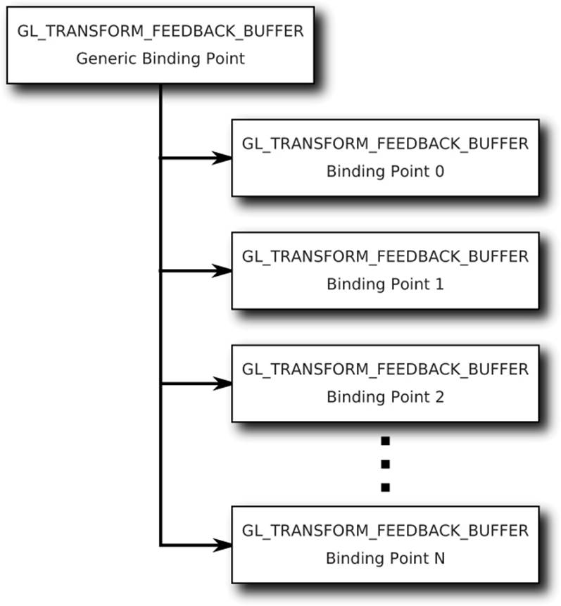
Figure 7.10: Relationship of transform feedback binding points
To bind a buffer to any of the indexed binding points, call
glBindBufferBase(GL_TRANSFORM_FEEDBACK_BUFFER, index, buffer);
As before, GL_TRANSFORM_FEEDBACK_BUFFER tells OpenGL that we’re binding a buffer object to store the results of transform feedback, and the last parameter, buffer, is the name of the buffer object we want to bind. The extra parameter, index, is the index of the GL_TRANSFORM_FEEDBACK_BUFFERbinding point. An important thing to note is that there is no way to directly address any of the extra binding points provided by glBindBufferBase() through functions like glBufferData() or glCopyBufferSubData(). However, when you call glBindBufferBase(), it actually binds the buffer to the indexed binding point and to the generic binding point. Therefore, you can use the extra binding points to allocate space in the buffer if you access the general binding point right after calling glBindBufferBase().
A slightly more advanced version of glBindBufferBase() is glBindBufferRange(), whose prototype is
void glBindBufferRange(GLenum target,
GLuint index,
GLuint buffer,
GLintptr offset,
GLsizeiptr size);
The glBindBufferRange() function allows you to bind a section of a buffer to an indexed binding point, whereas glBindBuffer() and glBindBufferBase() can only bind the whole buffer at once. The first three parameters (target, index, and buffer) have the same meanings as inglBindBufferBase(). The offset and size parameters are used to specify the start and length of the section of the buffer that you’d like to bind, respectively. You can even bind different sections of the same buffer to several different indexed binding points simultaneously. This enables you to use transform feedback in GL_SEPARATE_ATTRIBS mode to write each attribute of the output vertices into separate sections of a single buffer. If your application packs all attributes into a single vertex buffer and uses glVertexAttribPointer() to specify non-zero offsets into the buffer, this allows you to make the output of transform feedback match the input of your vertex shader.
If you specified that all of the attributes should be recorded into a single transform feedback buffer by using the GL_INTERLEAVED_ATTRIBS parameter to glTransformFeedbackVaryings(), the data will be tightly packed and written into the buffer bound to the first GL_TRANSFORM_FEEDBACK_BUFFERbinding point (that with index zero). However, if you specified that the mode for transform feedback is GL_SEPARATE_ATTRIBS, each output from the vertex shader will be recorded into its own separate buffer (or section of a buffer, if you used glBindBufferRange()). In this case, you need to bind multiple buffers or buffer sections as transform feedback buffers. The index parameter must be between zero and one less than the maximum number of varyings that can be recorded into separate buffers using transform feedback mode. This limit depends on your graphics hardware and drivers and can be found by calling glGetIntegerv() with the GL_MAX_TRANSFORM_FEEDBACK_SEPARATE_ATTRIBS parameter. This limit is also applied to the count parameter to glTransformFeedbackVaryings().
There is no fixed limit on the number of separate varyings that can be written to transform feedback buffers in GL_INTERLEAVED_ATTRIBS mode, but there is a maximum number of components that can be written into a buffer. For example, it is possible to write more vec3 varyings than vec4varyings into a buffer using transform feedback. Again, this limit depends on your graphics hardware and can be found using glGetIntegerv() with the GL_MAX_TRANSFORM_FEEDBACK_INTERLEAVED_COMPONENTS parameter.
If you need to, you can leave gaps in the output structures stored in the transform feedback buffer. When you do this, OpenGL will write a few elements, then skip some space in the output buffer, then write a few more components, and so on, leaving the unused space in the buffer unmodified. To do this you can include one of the “virtual” varying names, gl_SkipComponents1, gl_SkipComponents2, gl_SkipComponents3, or gl_SkipComponents4 to skip one, two, three, or four components’ worth of storage space in the output buffer.
Finally, it also possible to write one set of output varyings interleaved into one buffer while writing another set of attributes into another buffer. To do this, we use another special “virtual” varying name, gl_NextBuffer, which tells glTransformFeedbackVaryings() to move on to the next buffer binding index. When you use gl_NextBuffer, the bufferMode parameter must be GL_INTERLEAVED_ATTRIBS. As an example, consider the code
static const char * varying_names[] =
{
"carrots",
"peas",
"gl_NextBuffer",
"beans",
"potatoes"
};
const int num_varyings = sizeof(varying_names) / sizeof(varying_names[0]);
glTransformFeedbackVaryings(program,
num_varyings,
varying_names,
GL_INTERLEAVED_ATTRIBS);
After running this code and then calling glLinkProgram(), the transform feedback stage will be configured to write carrots and peas into the first of the transform feedback buffers and beans and potatoes to the second. You could even skip the first buffer binding altogether by setting the first varying name to gl_NextBuffer.
Starting, Pausing, and Stopping Transform Feedback
Once the buffers that are to receive the results of the transform feedback have been bound, transform feedback mode is activated by calling
void glBeginTransformFeedback(GLenum primitiveMode);
Now whenever vertices pass through OpenGL’s front end, output varyings from the last shader will be written to the transform feedback buffers. The parameter to the function, primitiveMode, tells OpenGL what types of geometry to expect. The acceptable parameters are GL_POINTS, GL_LINES, and GL_TRIANGLES. When you call glDrawArrays() or another OpenGL drawing function, the basic geometric type must match what you have specified as the transform feedback primitive mode, or you must have a geometry shader that outputs the appropriate primitive type. For example, ifprimitiveMode is GL_TRIANGLES, then the last stage of the front end must produce triangles. This means that if you have a geometry shader, it must output triangle_strip primitives, if you have a tessellation evaluation shader (and no geometry shader), its output mode must be triangles, and if you have neither, you must call glDrawArrays() with GL_TRIANGLES, GL_TRIANGLE_STRIP or GL_TRIANGLE_FAN. The mapping of transform feedback primitive mode to draw types is shown in Table 7.3.
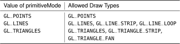
Table 7.3. Values for primitiveMode
In addition to the modes listed in Table 7.3, GL_PATCHES can be used for the drawing command’s mode parameter, so long as either the tessellation evaluation shader or geometry shader (if present) is configured to output the right type of primitives. Once transform feedback mode is activated, OpenGL will record your selected outputs from the front end into transform feedback buffers. You can temporarily suspend this recording by calling
void glPauseTransformFeedback();
When transform feedback mode is paused, it can be restarted again by calling
void glResumeTransformFeedback();
At this point, OpenGL will continue to record the output of the front end from wherever it left off in the transform feedback buffers. So long as transform feedback is not paused, vertices are recorded into the transform feedback buffers until transform feedback mode is exited or until the space allocated for the transform feedback buffers is exhausted. To exit transform feedback mode, call
glEndTransformFeedback();
All rendering that occurs between a call to glBeginTransformFeedback() and glEndTransformFeedback() results in data being written into the currently bound transform feedback buffers. Each time glBeginTransformFeedback() is called, OpenGL starts writing data at the beginning of the buffers bound for transform feedback, overwriting what might be there already. Some care should be taken while transform feedback is active as changing transform feedback state between calls to glBeginTransformFeedback() and glEndTransformFeedback() is not allowed. For example, it’s not possible to change the transform feedback buffer bindings or to resize or reallocate any of the transform feedback buffers while transform feedback mode is active. This includes cases where transform feedback is paused, even though it’s not recording during those times.
Ending the Pipeline with Transform Feedback
In many applications of transform feedback, it may well be that you simply want to store the vertices that the transform feedback stage produces, but you don’t actually want to draw anything. As transform feedback logically sits right before rasterization in the OpenGL pipeline, we can ask OpenGL to turn off rasterization (and therefore anything after it) by calling
glEnable(GL_RASTERIZER_DISCARD);
This stops OpenGL from processing primitives any further after transform feedback has been executed. The result is that our vertices are recorded into the output transform feedback buffers, but nothing is actually rasterized. To turn rasterization back on, we call
glDisable(GL_RASTERIZER_DISCARD);
This disables rasterizer discard, enabling rasterization.
Transform Feedback Example — Physical Simulation
In the springmass example, we build a physical simulation of a mesh of springs and masses. Each vertex represents a weight, connected to up to four neighbors by elastic tethers. The example iterates over the vertices, processing each one with a vertex shader. A number of advanced features are used in this example. We use a texture buffer object (TBO) to hold vertex position data in addition to a regular attribute array. The same buffer is bound to both the TBO and the vertex attribute associated with the position input to the vertex shader. This allows us to arbitrarily access the current position of other vertices in the system. We also use an integer vertex attribute to hold indices of neighboring vertices. Furthermore, we use transform feedback to store the positions and velocities of each of the masses between each iteration of the algorithm.
For each vertex, we need a position, velocity, and mass. We can pack the positions and masses into one vertex array and pack the velocities into another. Each element of the position array is actually a vec4, with the x, y, and z components containing the three-dimensional coordinate of the vertex, and the w component containing the weight of the vertex. The velocity array can simply be an array of vec3. Additionally, we use an array of ivec4 to store information about the springs connecting the weights together. There is one ivec4 for each vertex, and each of the four components of the vector contains the index of the vertex that is connected to the other end of the spring. We call this the connection vector. This means that we can connect each mass to up to four other masses. To record that there is no connection, we store a -1 in the corresponding component of the connection vector (see Figure 7.11).
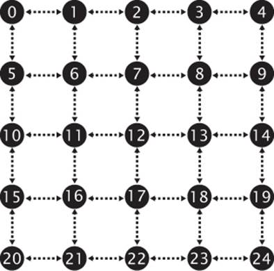
Figure 7.11: Connections of vertices in the spring-mass system
Consider vertex 12. It has associated with it an ivec4 connection vector containing <7, 13, 17, 11> — the indices of the vertices to which it is connected. Likewise, the connection vector for vertex 13 contains <8, 14, 18, 12>. There is a bidirectional connection between vertices 12 and 13. The vertices at the edges of the mesh don’t have all of their springs attached. So vertex 14 has a connection vector containing <9, -1, 19, 13>. Notice that the y component of the vector contains -1, indicating that there is no spring there.
Because for each of the connection vectors we either store the index of the vertex to which we are connected or -1 to indicate that no connection is present, we know that by storing a -1 in each of the connection vector components, we can fix that vertex in place. No matter what forces are acting on it, its position won’t be updated. This allows us to fix the position of some of the vertices and hold the structure in place. If all components of the connection vector are -1, then the calculations for updating the position and velocity of the vertex will be skipped by simply setting the force associated with that vertex to zero. The code to set up the initial positions and velocities of each node and the connection vectors for our spring-mass system is shown in Listing 7.16.
vmath::vec4 * initial_positions = new vmath::vec4 [POINTS_TOTAL];
vmath::vec3 * initial_velocities = new vmath::vec3 [POINTS_TOTAL];
vmath::ivec4 * connection_vectors = new vmath::ivec4 [POINTS_TOTAL];
int n = 0;
for (j = 0; j < POINTS_Y; j++)
{
float fj = (float)j / (float)POINTS_Y;
for (i = 0; i < POINTS_X; i++)
{
float fi = (float)i / (float)POINTS_X;
initial_positions[n] = vmath::vec4((fi - 0.5f) * (float)POINTS_X,
(fj - 0.5f) * (float)POINTS_Y,
0.6f * sinf(fi) * cosf(fj),
1.0f);
initial_velocities[n] = vmath::vec3(0.0f);
connection_vectors[n] = vmath::ivec4(-1);
if (j != (POINTS_Y - 1))
{
if (i != 0)
connection_vectors[n][0] = n - 1;
if (j != 0)
connection_vectors[n][1] = n - POINTS_X;
if (i != (POINTS_X - 1))
connection_vectors[n][2] = n + 1;
if (j != (POINTS_Y - 1))
connection_vectors[n][3] = n + POINTS_X;
}
n++;
}
}
glGenVertexArrays(2, m_vao);
glGenBuffers(5, m_vbo);
for (i = 0; i < 2; i++)
{
glBindVertexArray(m_vao[i]);
glBindBuffer(GL_ARRAY_BUFFER, m_vbo[POSITION_A + i]);
glBufferData(GL_ARRAY_BUFFER,
POINTS_TOTAL * sizeof(vmath::vec4),
initial_positions, GL_DYNAMIC_COPY);
glVertexAttribPointer(0, 4, GL_FLOAT, GL_FALSE, 0, NULL);
glEnableVertexAttribArray(0);
glBindBuffer(GL_ARRAY_BUFFER, m_vbo[VELOCITY_A + i]);
glBufferData(GL_ARRAY_BUFFER,
POINTS_TOTAL * sizeof(vmath::vec3),
initial_velocities, GL_DYNAMIC_COPY);
glVertexAttribPointer(1, 3, GL_FLOAT, GL_FALSE, 0, NULL);
glEnableVertexAttribArray(1);
glBindBuffer(GL_ARRAY_BUFFER, m_vbo[CONNECTION]);
glBufferData(GL_ARRAY_BUFFER,
POINTS_TOTAL * sizeof(vmath::ivec4),
connection_vectors, GL_STATIC_DRAW);
glVertexAttribIPointer(2, 4, GL_INT, 0, NULL);
glEnableVertexAttribArray(2);
}
delete [] connection_vectors;
delete [] initial_velocities;
delete [] initial_positions;
// Attach the buffers to a pair of TBOs.
glGenTextures(2, m_pos_tbo);
glBindTexture(GL_TEXTURE_BUFFER, m_pos_tbo[0]);
glTexBuffer(GL_TEXTURE_BUFFER, GL_RGBA32F, m_vbo[POSITION_A]);
glBindTexture(GL_TEXTURE_BUFFER, m_pos_tbo[1]);
glTexBuffer(GL_TEXTURE_BUFFER, GL_RGBA32F, m_vbo[POSITION_B]);
Listing 7.16: Spring-mass system vertex setup
To update the system, we run a vertex shader that obtains its own position and connection vector using regular vertex attributes. It then looks up the current positions of the vertices it’s connected to by indexing into the TBO using the elements of the connection vector (which is also a regular vertex attribute). The code for initializing the TBOs is also shown at the end of Listing 7.16.
For each connected vertex, the shader can calculate the distance to it and thus the extension of the virtual spring between them. From this, it can calculate the force exerted upon it by the spring, calculate the acceleration this produces given the mass of the vertex, and produce a new position and velocity vector to use in the next iteration. It sounds complex, but it’s not—it’s just Newtonian physics and Hooke’s law.
Hooke’s law is
F = –kx
where F is the force exerted by the spring, k is the spring constant (how stiff the spring is), and x is the extension of the spring. The spring’s extension is relative to its resting length. For our system, we keep the rest length of the springs the same and store it in a uniform. Any stretching of the spring produces a positive value of x, and any compression of the spring produces a negative value of x. The instantaneous length of the spring is simply the length of the vector from one of its ends to the other—exactly what we’ll calculate in the vertex shader. We give the force a direction by multiplying the linear force F by the direction along the spring. We introduce the variable ![]() , which is simply the normalized direction along the spring:
, which is simply the normalized direction along the spring:
![]()
This gives us the force applied to the mass due to the extension or compression of the spring. If we were to simply apply this force to the mass, the system would oscillate and, due to numerical imprecision, would eventually become unstable. All real spring systems have some loss due to friction, and this can be modeled by including damping into the force equation. The force due to damping is determined by the equation
![]()
where c represents the damping coefficient. Ideally, we would calculate the damping force for each spring, but for this simple system, a single force based on the mass’s velocity will do. Also, we use the initial velocity at each time-step to approximate the continuous differential that would be required by this equation. In our shader, we initialize F by calculating the damping force and then accumulate the force exerted by each spring on the mass. Finally, we can apply gravity to the system by treating it as simply one more force acting on each mass. Gravity is a constant force that generally acts in a downward direction. We can just add that to the initial force acting on the mass:
![]()
Once we have the total force, we can simply apply Newton’s laws. First, Newton’s second law allows us to calculate the acceleration of the mass:

Here, F is the force we just calculated using gravity, the damping coefficient, and Hooke’s law; m is the mass of the vertex (stored in the w component of the position attribute); and a is the resulting acceleration. Given the initial velocity (which we get from our other attribute array), we can plug it into the following equations of motion to find out what our final velocity will be and how far we moved in a fixed time:
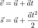
where u is the initial velocity (read from our velocity attribute array), v is the final velocity, t is our time-step (supplied by the application), and s is the distance we’ve travelled. Don’t forget, a, u, v, and s are all vectors. All that’s left to do is write the shaders and hook them up to an application. Listing 7.17 shows what the vertex shader looks like.
#version 430 core
// This input vector contains the vertex position in xyz, and the
// mass of the vertex in w
layout (location = 0) in vec4 position_mass;
// This is the current velocity of the vertex
layout (location = 1) in vec3 velocity;
// This is our connection vector
layout (location = 2) in ivec4 connection;
// This is a TBO that will be bound to the same buffer as the
// position_mass input attribute
layout (binding = 0) uniform samplerBuffer tex_position;
// The outputs of the vertex shader are the same as the inputs
out vec4 tf_position_mass;
out vec3 tf_velocity;
// A uniform to hold the time-step. The application can update this.
uniform float t = 0.07;
// The global spring constant
uniform float k = 7.1;
// Gravity
const vec3 gravity = vec3(0.0, -0.08, 0.0);
// Global damping constant
uniform float c = 2.8;
// Spring resting length
uniform float rest_length = 0.88;
void main(void)
{
vec3 p = position_mass.xyz; // p can be our position
float m = position_mass.w; // m is the mass of our vertex
vec3 u = velocity; // u is the initial velocity
vec3 F = gravity * m - c * u; // F is the force on the mass
bool fixed_node = true; // Becomes false when force is applied
for (int i = 0; i < 4; i++)
{
if (connection[i] != -1)
{
// q is the position of the other vertex
vec3 q = texelFetch(tex_position, connection[i]).xyz;
vec3 d = q - p;
float x = length(d);
F += -k * (rest_length - x) * normalize(d);
fixed_node = false;
}
}
// If this is a fixed node, reset force to zero
if (fixed_node)
{
F = vec3(0.0);
}
// Acceleration due to force
vec3 a = F / m;
// Displacement
vec3 s = u * t + 0.5 * a * t * t;
// Final velocity
vec3 v = u + a * t;
// Constrain the absolute value of the displacement per step
s = clamp(s, vec3(-25.0), vec3(25.0));
// Write the outputs
tf_position_mass = vec4(p + s, m);
tf_velocity = v;
}
Listing 7.17: Spring-mass system vertex shader
That wasn’t so hard, was it? To execute the shader, we iterate over our set of vertices that we placed in buffers earlier. We need to double-buffer the position and velocity information, which means that we read from one set of buffers and write to the other on one pass, and then swap the buffers around so that the data moves back and forth from one buffer to the other. The connection information remains the same on each pass, so it’s going to be constant. To do this, we use the two VAOs that we set up earlier. The first VAO has one set of position and velocity attributes attached to it, along with the common connection information. The other VAO has the other set of position and velocity attributes attached and the same, common connection information.
In addition to the VBOs, we need two TBOs. We use each buffer as a position VBO and as a TBO, simultaneously. This seems strange, but is perfectly legal in OpenGL—after all, we’re just reading from the same buffer via two different methods. To set this up, we generate two textures, bind them to the GL_TEXTURE_BUFFER binding point, and attach the buffers to them using glTexBuffer(), as explained earlier in this book. When we bind VAO A, we also bind texture A. When we bind VAO B, we bind texture B. That way, the same data appears in both the position vertex attribute and in the tex_position samplerBuffer buffer texture.
The code to set this up isn’t particularly complex but is repetitive. A complete implementation can be found on this book’s Web site. The example application includes the code to create and initialize the buffers, perform double buffering, and visualize the results. The application fixes a couple of the vertices in place so that the whole system doesn’t just fall off the bottom of the screen. Once we have all of the buffers hooked up, we can simulate a time-step in the system with a single call to glDrawArrays(). Each node in the system is represented by a single GL_POINTSprimitive. If we initialize the system and let it run, we see a result that looks like Figure 7.12.
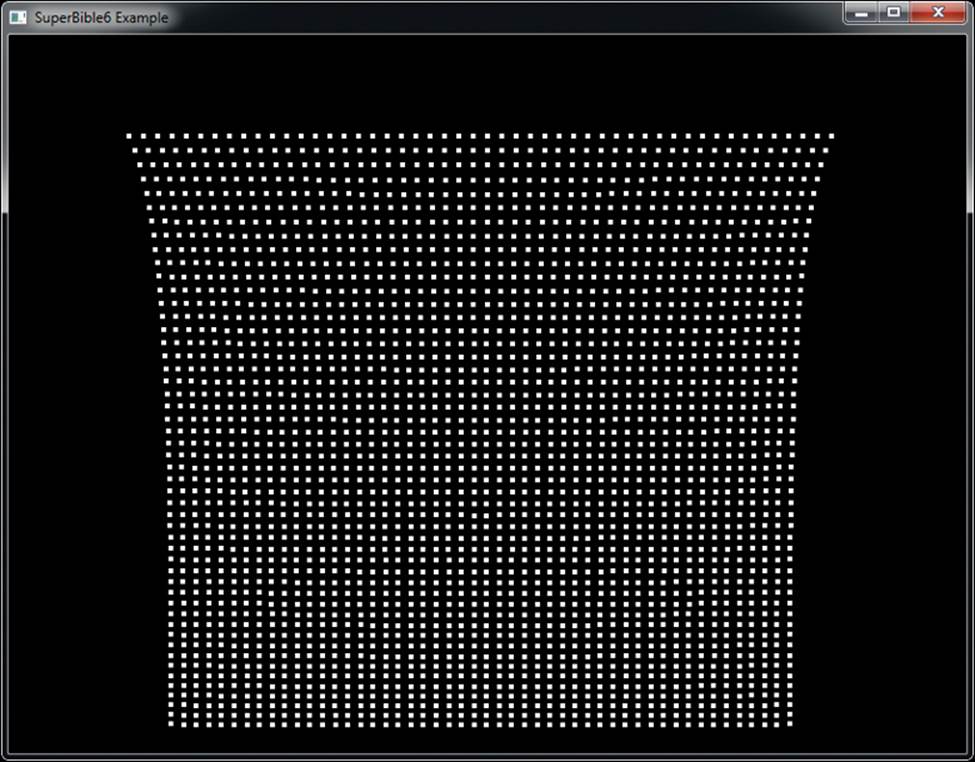
Figure 7.12: Simulation of points connected by springs
On each frame, we run the physical simulation several times, and on each iteration we swap the VAOs and TBOs. This iterative loop is shown in Listing 7.18. Each iteration of the loop updates the positions and velocities of all the nodes once. Iterating the simulation several times rather than just using a larger time-step in the simulation leads to greater stability and less oscillation of nodes, which leads to a better visual result.
int i;
glUseProgram(m_update_program);
glEnable(GL_RASTERIZER_DISCARD);
for (i = iterations_per_frame; i != 0; --i)
{
glBindVertexArray(m_vao[m_iteration_index & 1]);
glBindTexture(GL_TEXTURE_BUFFER, m_pos_tbo[m_iteration_index & 1]);
m_iteration_index++;
glBindBufferBase(GL_TRANSFORM_FEEDBACK_BUFFER, 0,
m_vbo[POSITION_A + (m_iteration_index & 1)]);
glBindBufferBase(GL_TRANSFORM_FEEDBACK_BUFFER, 1,
m_vbo[VELOCITY_A + (m_iteration_index & 1)]);
glBeginTransformFeedback(GL_POINTS);
glDrawArrays(GL_POINTS, 0, POINTS_TOTAL);
glEndTransformFeedback();
}
glDisable(GL_RASTERIZER_DISCARD);
Listing 7.18: Spring-mass system iteration loop
During iteration, we enable rasterizer discard, which stops data passing further down the pipeline beyond the transform feedback stage. We then disable rasterizer discard once we are done iterating so that we can render the resulting system to the screen. After enough iterations have been performed, we can render the points in the system in whatever way we wish. Using a simple program for rendering, we draw the nodes of the system as points and the connections between them as lines. Code to do this is shown in Listing 7.19, and the resulting image is shown in Figure 7.12.
static const GLfloat black[] = { 0.0f, 0.0f, 0.0f, 0.0f };
glViewport(0, 0, info.windowWidth, info.windowHeight);
glClearBufferfv(GL_COLOR, 0, black);
glUseProgram(m_render_program);
if (draw_points)
{
glPointSize(4.0f);
glDrawArrays(GL_POINTS, 0, POINTS_TOTAL);
}
if (draw_lines)
{
glBindBuffer(GL_ELEMENT_ARRAY_BUFFER, m_index_buffer);
glDrawElements(GL_LINES, CONNECTIONS_TOTAL * 2,
GL_UNSIGNED_INT, NULL);
}
Listing 7.19: Spring-mass system rendering loop
The image in Figure 7.12 is not particularly interesting, but it does demonstrate that our simulation is running correctly. To make the visual result more appealing, we can set the point size to a larger value, and we can also issue a second, indexed draw using glDrawElements() and GL_LINESprimitives to visualize the connections between nodes. Note that the same vertex positions can be used as input to this second pass, but we need to construct another buffer to use with the GL_ELEMENT_ARRAY binding that contains the indices of the vertices at the end of each spring. This additional step is also performed by the example program.
Figure 7.13 shows the final result.
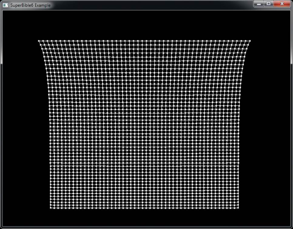
Figure 7.13: Visualizing springs in the spring-mass system
Of course, the physical simulation (and the vertex data produced by it) can be used for anything. This particular system would provide a reasonable approximation to cloth, although it is elementary. It does not, for instance, handle self-interaction, which would be important for a realistic cloth simulation. However, many systems in which particles interact in a deterministic way can be modeled and simulated using only a vertex shader and transform feedback.
Clipping
As explained in Chapter 3, “Following the Pipeline,” clipping is the process of determining which primitives may be fully or partially visible and constructing a set of primitives from them that will lie entirely inside the viewport.
For points, clipping is trivial — if the coordinate of the point is inside the region, then it should be processed further, whereas if it is outside the region it should be discarded. Clipping lines is a little more complex. If both ends of the line lie on the outside of the same plane of the clipping volume (for example, if the x component of both ends of the line is less than −1.0), then the line is trivially discarded. If both ends of the line lie inside the clipping volume, then it is trivially accepted. If one end of the line is inside the clipping volume or if the endpoints of the line lie such that it may cut through the clipping volume, then the line must be clipped against the volume to create a shorter line that lies within it. Figure 7.14 demonstrates trivially accepted, trivially discarded, and non-trivially clipped lines shown in two dimensions for clarity.
Figure 7.14: Clipping lines
In Figure 7.14 the line marked A is trivially accepted as both of its endpoints are entirely within the viewport (represented as a dotted rectangle). The line marked B is trivially rejected because both of its endpoints are outside the left edge of the viewport. Line C is clipped against the top edge of the viewport and line D is clipped against the left and bottom edges of the viewport. This is non-trivial clipping and results in vertices being moved along the line to make it fit into the viewport. Line E is a special case—the first endpoint is on the outside of the right edge of the viewport but the second is inside the right edge. However, the second endpoint of E is outside the bottom edge of the viewport whereas the first is inside that edge. OpenGL will still discard this line, but internally it may temporarily clip the line against one or other of the viewport edges before determining that there is nothing to be drawn.
The clipping of triangles poses a problem that appears to be more complex but is actually solved in a similar manner. As with lines, triangles may be trivially discarded if all three of their vertices lie on the outside of the same clipping plane and may be trivially accepted if all of their vertices lie inside the clipping volume. If the triangle lies partially inside and partially outside the clipping volume, then it must be clipped by cutting it into a number of smaller triangles that fit within the volume. Figure 7.15 demonstrates the process in two dimensions, although of course this really happens in three dimensions in OpenGL.
Figure 7.15: Clipping triangles
As you can see, the triangle marked A in Figure 7.15 is trivially accepted because all three of its vertices lie inside the viewport. Triangle B is trivially discarded because all three of its vertices lie outside of the same edge of the viewport. Triangle C crosses the left edge of the viewport and must be clipped. An additional vertex is generated by OpenGL, and the original triangle is split into two parts. Triangle D clips against the right and top edges of the viewport. An additional vertex is produced for each clipped edge, and new triangles are created to fill the polygonal shape that is produced. In fact, this is generally true — for each edge that a triangle clips, one extra vertex and one extra triangle are produced.
The Guard Band
As you can see in Figure 7.15, triangles that are partially visible but clip against one or more of the viewport edges can, depending on the implementation, be broken into multiple smaller triangles. This can cause a performance problem for GPUs that can process triangles at a fixed rate. In some cases, it may be faster to allow such triangles to pass through the clipping phase unmodified and instead have the rasterizer throw away parts that are not going to be visible. To implement this, some GPUs include a guard band, which is a region outside clip space in which triangles will be allowed to pass through even though they will not be visible. The guard band is illustrated in Figure 7.16.
Figure 7.16: Clipping triangles using a guard band
The presence of a guard band does not affect trivially accepted or trivially rejected triangles — those are either passed through or thrown away as they were before. However, triangles that clip against one or more edge of the viewport but otherwise fall inside the guard band are also considered to be trivially accepted and not are broken up. Only triangles that clip against one or more edges of the guard band and protrude into the viewport are broken into multiple triangles. Referring to Figure 7.16, we see that triangle A is trivially accepted as before and triangle B is trivially rejected as before. However, triangles C and D are no longer broken up. Rather, they are passed through the clipper unmodified and the shaded areas later discarded during rasterization. Only the newly introduced triangle E is broken into sub-triangles for rasterization. This is because it clips against both the viewport (the inner dotted rectangle) and the guard band (the outer dotted rectangle).
In practice, the width of the guard band (the gap between the inner and outer dotted rectangles) is quite large — usually at least as big as the viewport itself, and you’d have to draw some pretty huge triangles to hit both. While none of this will have any visible effect on the output of your program, it may affect its performance, and so is useful information.
User-Defined Clipping
One way to determine which side of a plane a point lies on is to calculate the signed distance from that point to the plane. When you know the signed distance from a point to a plane, its absolute value determines how far the point is to the plane, and its sign determines which side of the plane the point is on. Therefore, you can use the sign of this distance to determine whether you are inside or outside a plane. OpenGL may or may not use that method to perform view volume clipping, but you can use it to implement your own clipping algorithms.
In addition to the six distances to the six standard clip planes making up the view frustum, a set of additional distances is available to the application that can be written inside the vertex or geometry shader. The clip distances are available for writing in the vertex shader through the built-in variable gl_ClipDistance[], which is an array of floating-point values. As you learned earlier in this chapter, gl_ClipDistance[] is a member of the gl_PerVertex block and can be written from the vertex shader, tessellation evaluation, or geometry shader — whichever comes last. The number of clip distances supported depends on your implementation of OpenGL. These distances are interpreted exactly as the built-in clip distances. If a shader writer wants to use user-defined clip distances, they should be enabled by the application by calling
glEnable(GL_CLIP_DISTANCE0 + n);
Here, n is the index of the clip distance to enable. The tokens GL_CLIP_DISTANCE1, GL_CLIP_DISTANCE2, and so on up to GL_CLIP_DISTANCE5 are usually defined in standard OpenGL header files. However, the maximum value of n is implementation defined and can be found by callingglGetIntegerv() with the token GL_MAX_CLIP_DISTANCES. You can disable the user-defined clip distance by calling glDisable() with the same token. If the user-defined clip distance at a particular index is not enabled, the value written to gl_ClipDistance[] at that index is ignored.
As with the built-in clipping planes, the sign of the distance written into the gl_ClipDistance[] array is used to determine whether a vertex is inside or outside the user-defined clipping volume. If the signs of all the distances for every vertex of a single triangle are negative, the triangle is clipped. If it is determined that the triangle may be partially visible, then the clip distances are linearly interpolated across the triangle and the visibility determination is made at each pixel. Thus, the rendered result will be a linear approximation to the per-vertex distance function evaluated by the vertex shader. This allows a vertex shader to clip geometry against an arbitrary set of planes (the distance of a point to a plane can be found with a simple dot product).
The gl_ClipDistance[] array is also available as an input to the fragment shader. Fragments that would have a negative value in any element of gl_ClipDistance[] are clipped away and never reach the fragment shader. However, any fragment that only has positive values in gl_ClipDistance[]passes through the fragment shader, and this value can then be read and used by the shader for any purpose. One example use of this functionality is to fade the fragment by reducing its alpha value based as its clip distance approaches zero. This allows a large primitive clipped against a plane by the vertex shader to fade smoothly or be antialiased by the fragment shader, rather than generating a hard clipped edge.
Note that if all of the vertices making up a single primitive (point, line, or triangle) are clipped against the same plane, then the whole primitive is eliminated. This seems to make sense and behaves as expected for regular polygon meshes. However, when using points and lines, you need to be careful. With points, you can render a point with a single vertex that covers multiple pixels by setting the gl_PointSize parameter to a value greater than 1.0. When gl_PointSize is large, a big point is rendered around the vertex. This means that if you have a large point that is moving slowly toward and eventually off the edge of the screen, it will suddenly disappear when the center of the point exits the view volume and the vertex representing that point is clipped. Likewise, OpenGL can render wide lines. If a line is drawn whose vertices are both outside one of the clipping planes but would otherwise be visible, nothing will be drawn. This can produce strange popping artifacts if you’re not careful.
Listing 7.20 illustrates how a vertex shader might write to two clip distances. For the first clip distance, we determine the distance of the object-space vertex to a plane defined by the four-component vector, clip_plane. For the second distance, we consider the distance from each vertex to a sphere. To do this, we take the length of the vector from the view space vertex to the center of the sphere and subtract the sphere’s radius (which is stored in the w component of the clip_sphere).
#version 430 core
// More uniforms here
// Clip plane
uniform vec4 clip_plane = vec4(1.0, 1.0, 0.0, 0.85);
uniform vec4 clip_sphere = vec4(0.0, 0.0, 0.0, 4.0);
void main(void)
{
// Lighting code goes here
// Write clip distances
gl_ClipDistance[0] = dot(position, clip_plane);
gl_ClipDistance[1] = length(position.xyz / position.w -
clip_sphere.xyz) - clip_sphere.w;
// Calculate the clip-space position of each vertex
gl_Position = proj_matrix * P;
}
Listing 7.20: Clipping an object against a plane and a sphere
The result of rendering with the shader shown in Listing 7.20 is shown in Figure 7.17.
Figure 7.17: Rendering with user clip distances
As you can see in Figure 7.17, the dragon has not only been clipped against the flat plane, but also around the curved surface of the sphere. Be aware, though, that if the clip distance is linearly interpolated against a curved surface such as a sphere, the resulting clipped geometry will be a linear approximation to that curve. For good results, then, the original geometry must be reasonably detailed.
Summary
This chapter covered in some detail the mechanisms by which OpenGL reads vertex data from the buffers that you provide and how you map the inputs to your vertex shader to those inputs. We’ve also discussed the responsibilities of the vertex shader and the built-in output variables that it can write. You have seen how the vertex shader can not only set the resulting position of the vertices that it produces, but also the size for any points that might be rendered, and even how it can control the clipping process to allow you to clip objects against arbitrary shapes.
You have been introduced to transform feedback — a powerful stage in OpenGL that allows the vertex shader to store arbitrary data into buffers. We have looked at how OpenGL clips the primitives it generates against the visible region of the window and how primitives are moved from clip space into not just a single viewport, but into many viewports. In the next chapter, we’ll take another look at the front-end stages of tessellation and geometry shaders, which operate somewhat similarly to vertex shaders and will leverage the knowledge you’ve gained in this chapter.