Functional Programming in Scala (2015)
Part 1. Introduction to functional programming
Chapter 3. Functional data structures
We said in the introduction that functional programs don’t update variables or modify mutable data structures. This raises pressing questions: what sort of data structures can we use in functional programming, how do we define them in Scala, and how do we operate on them? In this chapter, we’ll learn the concept of functional data structures and how to work with them. We’ll use this as an opportunity to introduce how data types are defined in functional programming, learn about the related technique of pattern matching, and get practice writing and generalizing pure functions.
This chapter has a lot of exercises, particularly to help with this last point—writing and generalizing pure functions. Some of these exercises may be challenging. As always, consult the hints or the answers at our GitHub site (https://github.com/fpinscala/fpinscala; see the preface), or ask for help online if you need to.
3.1. Defining functional data structures
A functional data structure is (not surprisingly) operated on using only pure functions. Remember, a pure function must not change data in place or perform other side effects. Therefore, functional data structures are by definition immutable. For example, the empty list (written List() orNil in Scala) is as eternal and immutable as the integer values 3 or 4. And just as evaluating 3 + 4 results in a new number 7 without modifying either 3 or 4, concatenating two lists together (the syntax for this is a ++ b for two lists a and b) yields a new list and leaves the two inputs unmodified.
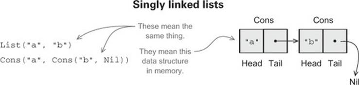
Doesn’t this mean we end up doing a lot of extra copying of the data? Perhaps surprisingly, the answer is no, and we’ll talk about exactly why that is. But first let’s examine what’s probably the most ubiquitous functional data structure, the singly linked list. The definition here is identical in spirit to (though simpler than) the List data type defined in Scala’s standard library. This code listing introduces a lot of new syntax and concepts that we’ll talk through in detail.
Listing 3.1. Singly linked lists
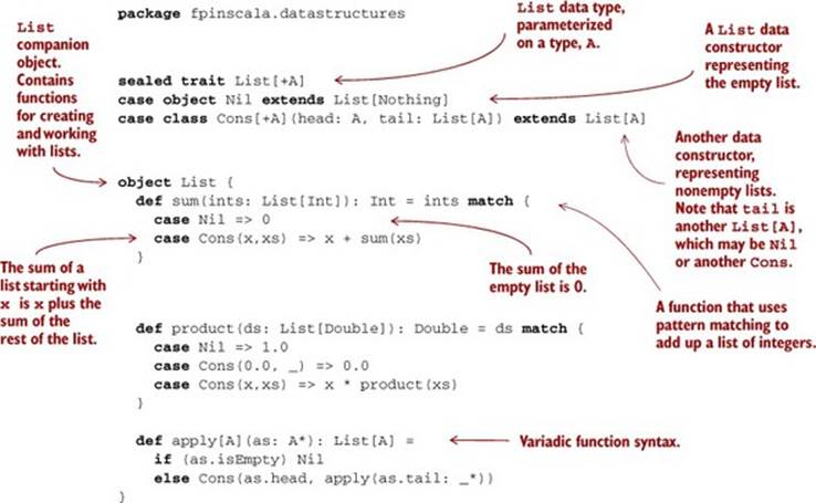
Let’s look first at the definition of the data type, which begins with the keywords sealed trait. In general, we introduce a data type with the trait keyword. A trait is an abstract interface that may optionally contain implementations of some methods. Here we’re declaring a trait, called List, with no methods on it. Adding sealed in front means that all implementations of the trait must be declared in this file.[1]
1 We could also say abstract class here instead of trait. The distinction between the two is not at all significant for our purposes right now. See section 5.3 in the Scala Language Specification (http://mng.bz/R75t) for more on the distinction.
There are two such implementations, or data constructors, of List (each introduced with the keyword case) declared next, to represent the two possible forms a List can take. As the figure at the top of page 31 shows, a List can be empty, denoted by the data constructor Nil, or it can be nonempty, denoted by the data constructor Cons (traditionally short for construct). A nonempty list consists of an initial element, head, followed by a List (possibly empty) of remaining elements (the tail):
case object Nil extends List[Nothing]
case class Cons[+A](head: A, tail: List[A]) extends List[A]
Just as functions can be polymorphic, data types can be as well, and by adding the type parameter [+A] after sealed trait List and then using that A parameter inside of the Cons data constructor, we declare the List data type to be polymorphic in the type of elements it contains, which means we can use this same definition for a list of Int elements (denoted List[Int]), Double elements (denoted List[Double]), String elements (List[String]), and so on (the + indicates that the type parameter A is covariant—see sidebar “More about variance” for more information).
A data constructor declaration gives us a function to construct that form of the data type. Here are a few examples:
val ex1: List[Double] = Nil
val ex2: List[Int] = Cons(1, Nil)
val ex3: List[String] = Cons("a", Cons("b", Nil))
The case object Nil lets us write Nil to construct an empty List, and the case class Cons lets us write Cons(1, Nil), Cons("a", Cons("b", Nil)) and so on to build singly linked lists of arbitrary lengths.[2] Note that because List is parameterized on a type, A, these are polymorphic functions that can be instantiated with different types for A. Here, ex2 instantiates the A type parameter to Int, while ex3 instantiates it to String. The ex1 example is interesting—Nil is being instantiated with type List[Double], which is allowed because the empty list contains no elements and can be considered a list of whatever type we want!
2 Scala generates a default def toString: String method for any case class or case object, which can be convenient for debugging. You can see the output of this default toString implementation if you experiment with List values in the REPL, which uses toString to render the result of each expression. Cons(1,Nil) will be printed as the string "Cons(1, Nil)", for instance. But note that the generated toString will be naively recursive and will cause stack overflow when printing long lists, so you may wish to provide a different implementation.
Each data constructor also introduces a pattern that can be used for pattern matching, as in the functions sum and product. We’ll examine pattern matching in more detail next.
More about variance
In the declaration trait List[+A], the + in front of the type parameter A is a variance annotation that signals that A is a covariant or “positive” parameter of List. This means that, for instance, List[Dog] is considered a subtype of List[Animal], assuming Dog is a subtype ofAnimal. (More generally, for all types X and Y, if X is a subtype of Y, then List[X] is a subtype of List[Y]). We could leave out the + in front of the A, which would make List invariant in that type parameter.
But notice now that Nil extends List[Nothing]. Nothing is a subtype of all types, which means that in conjunction with the variance annotation, Nil can be considered a List[Int], a List[Double], and so on, exactly as we want.
These concerns about variance aren’t very important for the present discussion and are more of an artifact of how Scala encodes data constructors via subtyping, so don’t worry if this is not completely clear right now. It’s certainly possible to write code without using variance annotations at all, and function signatures are sometimes simpler (whereas type inference often gets worse). We’ll use variance annotations throughout this book where it’s convenient to do so, but you should feel free to experiment with both approaches.
3.2. Pattern matching
Let’s look in detail at the functions sum and product, which we place in the object List, sometimes called the companion object to List (see sidebar). Both these definitions make use of pattern matching:
def sum(ints: List[Int]): Int = ints match {
case Nil => 0
case Cons(x,xs) => x + sum(xs)
}
def product(ds: List[Double]): Double = ds match {
case Nil => 1.0
case Cons(0.0, _) => 0.0
case Cons(x,xs) => x * product(xs)
}
As you might expect, the sum function states that the sum of an empty list is 0, and the sum of a nonempty list is the first element, x, plus the sum of the remaining elements, xs.[3] Likewise the product definition states that the product of an empty list is 1.0, the product of any list starting with 0.0 is 0.0, and the product of any other nonempty list is the first element multiplied by the product of the remaining elements. Note that these are recursive definitions, which are common when writing functions that operate over recursive data types like List (which refers to itself recursively in its Cons data constructor).
3 We could call x and xs anything there, but it’s a common convention to use xs, ys, as, or bs as variable names for a sequence of some sort, and x, y, z, a, or b as the name for a single element of a sequence. Another common naming convention is h for the first element of a list (the head of the list), t for the remaining elements (the tail), and l for an entire list.
Pattern matching works a bit like a fancy switch statement that may descend into the structure of the expression it examines and extract subexpressions of that structure. It’s introduced with an expression (the target or scrutinee) like ds, followed by the keyword match, and a {}-wrapped sequence of cases. Each case in the match consists of a pattern (like Cons(x,xs)) to the left of the => and a result (like x * product(xs)) to the right of the =>. If the target matches the pattern in a case (discussed next), the result of that case becomes the result of the entire match expression. If multiple patterns match the target, Scala chooses the first matching case.
Companion objects in Scala
We’ll often declare a companion object in addition to our data type and its data constructors. This is just an object with the same name as the data type (in this case List) where we put various convenience functions for creating or working with values of the data type.
If, for instance, we wanted a function def fill[A](n: Int, a: A): List[A] that created a List with n copies of the element a, the List companion object would be a good place for it. Companion objects are more of a convention in Scala.[4] We could have called this module Foo if we wanted, but calling it List makes it clear that the module contains functions relevant to working with lists.
4 There is some special support for them in the language that isn’t really relevant for our purposes.
Let’s look at a few more examples of pattern matching:
· List(1,2,3) match { case _ => 42 } results in 42. Here we’re using a variable pattern, _, which matches any expression. We could say x or foo instead of _, but we usually use _ to indicate a variable whose value we ignore in the result of the case.[5]
5 The _ variable pattern is treated somewhat specially in that it may be mentioned multiple times in the pattern to ignore multiple parts of the target.
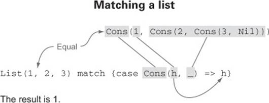
· List(1,2,3) match { case Cons(h,_) => h } results in 1. Here we’re using a data constructor pattern in conjunction with variables to capture or bind a subexpression of the target.
· List(1,2,3) match { case Cons(_,t) => t } results in List(2,3).
· List(1,2,3) match { case Nil => 42 } results in a MatchError at runtime. A MatchError indicates that none of the cases in a match expression matched the target.
What determines if a pattern matches an expression? A pattern may contain literals like 3 or "hi"; variables like x and xs, which match anything, indicated by an identifier starting with a lowercase letter or underscore; and data constructors like Cons(x,xs) and Nil, which match only values of the corresponding form. (Nil as a pattern matches only the value Nil, and Cons(h,t) or Cons(x,xs) as a pattern only match Cons values.) These components of a pattern may be nested arbitrarily—Cons(x1, Cons(x2, Nil)) and Cons(y1, Cons(y2, Cons(y3, _)))are valid patterns. A pattern matches the target if there exists an assignment of variables in the pattern to subexpressions of the target that make it structurally equivalent to the target. The resulting expression for a matching case will then have access to these variable assignments in its local scope.
Exercise 3.1
![]()
What will be the result of the following match expression?
val x = List(1,2,3,4,5) match {
case Cons(x, Cons(2, Cons(4, _))) => x
case Nil => 42
case Cons(x, Cons(y, Cons(3, Cons(4, _)))) => x + y
case Cons(h, t) => h + sum(t)
case _ => 101
}
You’re strongly encouraged to try experimenting with pattern matching in the REPL to get a sense for how it behaves.
Variadic functions in Scala
The function apply in the object List is a variadic function, meaning it accepts zero or more arguments of type A:
def apply[A](as: A*): List[A] =
if (as.isEmpty) Nil
else Cons(as.head, apply(as.tail: _*))
For data types, it’s a common idiom to have a variadic apply method in the companion object to conveniently construct instances of the data type. By calling this function apply and placing it in the companion object, we can invoke it with syntax like List(1,2,3,4) orList("hi","bye"), with as many values as we want separated by commas (we sometimes call this the list literal or just literal syntax).
Variadic functions are just providing a little syntactic sugar for creating and passing a Seq of elements explicitly. Seq is the interface in Scala’s collections library implemented by sequence-like data structures such as lists, queues, and vectors. Inside apply, the argument as will be bound to a Seq[A] (documentation at http://mng.bz/f4k9), which has the functions head (returns the first element) and tail (returns all elements but the first). The special _* type annotation allows us to pass a Seq to a variadic method.
3.3. Data sharing in functional data structures
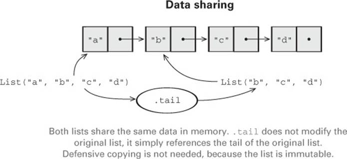
When data is immutable, how do we write functions that, for example, add or remove elements from a list? The answer is simple. When we add an element 1 to the front of an existing list, say xs, we return a new list, in this case Cons(1,xs). Since lists are immutable, we don’t need to actually copy xs; we can just reuse it. This is called data sharing. Sharing of immutable data often lets us implement functions more efficiently; we can always return immutable data structures without having to worry about subsequent code modifying our data. There’s no need to pessimistically make copies to avoid modification or corruption.[6]
6 Pessimistic copying can become a problem in large programs. When mutable data is passed through a chain of loosely coupled components, each component has to make its own copy of the data because other components might modify it. Immutable data is always safe to share, so we never have to make copies. We find that in the large, FP can often achieve greater efficiency than approaches that rely on side effects, due to much greater sharing of data and computation.
In the same way, to remove an element from the front of a list mylist = Cons(x,xs), we simply return its tail, xs. There’s no real removing going on. The original list, mylist, is still available, unharmed. We say that functional data structures are persistent, meaning that existing references are never changed by operations on the data structure.
Let’s try implementing a few different functions for modifying lists in different ways. You can place this, and other functions that we write, inside the List companion object.
Exercise 3.2
![]()
Implement the function tail for removing the first element of a List. Note that the function takes constant time. What are different choices you could make in your implementation if the List is Nil? We’ll return to this question in the next chapter.
Exercise 3.3
![]()
Using the same idea, implement the function setHead for replacing the first element of a List with a different value.
3.3.1. The efficiency of data sharing
Data sharing often lets us implement operations more efficiently. Let’s look at a few examples.
Exercise 3.4
![]()
Generalize tail to the function drop, which removes the first n elements from a list. Note that this function takes time proportional only to the number of elements being dropped—we don’t need to make a copy of the entire List.
def drop[A](l: List[A], n: Int): List[A]
Exercise 3.5
![]()
Implement dropWhile, which removes elements from the List prefix as long as they match a predicate.
def dropWhile[A](l: List[A], f: A => Boolean): List[A]
A more surprising example of data sharing is this function that adds all the elements of one list to the end of another:
def append[A](a1: List[A], a2: List[A]): List[A] =
a1 match {
case Nil => a2
case Cons(h,t) => Cons(h, append(t, a2))
}
Note that this definition only copies values until the first list is exhausted, so its runtime and memory usage are determined only by the length of a1. The remaining list then just points to a2. If we were to implement this same function for two arrays, we’d be forced to copy all the elements in both arrays into the result. In this case, the immutable linked list is much more efficient than an array!
Exercise 3.6
![]()
Not everything works out so nicely. Implement a function, init, that returns a List consisting of all but the last element of a List. So, given List(1,2,3,4), init will return List(1,2,3). Why can’t this function be implemented in constant time like tail?
def init[A](l: List[A]): List[A]
Because of the structure of a singly linked list, any time we want to replace the tail of a Cons, even if it’s the last Cons in the list, we must copy all the previous Cons objects. Writing purely functional data structures that support different operations efficiently is all about finding clever ways to exploit data sharing. We’re not going to cover these data structures here; for now, we’re content to use the functional data structures others have written. As an example of what’s possible, in the Scala standard library there’s a purely functional sequence implementation, Vector(documentation at http://mng.bz/Xhl8), with constant-time random access, updates, head, tail, init, and constant-time additions to either the front or rear of the sequence. See the chapter notes for links to further reading about how to design such data structures.
3.3.2. Improving type inference for higher-order functions
Higher-order functions like dropWhile will often be passed anonymous functions. Let’s look at a typical example.
Recall the signature of dropWhile:
def dropWhile[A](l: List[A], f: A => Boolean): List[A]
When we call it with an anonymous function for f, we have to specify the type of its argument, here named x:
val xs: List[Int] = List(1,2,3,4,5)
val ex1 = dropWhile(xs, (x: Int) => x < 4)
The value of ex1 is List(4,5).
It’s a little unfortunate that we need to state that the type of x is Int. The first argument to dropWhile is a List[Int], so the function in the second argument must accept an Int. Scala can infer this fact if we group dropWhile into two argument lists:
def dropWhile[A](as: List[A])(f: A => Boolean): List[A] =
as match {
case Cons(h,t) if f(h) => dropWhile(t)(f)
case _ => as
}
The syntax for calling this version of dropWhile looks like dropWhile(xs)(f). That is, dropWhile(xs) is returning a function, which we then call with the argument f (in other words, dropWhile is curried[7]). The main reason for grouping the arguments this way is to assist with type inference. We can now use dropWhile without annotations:
7 Recall from the previous chapter that a function of two arguments can be represented as a function that accepts one argument and returns another function of one argument.
val xs: List[Int] = List(1,2,3,4,5)
val ex1 = dropWhile(xs)(x => x < 4)
Note that x is not annotated with its type.
More generally, when a function definition contains multiple argument groups, type information flows from left to right across these argument groups. Here, the first argument group fixes the type parameter A of dropWhile to Int, so the annotation on x => x < 4 is not required.[8]
8 This is an unfortunate restriction of the Scala compiler; other functional languages like Haskell and OCaml provide complete inference, meaning type annotations are almost never required. See the notes for this chapter for more information and links to further reading.
We’ll often group and order our function arguments into multiple argument lists to maximize type inference.
3.4. Recursion over lists and generalizing to higher-order functions
Let’s look again at the implementations of sum and product. We’ve simplified the product implementation slightly, so as not to include the “short-circuiting” logic of checking for 0.0:
def sum(ints: List[Int]): Int = ints match {
case Nil => 0
case Cons(x,xs) => x + sum(xs)
}
def product(ds: List[Double]): Double = ds match {
case Nil => 1.0
case Cons(x, xs) => x * product(xs)
}
Note how similar these two definitions are. They’re operating on different types (List[Int] versus List[Double]), but aside from this, the only differences are the value to return in the case that the list is empty (0 in the case of sum, 1.0 in the case of product), and the operation to combine results (+ in the case of sum, * in the case of product). Whenever you encounter duplication like this, you can generalize it away by pulling subexpressions out into function arguments. If a subexpression refers to any local variables (the + operation refers to the local variables x andxs introduced by the pattern, similarly for product), turn the subexpression into a function that accepts these variables as arguments. Let’s do that now. Our function will take as arguments the value to return in the case of the empty list, and the function to add an element to the result in the case of a nonempty list.[9]
9 In the Scala standard library, foldRight is a method on List and its arguments are curried similarly for better type inference.
Listing 3.2. Right folds and simple uses
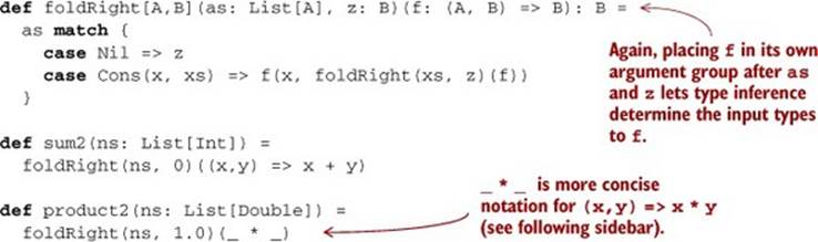
foldRight is not specific to any one type of element, and we discover while generalizing that the value that’s returned doesn’t have to be of the same type as the elements of the list! One way of describing what foldRight does is that it replaces the constructors of the list, Nil and Cons, with z and f, illustrated here:
Cons(1, Cons(2, Nil))
f (1, f (2, z ))
Let’s look at a complete example. We’ll trace the evaluation of foldRight(Cons(1, Cons(2, Cons(3, Nil))), 0)((x,y) => x + y) by repeatedly substituting the definition of foldRight for its usages. We’ll use program traces like this throughout this book:
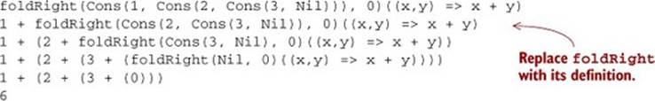
Note that foldRight must traverse all the way to the end of the list (pushing frames onto the call stack as it goes) before it can begin collapsing it.
Underscore notation for anonymous functions
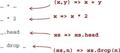
The anonymous function (x,y) => x + y can be written as _ + _ in situations where the types of x and y could be inferred by Scala. This is a useful shorthand in cases where the function parameters are mentioned just once in the body of the function. Each underscore in an anonymous function expression like _ + _ introduces a new (unnamed) function parameter and references it. Arguments are introduced in left-to-right order. Here are a few more examples:
Use this syntax judiciously. The meaning of this syntax in expressions like foo(_, g(List(_ + 1), _)) can be unclear. There are precise rules about scoping of these underscore-based anonymous functions in the Scala language specification, but if you have to think about it, we recommend just using ordinary named function parameters.
Exercise 3.7
![]()
Can product, implemented using foldRight, immediately halt the recursion and return 0.0 if it encounters a 0.0? Why or why not? Consider how any short-circuiting might work if you call foldRight with a large list. This is a deeper question that we’ll return to in chapter 5.
Exercise 3.8
![]()
See what happens when you pass Nil and Cons themselves to foldRight, like this: foldRight(List(1,2,3), Nil:List[Int])(Cons(_,_)).[10] What do you think this says about the relationship between foldRight and the data constructors of List?
10 The type annotation Nil:List[Int] is needed here, because otherwise Scala infers the B type parameter in foldRight as List[Nothing].
Exercise 3.9
![]()
Compute the length of a list using foldRight.
def length[A](as: List[A]): Int
Exercise 3.10
![]()
Our implementation of foldRight is not tail-recursive and will result in a StackOverflowError for large lists (we say it’s not stack-safe). Convince yourself that this is the case, and then write another general list-recursion function, foldLeft, that is tail-recursive, using the techniques we discussed in the previous chapter. Here is its signature:[11]
11 Again, foldLeft is defined as a method of List in the Scala standard library, and it is curried similarly for better type inference, so you can write mylist.foldLeft(0.0)(_ + _).
def foldLeft[A,B](as: List[A], z: B)(f: (B, A) => B): B
Exercise 3.11
![]()
Write sum, product, and a function to compute the length of a list using foldLeft.
Exercise 3.12
![]()
Write a function that returns the reverse of a list (given List(1,2,3) it returns List(3,2,1)). See if you can write it using a fold.
Exercise 3.13
![]()
Hard: Can you write foldLeft in terms of foldRight? How about the other way around? Implementing foldRight via foldLeft is useful because it lets us implement foldRight tail-recursively, which means it works even for large lists without overflowing the stack.
Exercise 3.14
![]()
Implement append in terms of either foldLeft or foldRight.
Exercise 3.15
![]()
Hard: Write a function that concatenates a list of lists into a single list. Its runtime should be linear in the total length of all lists. Try to use functions we have already defined.
3.4.1. More functions for working with lists
There are many more useful functions for working with lists. We’ll cover a few more here, to get additional practice with generalizing functions and to get some basic familiarity with common patterns when processing lists. After finishing this section, you’re not going to emerge with an automatic sense of when to use each of these functions. Just get in the habit of looking for possible ways to generalize any explicit recursive functions you write to process lists. If you do this, you’ll (re)discover these functions for yourself and develop an instinct for when you’d use each one.
Exercise 3.16
![]()
Write a function that transforms a list of integers by adding 1 to each element. (Reminder: this should be a pure function that returns a new List!)
Exercise 3.17
![]()
Write a function that turns each value in a List[Double] into a String. You can use the expression d.toString to convert some d: Double to a String.
Exercise 3.18
![]()
Write a function map that generalizes modifying each element in a list while maintaining the structure of the list. Here is its signature:[12]
12 In the standard library, map and flatMap are methods of List.
def map[A,B](as: List[A])(f: A => B): List[B]
Exercise 3.19
![]()
Write a function filter that removes elements from a list unless they satisfy a given predicate. Use it to remove all odd numbers from a List[Int].
def filter[A](as: List[A])(f: A => Boolean): List[A]
Exercise 3.20
![]()
Write a function flatMap that works like map except that the function given will return a list instead of a single result, and that list should be inserted into the final resulting list. Here is its signature:
def flatMap[A,B](as: List[A])(f: A => List[B]): List[B]
For instance, flatMap(List(1,2,3))(i => List(i,i)) should result in List(1,1,2,2,3,3).
Exercise 3.21
![]()
Use flatMap to implement filter.
Exercise 3.22
![]()
Write a function that accepts two lists and constructs a new list by adding corresponding elements. For example, List(1,2,3) and List(4,5,6) become List(5,7,9).
Exercise 3.23
![]()
Generalize the function you just wrote so that it’s not specific to integers or addition. Name your generalized function zipWith.
Lists in the Standard Library
List exists in the Scala standard library (API documentation at http://mng.bz/vu45), and we’ll use the standard library version in subsequent chapters. The main difference between the List developed here and the standard library version is that Cons is called ::, which associates to the right,[13] so 1 :: 2 :: Nil is equal to 1 :: (2 :: Nil), which is equal to List(1,2). When pattern matching, case Cons(h,t) becomes case h :: t, which avoids having to nest parentheses if writing a pattern like case h :: h2 :: t to extract more than just the first element of the List.
13 In Scala, all methods whose names end in : are right-associative. That is, the expression x :: xs is actually the method call xs.::(x), which in turn calls the data constructor ::(x,xs). See the Scala language specification for more information.
There are a number of other useful methods on the standard library lists. You may want to try experimenting with these and other methods in the REPL after reading the API documentation. These are defined as methods on List[A], rather than as standalone functions as we’ve done in this chapter:
· def take(n: Int): List[A] —Returns a list consisting of the first n elements of this
· def takeWhile(f: A => Boolean): List[A] —Returns a list consisting of the longest valid prefix of this whose elements all pass the predicate f
· def forall(f: A => Boolean): Boolean —Returns true if and only if all elements of this pass the predicate f
· def exists(f: A => Boolean): Boolean —Returns true if any element of this passes the predicate f
· scanLeft and scanRight—Like foldLeft and foldRight, but they return the List of partial results rather than just the final accumulated value
We recommend that you look through the Scala API documentation after finishing this chapter, to see what other functions there are. If you find yourself writing an explicit recursive function for doing some sort of list manipulation, check the List API to see if something like the function you need already exists.
3.4.2. Loss of efficiency when assembling list functions from simpler components
One of the problems with List is that, although we can often express operations and algorithms in terms of very general-purpose functions, the resulting implementation isn’t always efficient—we may end up making multiple passes over the same input, or else have to write explicit recursive loops to allow early termination.
Exercise 3.24
![]()
Hard: As an example, implement hasSubsequence for checking whether a List contains another List as a subsequence. For instance, List(1,2,3,4) would have List(1,2), List(2,3), and List(4) as subsequences, among others. You may have some difficulty finding a concise purely functional implementation that is also efficient. That’s okay. Implement the function however comes most naturally. We’ll return to this implementation in chapter 5 and hopefully improve on it. Note: Any two values x and y can be compared for equality in Scala using the expression x == y.
def hasSubsequence[A](sup: List[A], sub: List[A]): Boolean
3.5. Trees
List is just one example of what’s called an algebraic data type (ADT). (Somewhat confusingly, ADT is sometimes used elsewhere to stand for abstract data type.) An ADT is just a data type defined by one or more data constructors, each of which may contain zero or more arguments. We say that the data type is the sum or union of its data constructors, and each data constructor is the product of its arguments, hence the name algebraic data type.[14]
14 The naming is not coincidental. There’s a deep connection, beyond the scope of this book, between the “addition” and “multiplication” of types to form an ADT and addition and multiplication of numbers.
Tuple types in Scala
Pairs and tuples of other arities are also algebraic data types. They work just like the ADTs we’ve been writing here, but have special syntax:
scala> val p = ("Bob", 42)
p: (java.lang.String, Int) = (Bob,42)
scala> p._1
res0: java.lang.String = Bob
scala> p._2
res1: Int = 42
scala> p match { case (a,b) => b }
res2: Int = 42
In this example, ("Bob", 42) is a pair whose type is (String,Int), which is syntactic sugar for Tuple2[String,Int] (API link: http://mng.bz/1F2N). We can extract the first or second element of this pair (a Tuple3 will have a method _3, and so on), and we can pattern match on this pair much like any other case class. Higher arity tuples work similarly—try experimenting with them in the REPL if you’re interested.
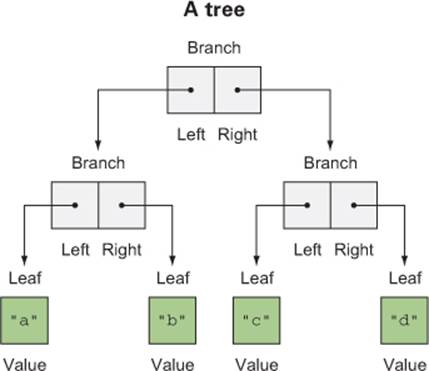
Algebraic data types can be used to define other data structures. Let’s define a simple binary tree data structure:
sealed trait Tree[+A]
case class Leaf[A](value: A) extends Tree[A]
case class Branch[A](left: Tree[A], right: Tree[A]) extends Tree[A]
Pattern matching again provides a convenient way of operating over elements of our ADT. Let’s try writing a few functions.
Exercise 3.25
![]()
Write a function size that counts the number of nodes (leaves and branches) in a tree.
Exercise 3.26
![]()
Write a function maximum that returns the maximum element in a Tree[Int]. (Note: In Scala, you can use x.max(y) or x max y to compute the maximum of two integers x and y.)
Exercise 3.27
![]()
Write a function depth that returns the maximum path length from the root of a tree to any leaf.
Exercise 3.28
![]()
Write a function map, analogous to the method of the same name on List, that modifies each element in a tree with a given function.
ADTs and encapsulation
One might object that algebraic data types violate encapsulation by making public the internal representation of a type. In FP, we approach concerns about encapsulation differently—we don’t typically have delicate mutable state which could lead to bugs or violation of invariants if exposed publicly. Exposing the data constructors of a type is often fine, and the decision to do so is approached much like any other decision about what the public API of a data type should be.[15]
15 It’s also possible in Scala to expose patterns like Nil and Cons independent of the actual data constructors of the type.
We do typically use ADTs for situations where the set of cases is closed (known to be fixed). For List and Tree, changing the set of data constructors would significantly change what these data types are. List is a singly linked list—that is its nature—and the two cases Nil and Cons form part of its useful public API. We can certainly write code that deals with a more abstract API than List (we’ll see examples of this later in the book), but this sort of information hiding can be handled as a separate layer rather than being baked into List directly.
Exercise 3.29
![]()
Generalize size, maximum, depth, and map, writing a new function fold that abstracts over their similarities. Reimplement them in terms of this more general function. Can you draw an analogy between this fold function and the left and right folds for List?
3.6. Summary
In this chapter, we covered a number of important concepts. We introduced algebraic data types and pattern matching, and showed how to implement purely functional data structures, including the singly linked list. We hope that, through the exercises in this chapter, you got more comfortable writing pure functions and generalizing them. We’ll continue to develop these skills in the chapters ahead.