Seven Concurrency Models in Seven Weeks (2014)
Chapter 8. The Lambda Architecture
If you need to ship freight in bulk from one side of the country to the other, nothing can beat a fleet of 18-wheeler trucks. But they’re not the right choice for delivering a single package, so an integrated shipping company also maintains a fleet of smaller cargo vans that perform local collections and deliveries.
The Lambda Architecture similarly combines the large-scale batch-processing strengths of MapReduce with the real-time responsiveness of stream processing to allow us to create scalable, responsive, and fault-tolerant solutions to Big Data problems.
Parallelism Enables Big Data
The advent of Big Data has brought about a sea change in data processing over recent years. Big Data differs from traditional data processing through its use of parallelism—only by bringing multiple computing resources to bear can we contemplate processing terabytes of data. The Lambda Architecture is a particular approach to Big Data popularized by Nathan Marz, derived from his time at BackType and subsequently Twitter.
Like last week’s topic, GPGPU programming, the Lambda Architecture leverages data parallelism. The difference is that it does so on a huge scale, distributing both data and computation over clusters of tens or hundreds of machines. Not only does this provide enough horsepower to make previously intractable problems tractable, but it also allows us to create systems that are fault tolerant against both hardware failure and human error.
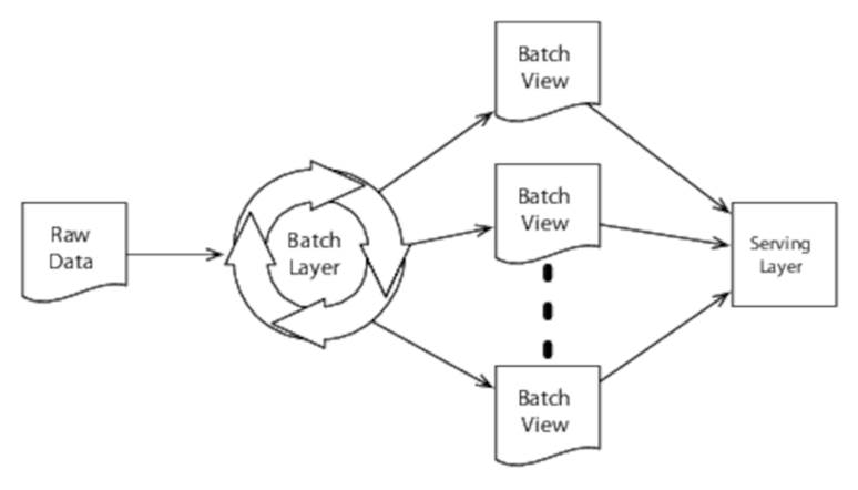
The Lambda Architecture has many facets. In this chapter we’re going to concentrate on its parallel and distributed aspects only (for a more complete discussion, see Nathan’s book, Big Data [MW14]). In particular, we’re going to concentrate on its two primary building blocks, the batch layer and the speed layer, as shown in Figure 18, The batch and speed layers.
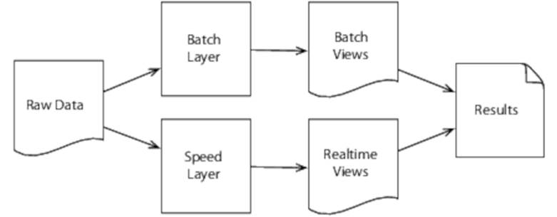
Figure 18. The batch and speed layers
The batch layer uses batch-oriented technologies like MapReduce to precompute batch views from historical data. This is effective, but latency is high, so we add a speed layer that uses low-latency techniques like stream processing to create real-time views from new data as it arrives. The two types of views are then combined to create query results.
The Lambda Architecture is by far the most complicated subject we’re going to cover in this book. It builds upon several underlying technologies, the most important of which is MapReduce. In day 1, therefore, we’ll concentrate solely upon MapReduce without worrying about how it fits into the wider picture. In day 2 we’ll look at the problems of traditional data systems and how MapReduce can solve them when used within the batch layer of the Lambda Architecture. Finally, in day 3 we’ll complete our picture of the Lambda Architecture by introducing stream processing and show how it can be used to construct the speed layer.
![]()
Joe asks:
Why the Name?
There’s been a lot of speculation about where the name comes from. I can do no better than quote the father of the Lambda Architecture, Nathan Marz:[55]
The name is due to the deep similarities between the architecture and functional programming. At the most fundamental level, the Lambda Architecture is a general way to compute functions on all your data at once.
Day 1: MapReduce
MapReduce is a broad term. Sometimes it’s used to describe the common pattern of breaking an algorithm down into two steps: a map over a data structure, followed by a reduce operation. Our functional word count (see the code) is an example of exactly this (remember that frequencies is implemented using reduce). As we saw in Day 2: Functional Parallelism, one of the benefits of breaking an algorithm down in this way is that it lends itself to parallelization.
But MapReduce can also be used to mean something more specific—a system that takes an algorithm encoded as a map followed by a reduce and efficiently distributes it across a cluster of computers. Not only does such a system automatically partition both the data and its processing between the machines within the cluster, but it also continues to operate if one or more of those machines fails.
MapReduce in this more specific sense was pioneered by Google.[56] Outside of Google, the most popular MapReduce framework is Hadoop.[57]
Today we’ll use Hadoop to create a parallel MapReduce version of the Wikipedia word-count example we’ve seen in previous chapters. Hadoop supports a wide variety of languages—we’re going to use Java.
Practicalities
Running Hadoop locally is very straightforward and is the normal starting point for developing and debugging a MapReduce job. Going beyond that to running on a cluster used to be difficult—not all of us have a pile of spare machines lying around, waiting to be turned into a cluster. And even if we did, installing, configuring, and maintaining a Hadoop cluster is notoriously time-consuming and involved.
Happily, cloud computing has dramatically improved matters by providing access to virtual servers on demand and by the hour. Even better, many providers now offer managed Hadoop clusters, dramatically simplifying configuration and maintenance.
In this chapter we’ll be using Amazon Elastic MapReduce, or EMR,[58] to run the examples. The means by which we start and stop clusters, and copy data to and from them, are specific to EMR, but the general principles apply to any Hadoop cluster.
To run the examples, you will need to have an Amazon AWS account with the AWS and EMR command-line tools installed.[59][60]
![]()
Joe asks:
What’s the Deal with Hadoop Releases?
Hadoop has a perversely confusing version-numbering scheme, with the 0.20.x, 1.x, 0.22.x, 0.23.x, 2.0.x, 2.1.x, and 2.2.x releases all in active use as I’m writing this. These releases support two different APIS, commonly known as the “old” (in the org.apache.hadoop.mapred package) and the “new” (in org.apache.hadoop.mapreduce), to varying degrees.
On top of this, various Hadoop distributions bundle a particular Hadoop release with a selection of third-party components.[61][62][63]
The examples in this chapter all use the new API and have been tested against Amazon’s 3.0.2 AMI, which uses Hadoop 2.2.0.[64]
Hadoop Basics
Hadoop is all about processing large amounts of data. Unless your data is measured in gigabytes or more, it’s unlikely to be the right tool for the job. Its power comes from the fact that that it splits data into sections, each of which is then processed independently by separate machines.
As you might expect, a MapReduce task is constructed from two primary types of components, mappers and reducers. Mappers take some input format (by default, lines of plain text) and map it to a number of key/value pairs. Reducers then convert these key/value pairs to the ultimate output format (normally also a set of key/value pairs). Mappers and reducers are distributed across many different physical machines (there’s no requirement for there to be the same number of mappers as reducers), as shown in Figure 19, Hadoop high-level data flow.
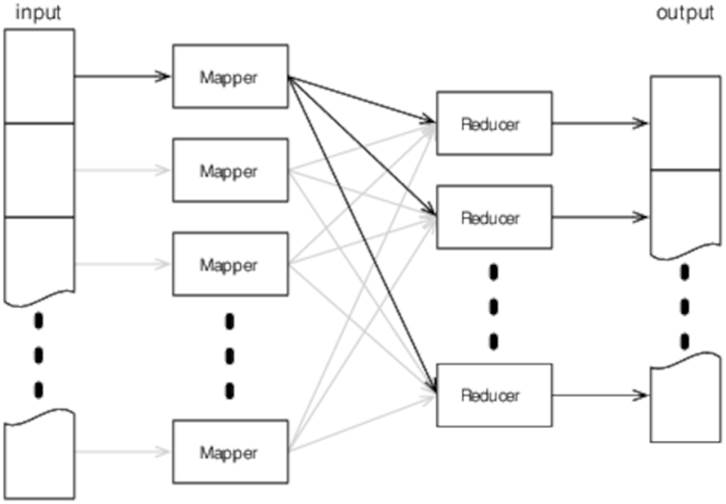
Figure 19. Hadoop high-level data flow
The input typically comprises one or more large text files. Hadoop splits these files (the size of each split depends on exactly how its configured, but a typical size would be 64 MB) and sends each split to a single mapper. The mapper outputs a number of key/value pairs, which Hadoop then sends to the reducers.
The key/value pairs from a single mapper are sent to multiple reducers. Which reducer receives a particular key/value pair is determined by the key—Hadoop guarantees that all pairs with the same key will be processed by the same reducer, no matter which mapper generated them. For obvious reasons, this is commonly called the shuffle phase.
Hadoop calls the reducer once for each key, with a list of all the values associated with it. The reducer combines these values and generates the final output (which is typically, but not necessarily, also key/value pairs).
So much for the theory—let’s see it in action by creating a Hadoop version of the Wikipedia word-count example we’ve already seen in previous chapters.
Counting Words with Hadoop
We’re going to start with a slightly simplified problem—counting the number of words in a collection of plain-text files (we’ll see how to extend this to counting the words in a Wikipedia XML dump soon).
Our mapper will process text a line at a time, break each line into words and output a single key/value pair for each word. The key will be the word itself, and the value will be the constant integer 1. Our reducer will take all the key/value pairs for a given word and sum the values, generating a single key/value pair for each word, where the value is a count of the number of times that word occurred in the input:
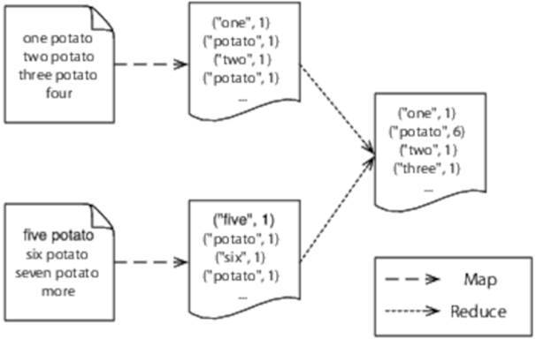
Figure 20. Counting words with Hadoop
The Mapper
Our mapper, Map, extends Hadoop’s Mapper class, which takes four type parameters—the input key type, the input value type, the output key type, and the output value type:
|
LambdaArchitecture/WordCount/src/main/java/com/paulbutcher/WordCount.java |
|
|
Line 1 |
public static class Map extends Mapper<Object, Text, Text, IntWritable> { |
|
- |
private final static IntWritable one = new IntWritable(1); |
|
- |
|
|
- |
public void map(Object key, Text value, Context context) |
|
5 |
throws IOException, InterruptedException { |
|
- |
|
|
- |
String line = value.toString(); |
|
- |
Iterable<String> words = new Words(line); |
|
- |
for (String word: words) |
|
10 |
context.write(new Text(word), one); |
|
- |
} |
|
- |
} |
Hadoop uses its own types to represent input and output data (we can’t use plain Strings and Integers). Our mapper handles plain text data, not key/value pairs, so the input key type is unused (we pass Object) and the input value type is Text. The output key type is also Text, with a value type of IntWritable.
The map method will be called once for each line of the input split. It starts by converting the line to a plain Java String (line 7) and then splits the String into words (line 8). Finally it iterates over those words, generating a single key/value pair for each of them, where the key is the word and the value the constant integer 1 (line 10).
The Reducer
Our reducer, Reduce, extends Hadoop’s Reducer class. Like Mapper, this also takes type parameters indicating the input and output key and value types (in our case, Text for both key types and IntWritable for both value types):
|
LambdaArchitecture/WordCount/src/main/java/com/paulbutcher/WordCount.java |
|
|
|
public static class Reduce extends Reducer<Text, IntWritable, Text, IntWritable> { |
|
|
public void reduce(Text key, Iterable<IntWritable> values, Context context) |
|
|
throws IOException, InterruptedException { |
|
|
int sum = 0; |
|
|
for (IntWritable val: values) |
|
|
sum += val.get(); |
|
|
context.write(key, new IntWritable(sum)); |
|
|
} |
|
|
} |
The reduce method will be called once for each key, with values containing a collection of all the values associated with that key. Our mapper simply sums the values and generates a single key/value pair associating the word with its total occurrences.
Now that we’ve got both our mapper and our reducer, our final task is to create a driver, which tells Hadoop how to run them.
The Driver
Our driver is a Hadoop Tool, which implements a run method:
|
LambdaArchitecture/WordCount/src/main/java/com/paulbutcher/WordCount.java |
|
|
Line 1 |
public class WordCount extends Configured implements Tool { |
|
- |
|
|
- |
public int run(String[] args) throws Exception { |
|
- |
Configuration conf = getConf(); |
|
5 |
Job job = Job.getInstance(conf, "wordcount"); |
|
- |
job.setJarByClass(WordCount.class); |
|
- |
job.setMapperClass(Map.class); |
|
- |
job.setReducerClass(Reduce.class); |
|
- |
job.setOutputKeyClass(Text.class); |
|
10 |
job.setOutputValueClass(IntWritable.class); |
|
- |
FileInputFormat.addInputPath(job, new Path(args[0])); |
|
- |
FileOutputFormat.setOutputPath(job, new Path(args[1])); |
|
- |
boolean success = job.waitForCompletion(true); |
|
- |
return success ? 0 : 1; |
|
15 |
} |
|
- |
|
|
- |
public static void main(String[] args) throws Exception { |
|
- |
int res = ToolRunner.run(new Configuration(), new WordCount(), args); |
|
- |
System.exit(res); |
|
20 |
} |
|
- |
} |
This is mostly boilerplate, simply informing Hadoop of what we’re doing. We set the mapper and reducer classes on lines 7 and 8, and the output key and value types on lines 9 and 10. We don’t need to set the input key and value type, because Hadoop assumes by default that we’re processing text files. And we don’t need to independently set the mapper output or reducer input key/value types, because Hadoop assumes by default that they’re the same as the output key/value types.
Next we tell Hadoop where to find the input data and where to write the output data on lines 11 and 12, and finally, we start the job and wait for it to complete on line 13.
Now that we’ve got a complete Hadoop job, all that remains is to run it on some data.
Running Locally
We’ll start by running locally. This won’t give us any of the benefits of parallelism or fault tolerance, but it does give us a way to check that everything’s working before the additional effort and expense of running on a full cluster.
First we’ll need some text to process. The input directory contains two text files comprising the literary masterpiece we’ll be analyzing:
|
LambdaArchitecture/WordCount/input/file1.txt |
|
|
|
one potato two potato three potato four |
|
LambdaArchitecture/WordCount/input/file2.txt |
|
|
|
five potato six potato seven potato more |
Not exactly gigabytes of data, to be sure, but there’s enough there to verify that the code works. We can count the text in these files by building with mvn package and then running a local instance of Hadoop with this:
|
|
$ hadoop jar target/wordcount-1.0-jar-with-dependencies.jar input output |
After Hadoop’s finished running, you should find that you have a new directory called output, which contains two files—_SUCCESS and part-r-00000. The first is an empty file that simply indicates that the job ran successfully. The second should contain the following:
|
|
five 1 |
|
|
four 1 |
|
|
more 1 |
|
|
one 1 |
|
|
potato 6 |
|
|
seven 1 |
|
|
six 1 |
|
|
three 1 |
|
|
two 1 |
Now that we’ve demonstrated that we can successfully run our job on a small file locally, we’re in a position to run it on a cluster and process much more data.
![]()
Joe asks:
Are Results Always Sorted?
You might have noticed that the results are sorted in (alphabetical) key order. Hadoop guarantees that keys will be sorted before being passed to a reducer, a fact that is very helpful for some tasks.
Be careful, however. Although the keys are sorted before they’re passed to each reducer, as we’ll see, by default there’s no ordering between reducers. This is something that can be controlled by setting a partitioner, but this isn’t something we’ll cover further here.
Running on Amazon EMR
Running a Hadoop job on Amazon Elastic MapReduce requires a number of steps. We won’t go into EMR in depth. But I do want to cover the steps in enough detail for you to be able to follow along.
Input and Output
By default, EMR takes its input from and writes its output to Amazon S3.[65] S3 is also the location of the JAR file containing the code to execute and where log files are written.
So to start, we’ll need an S3 bucket containing some plain-text files. A Wikipedia dump won’t do, because it’s XML, not plain text. The sample code for this chapter includes a project called ExtractWikiText that extracts the text from a Wikipedia dump, after which you can upload it to your S3 bucket. You’ll then need to upload the JAR file you built to another S3 bucket.
Uploading Large Files to S3
If, like me, your “broad”-band connection starts to wheeze when asked to upload large files, you might want to consider creating a short-lived Amazon EC2 instance with which to download the Wikipedia dump, extract the text from it, and upload it to S3. Unsurprisingly, Amazon provides excellent bandwidth between EC2 and S3, which can save your broadband’s blushes.
Creating a Cluster
You can create an EMR cluster in many different ways—we’re going to use the elastic-mapreduce command-line tool:
|
|
$ elastic-mapreduce --create --name wordcount --num-instances 11 \ |
|
|
--master-instance-type m1.large --slave-instance-type m1.large \ |
|
|
--ami-version 3.0.2 --jar s3://pb7con-lambda/wordcount.jar \ |
|
|
--arg s3://pb7con-wikipedia/text --arg s3://pb7con-wikipedia/counts |
|
|
Created job flow j-2LSRGPBSR79ZV |
This creates a cluster called “wordcount” with 11 instances, 1 master and 10 slaves, each of type m1.large running the 3.0.2 machine image (AMI).[66] The final arguments tell EMR where to find the JAR we uploaded to S3, where to find the input data, and where to put the results.
Monitoring Progress
We can use the job flow identifier returned when we created the cluster to establish an SSH connection to the master node:
|
|
$ elastic-mapreduce --jobflow j-2LSRGPBSR79ZV --ssh |
Now that we’ve got a command line on the master, we can monitor the progress of the job by looking at the log files:
|
|
$ tail -f /mnt/var/log/hadoop/steps/1/syslog |
|
|
INFO org.apache.hadoop.mapreduce.Job (main): map 0% reduce 0% |
|
|
INFO org.apache.hadoop.mapreduce.Job (main): map 1% reduce 0% |
|
|
INFO org.apache.hadoop.mapreduce.Job (main): map 2% reduce 0% |
|
|
INFO org.apache.hadoop.mapreduce.Job (main): map 3% reduce 0% |
|
|
INFO org.apache.hadoop.mapreduce.Job (main): map 4% reduce 0% |
Examining the Results
In my tests, this configuration takes a little over an hour to count all the words in Wikipedia. Once it’s finished, you should find a number of files in the S3 bucket you specified:
|
|
part-r-00000 |
|
|
part-r-00001 |
|
|
part-r-00002 |
|
|
⋮ |
|
|
part-r-00028 |
These files, taken in aggregate, contain the full set of results. Results are sorted within each result partition, but not across partitions (see Are Results Always Sorted?).
So we can now count words in plain-text files, but ideally we’d like to process a Wikipedia dump directly. We’ll look at how to do so next.
Processing XML
An XML file is, after all, just a text file with a little added structure, so you would be forgiven for thinking that we could process it in much the same way as we saw earlier. Doing so won’t work, however, because Hadoop’s default splitter divides files at line boundaries, meaning that it’s likely to split files in the middle of XML tags.
Although Hadoop doesn’t come with an XML-aware splitter as standard, it turns out that another Apache project, Mahout,[67] does provide one—XmlInputFormat.[68] To use it, we need to make a few small changes to our driver:
|
LambdaArchitecture/WordCountXml/src/main/java/com/paulbutcher/WordCount.java |
|
|
Line 1 |
public int run(String[] args) throws Exception { |
|
- |
Configuration conf = getConf(); |
|
- |
conf.set("xmlinput.start", "<text"); |
|
- |
conf.set("xmlinput.end", "</text>"); |
|
5 |
|
|
- |
Job job = Job.getInstance(conf, "wordcount"); |
|
- |
job.setJarByClass(WordCount.class); |
|
- |
job.setInputFormatClass(XmlInputFormat.class); |
|
- |
job.setMapperClass(Map.class); |
|
10 |
job.setCombinerClass(Reduce.class); |
|
- |
job.setReducerClass(Reduce.class); |
|
- |
job.setOutputKeyClass(Text.class); |
|
- |
job.setOutputValueClass(IntWritable.class); |
|
- |
FileInputFormat.addInputPath(job, new Path(args[0])); |
|
15 |
FileOutputFormat.setOutputPath(job, new Path(args[1])); |
|
- |
|
|
- |
boolean success = job.waitForCompletion(true); |
|
- |
return success ? 0 : 1; |
|
- |
} |
We’re using setInputFormatClass (line 8) to tell Hadoop to use XmlInputFormat instead of the default splitter and setting the xmlinput.start and xmlinput.end (lines 3 and 4) within the configuration to let the splitter know which tags we’re interested in.
If you look closely at the value we’re using for xmlinput.start, something might strike you as slightly odd—we’re setting it to <text, which isn’t a well-formed XML tag. XmlInputFormat doesn’t perform a full XML parse; instead it simply looks for start and end patterns. Because the <text>tag takes attributes, we just search for <text instead of <text>.
We also need to tweak our mapper slightly:
|
LambdaArchitecture/WordCountXml/src/main/java/com/paulbutcher/WordCount.java |
|
|
|
private final static Pattern textPattern = |
|
|
Pattern.compile("^<text.*>(.*)</text>$", Pattern.DOTALL); |
|
|
|
|
|
public void map(Object key, Text value, Context context) |
|
|
throws IOException, InterruptedException { |
|
|
|
|
|
String text = value.toString(); |
|
|
Matcher matcher = textPattern.matcher(text); |
|
|
if (matcher.find()) { |
|
|
Iterable<String> words = new Words(matcher.group(1)); |
|
|
for (String word: words) |
|
|
context.write(new Text(word), one); |
|
|
} |
|
|
} |
Each split consists of the text between the xmlinput.start and xmlinput.end patterns, including the matching patterns. So we use a little regular-expression magic to strip the <text><text> tags before counting words (to avoid overcounting the word text).
You may have noticed one other thing about our driver—we’re setting a combiner with setCombinerClass (line 10). A combiner is an optimization that allows key/value pairs to be combined before they’re sent to a reducer (see Figure 21, Using a combiner. In my tests, this decreases runtime from a little over an hour to around forty-five minutes.
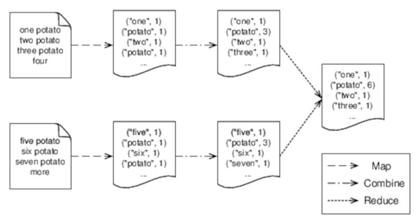
Figure 21. Using a combiner
In our case, our reducer works just as well as a combiner, but some algorithms will require a separate combiner. Hadoop does not guarantee use of a combiner if one is provided, so we need to make sure that our algorithm doesn’t depend on whether, or how often, it is used.
Day 1 Wrap-Up
That’s it for day 1. In day 2 we’ll see how to use Hadoop to construct the batch layer of the Lambda Architecture.
![]()
Joe asks:
Is It All About Speed?
It’s tempting to think that all Hadoop gives us is speed—allowing us to process large bodies of data more quickly than we could on a single machine, and certainly that’s a very important benefit. But there’s more to it than that:
· When we start talking about clusters of hundreds of machines, failure stops being a risk and becomes a likelihood. Any system that failed when one machine in the cluster failed would rapidly become unworkable. For that reason, Hadoop has been constructed from the ground up to be able to handle and recover from failure.
· Related to the preceding, we need to consider not only how to retry tasks that were in progress on a failed node, but also how to avoid loss of data if one or more discs fails. By default, Hadoop uses the Hadoop distributed file system (HDFS), a fault-tolerant distributed file system that replicates data across multiple nodes.
· Once we start talking about gigabytes or more of data, it becomes unreasonable to expect that we’ll be able to fit intermediate data or results in memory. Hadoop stores key/value pairs within HDFS during processing, allowing us to create jobs that process much larger datasets than will fit in memory.
Taken together, these aspects are transformative. It’s no coincidence that this chapter is the only one in which we’ve executed our Wikipedia word-count example on an entire Wikipedia dump—MapReduce is the only technology we’re going to cover that realistically allows that quantity of data to be processed.
What We Learned in Day 1
Breaking a problem into a map over a data structure followed by a reduce operation makes it easy to parallelize. MapReduce, in the sense we’re using the term in this chapter, specifically means a system that efficiently and fault-tolerantly distributes jobs constructed from maps and reduces over multiple machines. Hadoop is a MapReduce system that does the following:
· It splits input between a number of mappers, each of which generates key/value pairs.
· These are then sent to reducers, which generate the final output (typically also a set of key/value pairs).
· Keys are partitioned between reducers such that all pairs with the same key are handled by the same reducer.
Day 1 Self-Study
Find
· The documentation for Hadoop’s streaming API, which allows MapReduce jobs to be created in languages like Ruby, Python, or Perl
· The documentation for Hadoop’s pipes API, which allows MapReduce jobs to be created in C++
· A large number of libraries build on top of the Hadoop Java API to make it easier to construct more complex MapReduce jobs. For example, you might want to take a look at Cascading, Cascalog, or Scalding.
Do
· While a word-count job is running, kill one of the machines in the cluster (not the master—Hadoop is unable to recover if the master fails). Examine the logs while you do so to see how Hadoop retries the work that was assigned to that machine. Verify that the results are the same as for a job that doesn’t experience a failure.
· Our word-count program does what it claims, but it’s not very helpful if we want to answer the question “What are the top 100 most commonly used words on Wikipedia?” Implement a secondary sort (the Internet has many articles about how to do so) to generate fully sorted output from our word-count job.
· The “top-ten pattern” is an alternative way to solve the “most common words on Wikipedia” problem. Create a version of our word-count program that uses this pattern.
· Not all problems can be solved by a single MapReduce job—often it’s necessary to chain multiple jobs, with the output of one forming the input for the next. One example is the PageRank algorithm. Create a Hadoop program that calculates the page rank of each Wikipedia page. How many iterations does it take before the results stabilize?
Day 2: The Batch Layer
Yesterday we saw how we could use Hadoop to parallelize across a cluster of machines. MapReduce can be used to solve a huge range of problems, but today we’re going to concentrate on how it fits into the Lambda Architecture.
Before we look at that, however, let’s consider the problem that the Lambda Architecture exists to solve—what’s wrong with traditional data systems?
Problems with Traditional Data Systems
Data systems are nothing new—we’ve been using databases to answer questions about the data stored within them for almost as long as computers have existed. Traditional databases work well up to a point, but the volume of data we’re trying to handle these days is pushing them beyond the point where they can cope.
Scaling
Some techniques enable a traditional database to scale beyond a single machine (replication, sharding, and so on), but these become harder and harder to apply as the number of machines and the query volume grows. Beyond a certain point, adding machines simply doesn’t help.
Maintenance Overhead
Maintaining a database spread over a number of machines is hard. Doing so without downtime is even more so—if you need to reshard your database, for example. Then there’s fault tolerance, backup, and ensuring data integrity, all of which become exponentially more difficult as the volume of data and queries increases.
Complexity
Replication and sharding typically require support at the application layer—your application needs to know which replicas to query and which shards to update (which will typically vary from query to query in nonobvious ways). Often many of the facilities that programmers have grown used to, such as transaction support, disappear when a database is sharded, meaning that programmers have to handle failures and retries explicitly. All of this increases the chances of mistakes being made.
Human Error
An often-forgotten aspect of fault tolerance is coping with human error. Most data corruptions don’t result from a disk going bad, but rather from a mistake on the part of either an administrator or a developer. If you’re lucky, this will be something that you spot quickly and can recover from by restoring from a backup, but not all errors are this obvious. What if you have an error that results in widespread corruption that goes undetected for a couple of weeks? How are you going to repair your database?
Sometimes you can undo the damage by understanding the effects of the bug and then creating a one-off script to fix up the database. Sometimes you can undo it by replaying from log files (assuming your log files capture all the information you need). And sometimes you’re simply out of luck. Relying on luck is not a good long-term strategy.
Reporting and Analysis
Traditional databases excel at operational support—the day-to-day running of the business. They’re much less effective when it comes to reporting and analysis, both of which require access to historical information.
A typical solution is to have a separate data warehouse that maintains historical data in an alternative structure. Data moves from the operational database to the data warehouse through a process known as extract, transform, load (ETL). Not only is this complicated, but it depends upon accurately predicting which information you’ll need ahead of time—it’s not at all uncommon to find that some report or analysis you would like to perform is impossible because the information you would need to run it has been lost or captured in the wrong structure.
In the next section we’ll see how the Lambda Architecture addresses all these issues. Not only does it allow us to handle the vast quantities of data modern applications are faced with, but it also does so simply, recovering from both technical failure and human error and maintaining the complete historical record that will enable us to perform any reporting or analysis we might dream up in the future.
Eternal Truths
We can divide information into two categories—raw data and derived information.
Consider a page on Wikipedia—pages are constantly being updated and improved, so if I view a particular page today, I may well see something different from what I saw yesterday. But pages aren’t the raw data from which Wikipedia is constructed—a single page is the result of combining many edits by many different contributors. These edits are the raw data from which pages are derived.
Furthermore, although pages change from day to day, edits don’t. Once a contributor has made an edit, that edit never changes. Some subsequent edit might modify or undo its effect, and therefore the derived page, but edits themselves are immutable.
You can make the same distinction in any data system. The balance of your bank account is derived from a sequence of raw debits and credits. Facebook’s friend graph is derived from a sequence of raw friend and unfriend events. And like Wikipedia edits, both debits and credits and friend and unfriend events are immutable.
This insight, that raw data is eternally true, is the fundamental basis of the Lambda Architecture. In the next section we’ll see how it leverages that insight to address the problems of traditional data systems.
![]()
Joe asks:
Is All Raw Data Really Immutable?
At first it can be difficult to see how some kinds of raw data could be eternally true. What about a user’s home address, for example? What happens if that person moves to a different house?
This is still immutable—we just need to add a timestamp. Instead of recording “Charlotte lives at 22 Acacia Avenue,” we record that “On March 1, 1982, Charlotte lived at 22 Acacia Avenue.” That will remain true, whatever happens in the future.
Data Is Better Raw
At this point, your ears should be pricking up. As we’ve seen in previous chapters, immutability and parallelism are a marriage made in heaven.
An Appealing Fantasy
Let’s allow ourselves to fantasize briefly. Imagine that you had an infinitely fast computer that could process terabytes of data in an instant. You would only ever hold on to raw data—there would be no point keeping track of any of the information derived from it, because we could derive it as and when we needed it.
At a stroke, in this fantasy land we’ve eliminated most of the complexity associated with a traditional database, because when data is immutable, storing it becomes trivial. All our storage medium needs to do is allow us to append new data as and when it becomes available—we don’t need elaborate locking mechanisms or transactions, because once it’s been stored it will never change.
It gets better. When data is immutable, multiple threads can access it in parallel without any concern of interfering with each other. We can take copies of it and operate on those copies, without worrying about them becoming out-of-date, so distributing the data across a cluster immediately becomes much easier.
Of course, we don’t live in this fantasy land, but you might be surprised how close we can get by leveraging the power of MapReduce.
![]()
Joe asks:
What About Deleting Data?
Occasionally we have good reasons to delete raw data. This might be because it’s outlived its usefulness, or it might be for regulatory or security reasons (data-protection laws may forbid retention of some data beyond a certain period, for example).
This doesn’t invalidate anything we’ve said so far. Data we choose to delete is still eternally true, even if we choose to forget it.
Fantasy (Almost) Becomes Reality
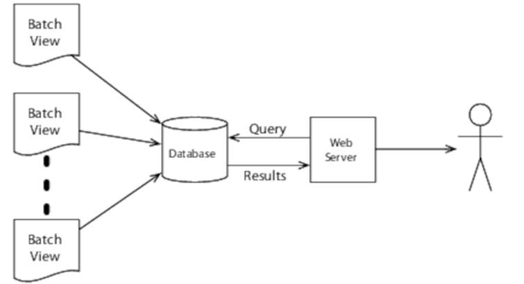
If we know ahead of time which queries we want to run against our raw data, we can precompute a batch view, which either directly contains the derived data that will be returned by those queries or contains data that can easily be combined to create it. Computing these batch views is the job of the Lambda Architecture’s batch layer.
As an example of the first type of batch view, consider building Wikipedia pages from a sequence of edits—the batch view will simply comprise the text of each page, built by combining all the edits of that page.
The second type of batch view is slightly more complex, so that’s what we’ll concentrate on for the remainder of today. We’re going to use Hadoop to build batch views that will allow us to query how many edits a Wikipedia contributor has made over a period of days.
Wikipedia Contributors
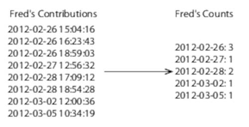
The kind of query that we’d ideally like to make is, “How many contributions did Fred Bloggs make between 3:15 p.m. on Tuesday, June 5, 2012, and 10:45 a.m. on Thursday, June 7, 2012?” To do so, however, we’d need to maintain and index a record of the exact time of every contribution. If we really need to make this kind of query, then we’ll need to pay the price, but in reality we’re unlikely to need to make queries at this fine a granularity—a day-by-day basis is likely to be more than enough.
So our batch view could consist of simple daily totals:
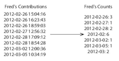
This would work well enough if we were always interested in periods of a few days, but queries for periods of several months would still require combining many values (potentially, for example, 365 to determine how many contributions a user had made in a year). We can decrease the amount of work required to answer this kind of query by keeping track of periods of both months and days:
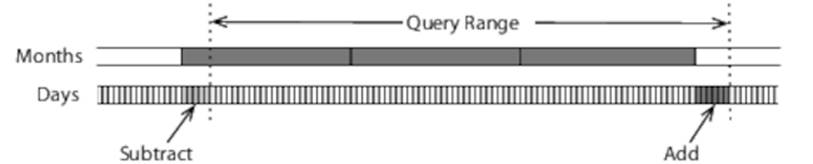
This would allow us to decrease the amount of work required to count a user’s contributions within a year from summing 365 values to 12. And we can handle periods that neither start nor finish at the beginning of a month by summing monthly values and either adding or subtracting daily values:
Contributor Logging
Sadly, we don’t have access to a live feed of Wikipedia contributors. But if we did, it might look something like this:
|
|
2012-09-01T14:18:13Z 123456789 1234 Fred Bloggs |
|
|
2012-09-01T14:18:15Z 123456790 54321 John Doe |
|
|
2012-09-01T14:18:16Z 123456791 6789 Paul Butcher |
|
|
⋮ |
The first column is a timestamp, the second is an identifier representing the contribution, the third is an identifier representing the user who made the contribution, and the remainder of the line is the username.
Although Wikipedia doesn’t publish such a feed, it does provide periodic XML dumps containing a full history (you’re looking for enwiki-latest-stub-meta-history).[69] The sample code for this chapter includes an ExtractWikiContributors project that will take one of these dumps and create a file of the preceding form.
In the next section we’ll construct a Hadoop job that takes these log files and generates the data required for our batch view.
Counting Contributions
As always, our Hadoop job consists of a mapper and a reducer. The mapper is very straightforward, simply parsing a line of the contributor log and generating a key/value pair in which the key is the contributor ID and the value is the timestamp of the contribution:
|
LambdaArchitecture/WikiContributorsBatch/src/main/java/com/paulbutcher/WikipediaContributors.java |
|
|
|
public static class Map extends Mapper<Object, Text, IntWritable, LongWritable> { |
|
|
|
|
|
public void map(Object key, Text value, Context context) |
|
|
throws IOException, InterruptedException { |
|
|
|
|
|
Contribution contribution = new Contribution(value.toString()); |
|
|
context.write(new IntWritable(contribution.contributorId), |
|
|
new LongWritable(contribution.timestamp)); |
|
|
} |
|
|
} |
Most of the work is done by the Contribution class:
|
LambdaArchitecture/WikiContributorsBatch/src/main/java/com/paulbutcher/Contribution.java |
|
|
Line 1 |
class Contribution { |
|
- |
static final Pattern pattern = Pattern.compile("^([^\\s]*) (\\d*) (\\d*) (.*)$"); |
|
- |
static final DateTimeFormatter isoFormat = ISODateTimeFormat.dateTimeNoMillis(); |
|
- |
|
|
5 |
public long timestamp; |
|
- |
public int id; |
|
- |
public int contributorId; |
|
- |
public String username; |
|
- |
|
|
10 |
public Contribution(String line) { |
|
- |
Matcher matcher = pattern.matcher(line); |
|
- |
if(matcher.find()) { |
|
- |
timestamp = isoFormat.parseDateTime(matcher.group(1)).getMillis(); |
|
- |
id = Integer.parseInt(matcher.group(2)); |
|
15 |
contributorId = Integer.parseInt(matcher.group(3)); |
|
- |
username = matcher.group(4); |
|
- |
} |
|
- |
} |
|
- |
} |
We could parse a log file line in various ways—in this case, we’re using a regular expression (line 2). If it matches, we use the ISODateTimeFormat class from the Joda-Time library to parse the timestamp and convert it to a long value representing the number of milliseconds since January 1, 1970 (line 13).[70] The contribution and contributor IDs are then just simple integers, and the contributor’s username is the remainder of the line.
Our reducer is more involved:
|
LambdaArchitecture/WikiContributorsBatch/src/main/java/com/paulbutcher/WikipediaContributors.java |
|
|
Line 1 |
public static class Reduce |
|
- |
extends Reducer<IntWritable, LongWritable, IntWritable, Text> { |
|
- |
static DateTimeFormatter dayFormat = ISODateTimeFormat.yearMonthDay(); |
|
- |
static DateTimeFormatter monthFormat = ISODateTimeFormat.yearMonth(); |
|
5 |
|
|
- |
public void reduce(IntWritable key, Iterable<LongWritable> values, |
|
- |
Context context) throws IOException, InterruptedException { |
|
- |
HashMap<DateTime, Integer> days = new HashMap<DateTime, Integer>(); |
|
- |
HashMap<DateTime, Integer> months = new HashMap<DateTime, Integer>(); |
|
10 |
for (LongWritable value: values) { |
|
- |
DateTime timestamp = new DateTime(value.get()); |
|
- |
DateTime day = timestamp.withTimeAtStartOfDay(); |
|
- |
DateTime month = day.withDayOfMonth(1); |
|
- |
incrementCount(days, day); |
|
15 |
incrementCount(months, month); |
|
- |
} |
|
- |
for (Entry<DateTime, Integer> entry: days.entrySet()) |
|
- |
context.write(key, formatEntry(entry, dayFormat)); |
|
- |
for (Entry<DateTime, Integer> entry: months.entrySet()) |
|
20 |
context.write(key, formatEntry(entry, monthFormat)); |
|
- |
} |
|
- |
} |
For each contributor, we build two HashMaps, days (line 8) and months (line 9). We populate these by iterating over timestamps (remember that values will be a list of timestamps) using the Joda-Time utility methods withTimeAtStartOfDay and withDayOfMonth to convert that timestamp to midnight on the day of the contribution and midnight on the first day of the month (lines 12 and 13, respectively). We then increment the relevant count in days and months using a simple utility method:
|
LambdaArchitecture/WikiContributorsBatch/src/main/java/com/paulbutcher/WikipediaContributors.java |
|
|
|
private void incrementCount(HashMap<DateTime, Integer> counts, DateTime key) { |
|
|
Integer currentCount = counts.get(key); |
|
|
if (currentCount == null) |
|
|
counts.put(key, 1); |
|
|
else |
|
|
counts.put(key, currentCount + 1); |
|
|
} |
Finally, once we’ve finished building our maps, we iterate over each map and generate an output for each day and month in which there was at least one contribution (lines 17 to 20).
This is slightly involved because, as we’ve seen, the output from a Hadoop job is always a set of key/value pairs, but what we want to output are three values—the contributor ID, a date (either a month or a day), and a count. We could do this by defining a composite value. This way, our key is the contributor ID and the value is a composite value containing the date and the count. But our case is simple enough that we can instead just use a string as the value type and format it appropriately with formatEntry:
|
LambdaArchitecture/WikiContributorsBatch/src/main/java/com/paulbutcher/WikipediaContributors.java |
|
|
|
private Text formatEntry(Entry<DateTime, Integer> entry, |
|
|
DateTimeFormatter formatter) { |
|
|
return new Text(formatter.print(entry.getKey()) + "\t" + entry.getValue()) |
|
|
} |
Here’s a section of this job’s output:
|
|
463 2001-11-24 1 |
|
|
463 2002-02-14 1 |
|
|
463 2001-11-26 6 |
|
|
463 2001-10-01 1 |
|
|
463 2002-02 1 |
|
|
463 2001-10 1 |
|
|
463 2001-11 7 |
This contains exactly the data that we need, but a collection of text files isn’t particularly convenient. In the next section we’ll talk about the serving layer, which indexes and combines the output of the batch layer.
![]()
Joe asks:
Can We Generate Batch Views Incrementally?
The batch layer we’ve described so far recomputes entire batch views from scratch each time it’s run. This will certainly work, but it’s probably performing more work than necessary—why not update batch views incrementally with the new data that’s arrived since the last time the batch view was generated?
The simple answer is that there’s nothing to stop you from doing so, and this can be a useful optimization. But you can’t rely exclusively on incremental updates—much of the power of the Lambda Architecture derives from the fact that we can always rebuild from scratch if we need to. So feel free to implement an incremental algorithm if the optimization is worth the additional effort, but recognize that this can never be a replacement for recomputation.
Completing the Picture
The batch layer isn’t enough on its own to create a complete end-to-end application. That requires the next element of the Lambda Architecture—the serving layer.
The Serving Layer
The batch view we’ve just generated needs to be indexed so that we can make queries against it, and we need somewhere to put the application logic that decides how to combine elements of the batch view to satisfy a particular query. This is the duty of the serving layer:
We’re going to leave the serving layer as an exercise for the reader, as it has little relevance to the subject matter of this book, but it’s worth mentioning one particular aspect of it—the database.
Although you could build the serving layer on top of a traditional database, its access patterns are rather different from a traditional application. In particular, there’s no requirement for random writes—the only time the database is updated is when the batch views are updated, which requires a batch update.
Therefore a category emerges of serving-layer databases optimized for this usage pattern, the most well-known of which are ElephantDB and Voldemort.[71][72]
Almost Nirvana
Taken together, the batch and serving layers give us a data system that addresses all the problems we identified at the beginning of the day:
The batch layer runs in an infinite loop, regenerating batch views from our raw data. Each time a batch run completes, the serving layer updates its database.
Because it only ever operates on immutable raw data, the batch layer can easily exploit parallelism. Raw data can be distributed across a cluster of machines, enabling batch views to be recomputed in an acceptable period of time even when dealing with terabytes of input.
The immutability of raw data also means that the system is intrinsically hardened against both technical failure and human error. Not only is it much easier to back up raw data, but if there’s a bug, the worst that can happen is that batch views are temporarily incorrect—we can always correct them by fixing the bug and recomputing them.
Finally, because we retain all raw data, we can always generate any report or analysis that might occur to us in the future.
There’s an obvious problem, though—latency. If the batch layer takes an hour to run, then our batch views will always be at least an hour out-of-date. This is where tomorrow’s subject, the speed layer, comes into play.
Day 2 Wrap-Up
This brings us to the end of day 2. In day 3 we’ll complete our picture of the Lambda Architecture by looking at the speed layer.
What We Learned in Day 2
Information can be divided into raw data and derived information. Raw data is eternally true and therefore immutable. The batch layer of the Lambda Architecture leverages this to allow us to create systems that are
· highly parallel, enabling terabytes of data to be processed;
· simple, making them both easier to create and less error prone;
· tolerant of both technical failure and human error; and
· capable of supporting both day-to-day operations and historical reporting and analysis.
The primary drawback of the batch layer is latency, which the Lambda Architecture addresses by running the speed layer alongside.
Day 2 Self-Study
Find
· The approaches we’ve discussed here are not the only way to tackle building a data system that leverages Hadoop—other options include HBase, Pig, and Hive. All three of these have more in common with a traditional data system than what we’ve seen today. Pick one and compare it to the Lambda Architecture’s batch layer. When might you choose one, and when the other?
Do
· Finish the system we built today by creating a serving layer that takes the output of the batch layer, puts it in a database, and allows queries about the number of edits made by a particular user over a range of days. You can build it either on top of a traditional database or on top of ElephantDB.
· Extend the preceding to build batch views incrementally—to do this, you will need to provide the Hadoop cluster with access to the serving layer’s database. How much more efficient is it? Is it worth the additional effort? For which types of application would incremental batch view construction make sense? For which would it not?
Day 3: The Speed Layer
As we saw yesterday, the batch layer of the Lambda Architecture solves all the problems we identified with traditional data systems, but it does so at the expense of latency. The speed layer exists to solve that problem. The following figure shows how the batch and speed layers work together:
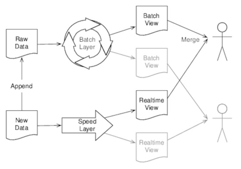
Figure 22. The Lambda Architecture
As new data arrives, we both append it to the raw data that the batch layer works on and send it to the speed layer. The speed layer generates real-time views, which are combined with batch views to create fully up-to-date answers to queries.
Real-time views contain only information derived from the data that arrived since the batch views were last generated and are discarded when the data they were built from is processed by the batch layer.
Today we’ll see how to use Storm to create the speed layer.[73]
Designing the Speed Layer
Different applications have different interpretations of real time—some require new data to be available in seconds, some in milliseconds. But whatever your particular application’s performance requirements are, it’s unlikely that they can be met with a pure batch-oriented approach.
Building the speed layer is therefore intrinsically more difficult than building the batch layer because it’s forced to take an incremental approach. This in turn means that it can’t restrict itself to only processing raw data and can’t rely on the nice properties of raw data we identified yesterday. So we’re back to traditional databases that support random writes and all the complexity (locking, transactions, and so forth) that comes with them.
On the plus side, the speed layer only needs to handle that portion of our data that hasn’t already been handled by the batch layer (typically a few hours’ worth). Once the batch layer catches up, older data can be expired from the speed layer.
Synchronous or Asynchronous?
One obvious way to build the speed layer would be to do so as a traditional synchronous database application. Indeed, you can think of a traditional database application as a degenerate case of the Lambda Architecture in which the batch layer never runs:
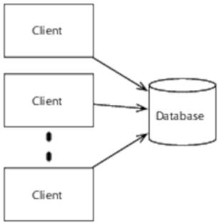
In this approach, clients communicate directly with the database and block while it’s processing each update. This is a perfectly reasonable approach, and for some applications it may be the only one that meets their operational requirements. But in many cases, an asynchronous architecture will be better:
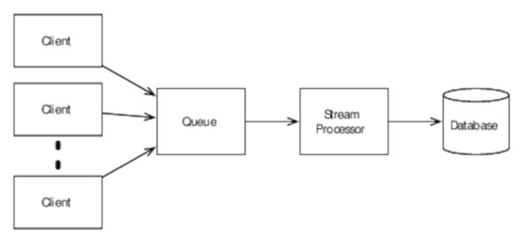
In this approach, clients add updates to a queue (implemented with, for example, Kafka or Kestrel[74][75]) as they arrive and without blocking. A stream processor then handles these updates in turn and performs the database update.
Using a queue decouples clients from database updates, making it more complex to coordinate updates with other actions. For applications in which this is acceptable, the benefits are significant:
· Because clients don’t block, fewer clients can handle higher volumes of data, leading to greater throughput.
· Spikes in demand might lead to a synchronous system timing out or dropping updates as clients or the database becoming overloaded. An asynchronous system, by contrast, will simply fall behind, storing unhandled updates in the queue and catching up when demand returns to normal levels.
· As we’ll see during the remainder of today, the stream processor can exploit parallelism, distributing processing over multiple computing resources in order to provide both fault tolerance and improved performance.
For these reasons, and because synchronous speed-layer implementations are largely uninteresting as far as parallelism and concurrency are concerned, we’re not going to consider them further in this book. Before we look at an asynchronous implementation, however, we should touch on one other subject—expiring data.
Expiring Data
If your batch layer takes (say) two hours to run, you would be forgiven for thinking that your speed layer will need to handle two hours’ worth of data. In fact, it will need to handle up to twice that amount, as shown in the figure:
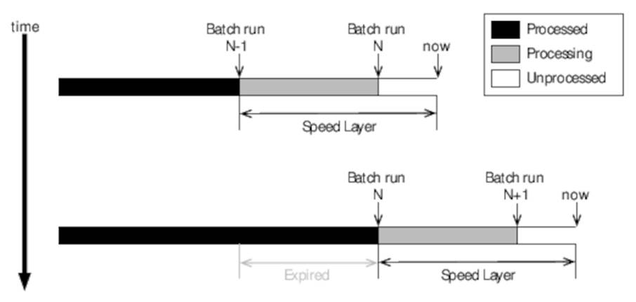
Figure 23. Expiring data in the speed layer
Imagine that batch run N-1 has just completed and batch run N is just about to start. If each takes two hours to run, that means that our batch views will be two hours out-of-date. The speed layer therefore needs to serve requests for those two hours’ worth of data plus any data that arrives before batch run N completes, for a total of four hours’ worth.
When batch run N does complete, we then need to expire the data that represents the oldest two hours but still retain the most recent two hours’ worth. It is certainly possible to come up with schemes that allow you to do this, but the easiest solution can be to run two copies of the speed layer in parallel and ping-pong between them, as shown in Figure 24, Ping-pong speed layers.
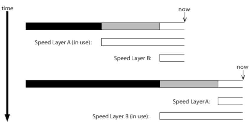
Figure 24. Ping-pong speed layers
Whenever a batch run completes and new data becomes available in the batch views, we switch from the speed layer that’s currently serving queries to its counterpart with more recent data. The now-idle speed layer then clears its database and starts building a new set of views from scratch, starting at the point where the new batch run started.
Not only does this approach save us from having to identify which data to delete from the speed layer’s database, but it also improves performance and reliability by ensuring that each iteration of the speed layer starts from a clean database. The cost, of course, is that we have to maintain two copies of the speed layer’s data and twice the computing resources, but this cost is unlikely to be significant in relative terms, given that the speed layer is only handling a very small fraction of the total data.
Storm
We’re going to spend the rest of today looking at the outline of an asynchronous speed layer implementation in Storm. Storm is a big subject, so we’ll cover it in only enough detail to give a taste—refer to the Storm documentation for more depth.[76]
Storm aims to do for real-time processing what Hadoop has for batch processing—to make it easy to distribute computation across multiple machines in order to improve both performance and fault tolerance.
Spouts, Bolts, and Topologies
A Storm system processes streams of tuples. Storm’s tuples are similar to those we saw in Chapter 5, Actors, the primary difference being that unlike Elixir’s tuples, the elements of a Storm tuple are named.
Tuples are created by spouts and processed by bolts, which can create tuples in turn. Spouts and bolts are connected by streams to form a topology. Here’s a simple topology in which a single spout creates tuples that are processed by a pipeline of bolts:
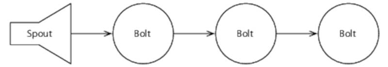
Figure 25. A simple topology
Topologies can be much more complex than this—bolts can consume multiple streams, and a single stream can be consumed by multiple bolts to create a directed acyclic graph, or DAG:
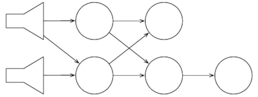
Figure 26. A complex topology
Even our simple pipeline topology is more complex than it appears, however, because spouts and bolts are both parallel and distributed.
Workers
Not only do spouts and bolts run in parallel with each other, but they are also internally parallel—each is implemented as a set of workers. Figure 27, Spout and bolt workers shows what our simple pipeline topology might look like if each spout and bolt had three workers.
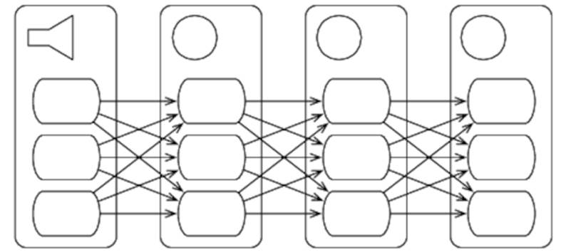
Figure 27. Spout and bolt workers
As our diagram shows, the workers of each node of the pipeline can send tuples to any of the workers in their downstream node. We’ll see how to control exactly which worker receives a tuple when we discuss stream grouping later.
Finally, workers are distributed—if we’re running on a four-node cluster, for example, then our spout’s workers might be on nodes 1, 2, and 3; the first bolt’s workers might be on nodes 2 and 4 (two on node 2, one on node 4); and so on.
The beauty of Storm is that we don’t need to explicitly worry about this distribution—all we need to do is specify our topology, and the Storm runtime allocates workers to nodes and makes sure that tuples are routed appropriately.
Fault Tolerance
A large part of the reason for distributing a single spout or bolt’s workers across multiple machines is fault tolerance. If one of the machines in our cluster fails, our topology can continue to operate by routing tuples to the machines that are still operating.
Storm keeps track of the dependencies between tuples—if a particular tuple’s processing isn’t completed, Storm fails and retries the spout tuple(s) upon which it depends. This means that, by default, Storm provides an “at least once” processing guarantee. Applications need to be aware of the fact that tuples might be retried and continue to function correctly if they are.
Enough theory—let’s see how we can use Storm to create an outline implementation of a speed layer for our Wikipedia contributor application.
![]()
Joe asks:
What If My Application Can’t Handle Retries?
Storm’s default “at least once” semantics are adequate for most applications, but some need a stronger “exactly once” processing guarantee.
Storm supports “exactly once” semantics via the Trident API.[77] Trident is not covered in this book.
Counting Contributions with Storm
Here’s a possible topology for our speed layer:
We start with a spout that imports contributor logs and converts them to a stream of tuples. This is consumed by a bolt that parses log entries and outputs a stream of parsed log entries. Finally, this stream is in turn consumed by a bolt that updates a database containing our real-time view.
We’re going to build a slightly different topology from this, however, for a couple of reasons. First, we don’t have access to a log of Wikipedia contributors; second, the details of updating a database are uninteresting from our point of view (with our focus on parallelism and concurrency). The following figure shows what we’re going to build instead.
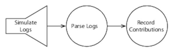
We’re going to create a spout that simulates a Wikipedia contributor feed and then a parser, and finally we’ll record the real-time views in memory. This wouldn’t be a good production approach, but it will serve our purpose of exploring Storm.
Simulating the Contribution Log
Here’s the code for our spout, which simulates a contributor feed by generating random log entries:
|
LambdaArchitecture/WikiContributorsSpeed/src/main/java/com/paulbutcher/RandomContributorSpout.java |
|
|
Line 1 |
public class RandomContributorSpout extends BaseRichSpout { |
|
- |
|
|
- |
private static final Random rand = new Random(); |
|
- |
private static final DateTimeFormatter isoFormat = |
|
5 |
ISODateTimeFormat.dateTimeNoMillis(); |
|
- |
|
|
- |
private SpoutOutputCollector collector; |
|
- |
private int contributionId = 10000; |
|
- |
|
|
10 |
public void open(Map conf, TopologyContext context, |
|
- |
SpoutOutputCollector collector) { |
|
- |
|
|
- |
this.collector = collector; |
|
- |
} |
|
15 |
|
|
- |
public void declareOutputFields(OutputFieldsDeclarer declarer) { |
|
- |
declarer.declare(new Fields("line")); |
|
- |
} |
|
- |
|
|
20 |
public void nextTuple() { |
|
- |
Utils.sleep(rand.nextInt(100)); |
|
- |
++contributionId; |
|
- |
String line = isoFormat.print(DateTime.now()) + " " + contributionId + " " + |
|
- |
rand.nextInt(10000) + " " + "dummyusername"; |
|
25 |
collector.emit(new Values(line)); |
|
- |
} |
|
- |
} |
We indicate that we’re creating a spout by deriving from BaseRichSpout (line 1). Storm calls our open method (line 10) during initialization—we simply keep a record of the SpoutOutputCollector, which is where we’ll send our output. Storm also calls our declareOutputFields method (line 16) during initialization to find out how the tuples generated by this spout are structured—in this case, the tuples have a single field called line.
The method that does most of the work is nextTuple (line 20). We start by sleeping for a random interval of up to 100 ms, and then we create a string of the same format we saw in Contributor Logging, which we output by calling collector.emit.
These lines will be passed to the parser bolt, which we’ll see next.
Parsing Log Entries
Our parser bolt takes tuples containing log lines, parses them, and outputs tuples with four fields, one for each component of the log line:
|
LambdaArchitecture/WikiContributorsSpeed/src/main/java/com/paulbutcher/ContributionParser.java |
|
|
Line 1 |
class ContributionParser extends BaseBasicBolt { |
|
2 |
public void declareOutputFields(OutputFieldsDeclarer declarer) { |
|
3 |
declarer.declare(new Fields("timestamp", "id", "contributorId", "username")); |
|
4 |
} |
|
5 |
public void execute(Tuple tuple, BasicOutputCollector collector) { |
|
6 |
Contribution contribution = new Contribution(tuple.getString(0)); |
|
7 |
collector.emit(new Values(contribution.timestamp, contribution.id, |
|
8 |
contribution.contributorId, contribution.username)); |
|
9 |
} |
|
10 |
} |
We indicate that we’re creating a bolt by deriving from BaseBasicBolt (line 1). As with our spout, we implement declareOutputFields (line 2) to let Storm know how our output tuples are structured—in this case they have four fields, called timestamp, id, contributorId, and username.
The method that does most of the work is execute (line 5). In this case, it uses the same Contributor as the batch layer to parse the log line into its components and then calls contributor.emit to output the tuple.
These parsed tuples will be passed to a bolt that keeps a record of each contributor’s contributions, which we’ll see next.
Recording Contributions
Our final bolt maintains a simple in-memory database (a map from contributor IDs to a set of contribution timestamps) of each contributor’s contributions:
|
LambdaArchitecture/WikiContributorsSpeed/src/main/java/com/paulbutcher/ContributionRecord.java |
|
|
Line 1 |
class ContributionRecord extends BaseBasicBolt { |
|
- |
private static final HashMap<Integer, HashSet<Long>> timestamps = |
|
- |
new HashMap<Integer, HashSet<Long>>(); |
|
- |
|
|
5 |
public void declareOutputFields(OutputFieldsDeclarer declarer) { |
|
- |
} |
|
- |
public void execute(Tuple tuple, BasicOutputCollector collector) { |
|
- |
addTimestamp(tuple.getInteger(2), tuple.getLong(0)); |
|
- |
} |
|
10 |
|
|
- |
private void addTimestamp(int contributorId, long timestamp) { |
|
- |
HashSet<Long> contributorTimestamps = timestamps.get(contributorId); |
|
- |
if (contributorTimestamps == null) { |
|
- |
contributorTimestamps = new HashSet<Long>(); |
|
15 |
timestamps.put(contributorId, contributorTimestamps); |
|
- |
} |
|
- |
contributorTimestamps.add(timestamp); |
|
- |
} |
|
- |
} |
In this case we’re not generating any output, so declareOutputFields is empty (line 5). Our execute method (line 7) simply extracts the relevant fields from its input tuple and passes them to addTimestamp, which simply adds the timestamp to the set associated with the contributor.
Finally, let’s see how to build a topology that uses our spout and bolts.
![]()
Joe asks:
Why Record a Set of Timestamps?
The batch views we saw in Day 2: The Batch Layer, just recorded per-day and per-month counts for each contributor. So why do our real-time views record full timestamps?
Firstly, as we discussed earlier, our real-time views only need to record a few hours’ worth of data, so the cost of storing and querying a full set of timestamps is relatively low. But there’s a more important reason—adding an item to a set is idempotent.
Recall that Storm supports “at least once” semantics (see Fault Tolerance), so tuples might be retried. An idempotent operation gives the same result no matter how many times it’s performed, which is exactly what we need to be able to cope with tuples being retried.
Building the Topology
Something might be worrying you about ContributionRecord—given that bolts have multiple workers, how do we ensure that we maintain only a single set of timestamps for each contributor? We’ll see how when we construct our topology.
|
LambdaArchitecture/WikiContributorsSpeed/src/main/java/com/paulbutcher/WikiContributorsTopology.java |
|
|
Line 1 |
public class WikiContributorsTopology { |
|
- |
|
|
- |
public static void main(String[] args) throws Exception { |
|
- |
|
|
5 |
TopologyBuilder builder = new TopologyBuilder(); |
|
- |
|
|
- |
builder.setSpout("contribution_spout", new RandomContributorSpout(), 4); |
|
- |
|
|
- |
builder.setBolt("contribution_parser", new ContributionParser(), 4). |
|
10 |
shuffleGrouping("contribution_spout"); |
|
- |
|
|
- |
builder.setBolt("contribution_recorder", new ContributionRecord(), 4). |
|
- |
fieldsGrouping("contribution_parser", new Fields("contributorId")); |
|
- |
|
|
15 |
LocalCluster cluster = new LocalCluster(); |
|
- |
Config conf = new Config(); |
|
- |
cluster.submitTopology("wiki-contributors", conf, builder.createTopology()); |
|
- |
|
|
- |
Thread.sleep(10000); |
|
20 |
|
|
- |
cluster.shutdown(); |
|
- |
} |
|
- |
} |
We start by creating a TopologyBuilder (line 5) and we add an instance of our spout with setSpout (line 7), the second argument to which is a parallelism hint. As its name suggests, this is a hint, not an instruction, but for our purposes, we can think of it as instructing Storm to create four workers for our spout. For a full description of how to control parallelism in Storm, see “What Makes a Running Topology: Worker Processes, Executors and Tasks.”[78]
Next, we add an instance of our ContributionParser bolt with setBolt (line 9). We tell Storm that this bolt should take its input from our spout by calling shuffleGrouping, passing it the name we gave to the spout, which brings us to the subject of stream grouping.
Stream Grouping
Storm’s stream grouping answers the question about which workers receive which tuples. The shuffle grouping we’re using for our parser bolt is the simplest—it simply sends tuples to a random worker.
Our contribution recorder bolt uses a fields grouping (line 12), which guarantees that all tuples with the same values for a set of fields (in our case, the contributorId field) are always sent to the same worker. This is how we guarantee that we maintain only a single set of timestamps for each contributor, answering the question we posed at the start of this section.
A Local Cluster
Setting up a Storm cluster isn’t a huge job, but it’s beyond the scope of this book. And sadly, as it’s a relatively young technology, nobody’s currently providing managed Storm clusters that we can leverage. So we’ll run our topology locally by creating a LocalCluster (line 17).
Our sample then allows this topology to run for ten seconds and then shuts it down with cluster.shutdown. In production, of course, we would need to provide a means to shut our topology down when the real-time views it’s handling are no longer necessary because the batch layer has caught up.
Day 3 Wrap-Up
That brings us to the end of day 3 and the end of our discussion of the Lambda Architecture’s speed layer.
What We Learned in Day 3
The speed layer completes the Lambda Architecture by providing real-time views of data that’s arrived since the most recent batch views were built. The speed layer can be synchronous or asynchronous—Storm is one means by which we can build an asynchronous speed layer:
· Storm processes streams of tuples in real time. Tuples are created by spouts and processed by bolts, arranged in a topology.
· Spouts and bolts each have multiple workers that run in parallel and are distributed across the nodes of a cluster.
· By default, Storm provides “at least once” semantics—bolts need to handle tuples being retried.
Day 3 Self-Study
Find
· Trident is a high-level API built on top of Storm that, among other things, provides “exactly once” semantics as well as Storm’s “at least once” default semantics. When does it make sense to use Trident and when the low-level Storm API?
· Which other stream groupings does Storm support in addition to shuffle and fields groupings?
Do
· Create a Storm cluster and submit today’s example so that it runs distributed instead of locally.
· Create a bolt that keeps track of the total number of contributions that have been made each minute and a topology in which both it and ContributionRecord consume the output of ContributionParser.
· Today’s example made use of BaseBasicBolt, which automatically acknowledges tuples. Modify it to use BaseRichBolt—you will need to acknowledge tuples explicitly. How could you create a bolt that processes multiple tuples before acknowledging them?
Wrap-Up
The Lambda Architecture brings together many concepts we’ve covered elsewhere:
· The insight that raw data is eternally true should remind you of Clojure’s separation of identity and state.
· Hadoop’s approach of parallelizing a problem by splitting it into a map over a data structure followed by a reduce should remind you of much of what we saw when we looked at parallel functional programming.
· Like actors, the Lambda Architecture distributes processing over a cluster to both improve performance and provide fault tolerance in the face of hardware failure.
· Storm’s streams of tuples have much in common with the message passing we saw in both actors and CSP.
Strengths
The Lambda Architecture is all about handling huge quantities of data—problems where traditional data-processing architectures are struggling to cope. It’s particularly well suited to reporting and analytics—the kinds of problems that might have been addressed with a data warehouse in the past.
Weaknesses
The Lambda Architecture’s great strength—its focus on huge quantities of data—is also its weakness. Unless your data is measured in tens of gigabytes or more, its overhead (both computational and intellectual) is unlikely to be worth the benefit.
Alternatives
The Lambda Architecture isn’t tied to MapReduce—the batch layer could be implemented with any distributed batch-processing system.
With that in mind, Apache Spark is particularly interesting.[79] Spark is a cluster computing framework that implements a DAG execution engine, allowing a number of algorithms (most notably graph algorithms) to be expressed more naturally than they can be with MapReduce. It also has an associated streaming API, meaning that both the batch and speed layers could be implemented within Spark.[80]
Final Thoughts
The Lambda Architecture is a fitting end to this book, leveraging as it does many of the techniques we’ve seen in earlier chapters. It’s a powerful demonstration of how parallelism and concurrency allow us to tackle problems that would otherwise be intractable.
In the last chapter, we’ll review what we’ve seen over the last seven weeks and examine the broad themes that have emerged.
Footnotes
|
[55] |
http://www.manning-sandbox.com/message.jspa?messageID=126599 |
|
[56] |
http://research.google.com/archive/mapreduce.html |
|
[57] |
http://hadoop.apache.org |
|
[58] |
http://aws.amazon.com/elasticmapreduce/ |
|
[59] |
http://aws.amazon.com/cli/ |
|
[60] |
http://docs.aws.amazon.com/ElasticMapReduce/latest/DeveloperGuide/emr-cli-reference.html |
|
[61] |
http://hortonworks.com |
|
[62] |
http://www.cloudera.com |
|
[63] |
http://www.mapr.com |
|
[64] |
http://docs.aws.amazon.com/ElasticMapReduce/latest/DeveloperGuide/emr-plan-hadoop-version.html |
|
[65] |
http://aws.amazon.com/s3/ |
|
[66] |
http://aws.amazon.com/ec2/instance-types/ |
|
[67] |
http://mahout.apache.org |
|
[68] |
https://github.com/apache/mahout/blob/trunk/integration/src/main/java/org/apache/mahout/text/wikipedia/XmlInputFormat.java |
|
[69] |
http://dumps.wikimedia.org/enwiki |
|
[70] |
http://www.joda.org/joda-time/ |
|
[71] |
https://github.com/nathanmarz/elephantdb |
|
[72] |
http://www.project-voldemort.com/voldemort/ |
|
[73] |
http://storm.incubator.apache.org |
|
[74] |
http://kafka.apache.org |
|
[75] |
http://robey.github.io/kestrel/ |
|
[76] |
http://storm.incubator.apache.org/documentation/Home.html |
|
[77] |
http://storm.incubator.apache.org/documentation/Trident-tutorial.html |
|
[78] |
http://storm.incubator.apache.org/documentation/Understanding-the-parallelism-of-a-Storm-topology.html |
|
[79] |
http://spark.apache.org |
|
[80] |
http://spark.apache.org/streaming/ |
All materials on the site are licensed Creative Commons Attribution-Sharealike 3.0 Unported CC BY-SA 3.0 & GNU Free Documentation License (GFDL)
If you are the copyright holder of any material contained on our site and intend to remove it, please contact our site administrator for approval.
© 2016-2026 All site design rights belong to S.Y.A.