Seven Concurrency Models in Seven Weeks (2014)
Chapter 7. Data Parallelism
Data parallelism is like an eight-lane highway. Even though each vehicle is traveling at a relatively modest speed, the number of cars that pass a particular point is huge because many vehicles can travel side-by-side.
All the approaches we’ve discussed so far have been applicable to a wide variety of programming problems. Data-parallel programming, by contrast, is relevant only to a much narrower range. As its name suggests, it’s a parallel-programming technique, not a concurrency technique (recall that concurrency and parallelism are related but different—see Concurrent or Parallel?).
The Supercomputer Hidden in Your Laptop
In this chapter we’re going to see how to leverage the supercomputer hidden in your laptop—the graphics processing unit or GPU. A modern GPU is a powerful data-parallel processor, capable of eclipsing the CPU when used for number-crunching, a practice that is commonly referred to asgeneral-purpose computing on the GPU or GPGPU programming.
Over the years, a number of technologies have emerged to abstract away from the details of GPU implementation. We’ll be using the Open Computing Language, or OpenCL, to write GPGPU code.[48]
In day 1 we’ll see the basics of constructing an OpenCL kernel, together with the host program that compiles and executes it. In day 2 we’ll look at how a kernel is mapped onto hardware in more depth. Finally, in day 3 we’ll see how OpenCL can interoperate with graphics code written with the Open Graphics Library, or OpenGL.[49]
Day 1: GPGPU Programming
Today we’ll see how to create a simple GPGPU program that multiplies two arrays in parallel, and then we’ll benchmark it to see just how much faster the GPU is than the CPU. First, though, we’ll spend a little time examining what makes a GPU so powerful when it comes to number-crunching.
Graphics Processing and Data Parallelism
Computer graphics is all about manipulating data—huge amounts of data. And doing it quickly. A scene in a 3D game is constructed from a myriad of tiny triangles, each of which needs to have its position on the screen calculated in perspective relative to the viewpoint, clipped, lit, and textured twenty-five or more times a second.
The great thing about this is that although the amount of data that needs to be processed is huge, the actual operations on that data are relatively simple vector or matrix operations. This makes them very amenable to data parallelization, in which multiple computing units perform the same operations on different items of data in parallel.
Modern GPUS are exceptionally sophisticated, powerful parallel processors capable of rendering billions of triangles a second. The good news is that although they were originally designed with graphics alone in mind, their capabilities have evolved to the point that they’re useful for a much wider range of applications.
Data parallelism can be implemented in many different ways. We’ll look briefly at a couple of them: pipelining and multiple ALUs.
Pipelining
Although we tend to think of multiplying two numbers as a single atomic operation, down at the level of the gates on a chip, it actually takes several steps. These steps are typically arranged as a pipeline:
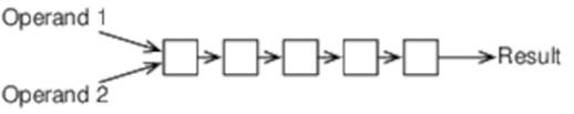
For the five-element pipeline shown here, if it takes a single clock cycle for each step to complete, multiplying a pair of numbers will take five clock cycles. But if we have lots of numbers to multiply, things get much better because (assuming our memory subsystem can supply the data fast enough) we can keep the pipeline full:
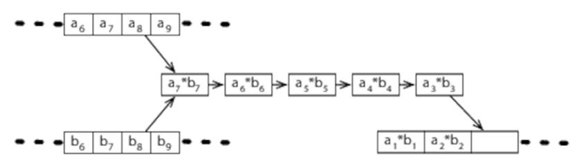
So multiplying a thousand pairs of numbers takes a whisker over a thousand clock cycles, not the five thousand we might expect from the fact that multiplying a single pair takes five clock cycles.
Multiple ALUs
The component within a CPU that performs operations such as multiplication is commonly known as the arithmetic logic unit, or ALU:

Couple multiple ALUs with a wide memory bus that allows multiple operands to be fetched simultaneously, and operations on large amounts of data can again be parallelized, as shown in Figure 12, Large Amounts of Data Parallelized with Multiple ALUs.
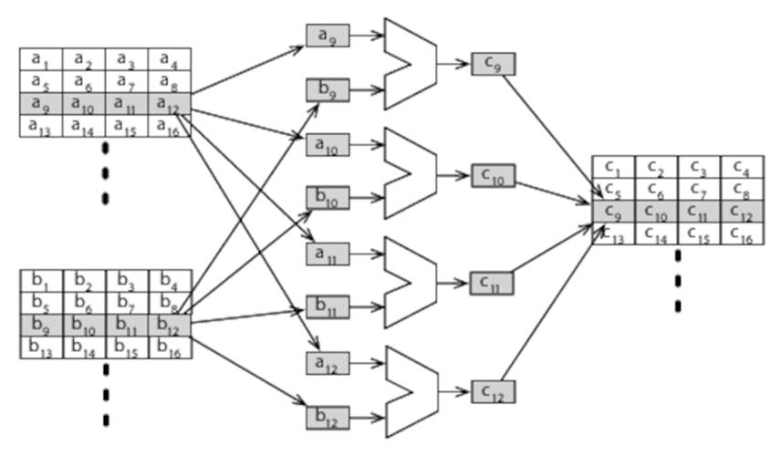
Figure 12. Large Amounts of Data Parallelized with Multiple ALUs
GPUs typically have a 256-bit or wider memory bus, allowing (for example) eight or more 32-bit floating-point numbers to be fetched at a time.
A Confused Picture
To achieve their performance, real-world GPUs combine pipelining and multiple ALUs with a wide range of other techniques that we’ll not cover here. By itself, this would make understanding the details of a single GPU complex. Unfortunately, there’s little commonality between differentGPUs (even those produced by a single manufacturer). If we had to write code that directly targeted a particular architecture, GPGPU programming would be a nonstarter.
OpenCL targets multiple architectures by defining a C-like language that allows us to express a parallel algorithm abstractly. Each different GPU manufacturer then provides its own compilers and drivers that allow that program to be compiled and run on its hardware.
Our First OpenCL Program
To parallelize our array multiplication task with OpenCL, we need to divide it up into work-items that will then be executed in parallel.
Work-Items
If you’re used to writing parallel code, you will be used to worrying about the granularity of each parallel task. Typically, if each task performs too little work, your code performs badly because thread creation and communication overheads dominate.
OpenCL work-items, by contrast, are typically very small. To multiply two 1,024-element arrays pairwise, for example, we could create 1,024 work-items (see Figure 13, Work Items for Pairwise Multiplication).
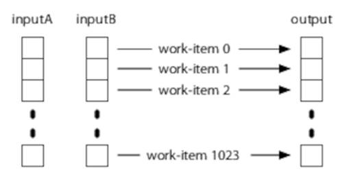
Figure 13. Work Items for Pairwise Multiplication
Your task as a programmer is to divide your problem into the smallest work-items you can. The OpenCL compiler and runtime then worry about how best to schedule those work-items on the available hardware so that that hardware is utilized as efficiently as possible.
Optimizing OpenCL
You won’t be surprised to hear that the real-world picture isn’t quite this simple. Optimizing an OpenCL application often involves thinking carefully about the available resources and providing hints to the compiler and runtime to help them schedule your work-items. Sometimes this includes restricting the available parallelism for efficiency purposes.
As always, however, premature optimization is the root of all programming evil. In the majority of cases, you should aim for maximum parallelism and the smallest possible work-items and worry about optimization only afterward.
Kernels
We specify how each work-item should be processed by writing an OpenCL kernel. Here’s a kernel that we could use to implement the preceding:
|
DataParallelism/MultiplyArrays/multiply_arrays.cl |
|
|
|
__kernel void multiply_arrays(__global const float* inputA, |
|
|
__global const float* inputB, |
|
|
__global float* output) { |
|
|
|
|
|
int i = get_global_id(0); |
|
|
output[i] = inputA[i] * inputB[i]; |
|
|
} |
This kernel takes pointers to two input arrays, inputA and inputB, and an output array, output. It calls get_global_id to determine which work-item it’s handling and then simply writes the result of multiplying the corresponding elements of inputA and inputB to the appropriate element ofoutput.
To create a complete program, we need to embed our kernel in a host program that performs the following steps:
1. Create a context within which the kernel will run together with a command queue.
2. Compile the kernel.
3. Create buffers for input and output data.
4. Enqueue a command that executes the kernel once for each work-item.
5. Retrieve the results.
The OpenCL standard defines both C and C++ bindings. However, unofficial bindings are available for most major languages, so you can write your host program in almost any language you like. We’re going to stick to C to start with because that’s the language the OpenCL standard uses and because it gives the best picture of what’s going on under the hood. In day 3 we’ll see a host program written in Java.
In the next few sections, we’ll put together a complete OpenCL host program. To make the underlying structure as clear as possible, I’m going to play a bit fast and loose and not include any error handling—don’t worry, we’ll come back to this later. You’ll also notice that there are a lot ofNULL arguments to functions—again, don’t worry about these too much right now; we’ll revisit the API in more detail after we’ve got a better feeling for the big picture.
Create a Context
An OpenCL context represents an environment within which OpenCL kernels can execute. To create a context, we first need to identify the platform that we want to use and which devices within that platform we want to execute our kernel (we’ll talk about platforms and devices in more detail later):
|
DataParallelism/MultiplyArrays/multiply_arrays.c |
|
|
|
cl_platform_id platform; |
|
|
clGetPlatformIDs(1, &platform, NULL); |
|
|
|
|
|
cl_device_id device; |
|
|
clGetDeviceIDs(platform, CL_DEVICE_TYPE_GPU, 1, &device, NULL); |
|
|
|
|
|
cl_context context = clCreateContext(NULL, 1, &device, NULL, NULL, NULL); |
We want a simple context that only contains a single GPU, so after identifying a platform with clGetPlatformIDs, we pass CL_DEVICE_TYPE_GPU to clGetDeviceIDs to get the ID of a GPU. Finally, we create a context by passing that device ID to clCreateContext.
Create a Command Queue
Now that we have a context, we can use it to create a command queue:
|
DataParallelism/MultiplyArrays/multiply_arrays.c |
|
|
|
cl_command_queue queue = clCreateCommandQueue(context, device, 0, NULL); |
The clCreateCommandQueue method takes a context and a device and returns a queue that enables commands to be sent to that device.
Compile the Kernel
Next we need to compile our kernel into code that will run on the device:
|
DataParallelism/MultiplyArrays/multiply_arrays.c |
|
|
|
char* source = read_source("multiply_arrays.cl"); |
|
|
cl_program program = clCreateProgramWithSource(context, 1, |
|
|
(const char**)&source, NULL, NULL); |
|
|
free(source); |
|
|
clBuildProgram(program, 0, NULL, NULL, NULL, NULL); |
|
|
cl_kernel kernel = clCreateKernel(program, "multiply_arrays", NULL); |
We start by reading the source code for the kernel from multiply_arrays.cl into a string (you can see the source of read_source in the code that accompanies the book) that is then passed to clCreateProgramWithSource. That’s then built with clBuildProgram and turned into a kernel withclCreateKernel.
Create Buffers
Kernels work on data stored within buffers:
|
DataParallelism/MultiplyArrays/multiply_arrays.c |
|
|
|
#define NUM_ELEMENTS 1024 |
|
|
cl_float a[NUM_ELEMENTS], b[NUM_ELEMENTS]; |
|
|
random_fill(a, NUM_ELEMENTS); |
|
|
random_fill(b, NUM_ELEMENTS); |
|
|
cl_mem inputA = clCreateBuffer(context, CL_MEM_READ_ONLY | CL_MEM_COPY_HOST_PTR, |
|
|
sizeof(cl_float) * NUM_ELEMENTS, a, NULL); |
|
|
cl_mem inputB = clCreateBuffer(context, CL_MEM_READ_ONLY | CL_MEM_COPY_HOST_PTR, |
|
|
sizeof(cl_float) * NUM_ELEMENTS, b, NULL); |
|
|
cl_mem output = clCreateBuffer(context, CL_MEM_WRITE_ONLY, |
|
|
sizeof(cl_float) * NUM_ELEMENTS, NULL, NULL); |
We start by creating two arrays, a and b, both of which we fill with random values with random_fill:
|
DataParallelism/MultiplyArrays/multiply_arrays.c |
|
|
|
void random_fill(cl_float array[], size_t size) { |
|
|
for (int i = 0; i < size; ++i) |
|
|
array[i] = (cl_float)rand() / RAND_MAX; |
|
|
} |
Our two input buffers, inputA and inputB, are both read-only from the point of view of the kernel (CL_MEM_READ_ONLY) and initialized by copying from their respective source arrays (CL_MEM_COPY_HOST_PTR). The output buffer output is write-only (CL_MEM_WRITE_ONLY).
Execute the Work Items
We’re now finally in a position to execute the work-items that will perform the array multiplication task:
|
DataParallelism/MultiplyArrays/multiply_arrays.c |
|
|
|
clSetKernelArg(kernel, 0, sizeof(cl_mem), &inputA); |
|
|
clSetKernelArg(kernel, 1, sizeof(cl_mem), &inputB); |
|
|
clSetKernelArg(kernel, 2, sizeof(cl_mem), &output); |
|
|
|
|
|
size_t work_units = NUM_ELEMENTS; |
|
|
clEnqueueNDRangeKernel(queue, kernel, 1, NULL, &work_units, NULL, 0, NULL, NULL); |
We start by setting the kernel’s arguments with clSetKernelArg and then call clEnqueueNDRangeKernel, which queues an N-dimensional range (NDRange) of work-items. In our case, N is 1 (the third argument to clEnqueueNDRangeKernel—we’ll see an example with N>1 later), and the number of work-items is 1,024.
Retrieve Results
Once our kernel has finished executing, we need to retrieve the results:
|
DataParallelism/MultiplyArrays/multiply_arrays.c |
|
|
|
cl_float results[NUM_ELEMENTS]; |
|
|
clEnqueueReadBuffer(queue, output, CL_TRUE, 0, sizeof(cl_float) * NUM_ELEMENTS, |
|
|
results, 0, NULL, NULL); |
We create the results array and copy from the output buffer with the clEnqueueReadBuffer function.
Clean-Up
The final task for our host program is to clean up after itself:
|
DataParallelism/MultiplyArrays/multiply_arrays.c |
|
|
|
clReleaseMemObject(inputA); |
|
|
clReleaseMemObject(inputB); |
|
|
clReleaseMemObject(output); |
|
|
clReleaseKernel(kernel); |
|
|
clReleaseProgram(program); |
|
|
clReleaseCommandQueue(queue); |
|
|
clReleaseContext(context); |
Profiling
Now that we have a working kernel, let’s see what kind of performance it’s giving us. We can use OpenCL’s profiling API to answer that question:
|
DataParallelism/MultiplyArraysProfiled/multiply_arrays.c |
|
|
Line 1 |
cl_event timing_event; |
|
- |
size_t work_units = NUM_ELEMENTS; |
|
- |
clEnqueueNDRangeKernel(queue, kernel, 1, NULL, &work_units, |
|
- |
NULL, 0, NULL, &timing_event); |
|
5 |
|
|
- |
cl_float results[NUM_ELEMENTS]; |
|
- |
clEnqueueReadBuffer(queue, output, CL_TRUE, 0, sizeof(cl_float) * NUM_ELEMENTS, |
|
- |
results, 0, NULL, NULL); |
|
- |
cl_ulong starttime; |
|
10 |
clGetEventProfilingInfo(timing_event, CL_PROFILING_COMMAND_START, |
|
- |
sizeof(cl_ulong), &starttime, NULL); |
|
- |
cl_ulong endtime; |
|
- |
clGetEventProfilingInfo(timing_event, CL_PROFILING_COMMAND_END, |
|
- |
sizeof(cl_ulong), &endtime, NULL); |
|
15 |
printf("Elapsed (GPU): %lu ns\n\n", (unsigned long)(endtime - starttime)); |
|
- |
clReleaseEvent(timing_event); |
We start by passing an event, timing_event, to clEnqueueNDRangeKernel on line 3. Once that command has completed, we can query the event for timing information with clGetEventProfilingInfo (lines 10 and 13).
If I redefine NUM_ELEMENTS to be 100,000, the GPU in my MacBook Pro runs this in approximately 43,000 nanoseconds. For comparison, let’s try the same with a simple loop running on the CPU:
|
DataParallelism/MultiplyArraysProfiled/multiply_arrays.c |
|
|
|
for (int i = 0; i < NUM_ELEMENTS; ++i) |
|
|
results[i] = a[i] * b[i]; |
This multiplies the same 100,000 elements in around 400,000 nanoseconds, so for this task the GPU is more than nine times faster than a single CPU core.
A Word of Warning
Profiling the command that multiplies the two arrays is slightly misleading. Before we executed it, we copied our input data into the inputA and inputB buffers. And after it ran, we retrieved the results by copying from the output buffer.
These copies are relatively expensive—for a simple task like pairwise multiplication, they are probably too expensive to justify using the GPU in practice. A real-world OpenCL application would either perform more involved operations on its operands or work on data that was already resident on the GPU.
In the interests of clarity, my array multiplication example wasn’t very careful with a few aspects of the OpenCL API. Let’s rectify that now.
Multiple Return Values
Many OpenCL functions can return multiple return values. For example, a platform might support multiple devices, and clGetDeviceIDs might therefore return more than one device. Here’s its prototype:
|
|
cl_int clGetDeviceIDs(cl_platform_id platform, |
|
|
cl_device_type device_type, |
|
|
cl_uint num_entries, |
|
|
cl_device_id* devices, |
|
|
cl_uint* num_devices); |
The devices parameter is a pointer to an array of length num_entries, and num_devices is a pointer to a single integer. One way to call clGetDeviceIDs would be with a fixed-length array:
|
|
cl_device_id devices[8]; |
|
|
cl_uint num_devices; |
|
|
clGetDeviceIDs(platform, CL_DEVICE_TYPE_ALL, 8, devices, &num_devices); |
After clGetDeviceIDs returns, num_devices will have been set to the number of available devices, and the first num_devices entries of the devices array will have been filled in.
This works fine, but what if there are more than eight available devices? We could just pass a “large” array, but experience demonstrates that whenever we create code with a fixed limit, sooner or later that limit will be exceeded. Happily, all OpenCL functions that return an array provide us with a way to find out how large that array should be by calling them twice:
|
|
cl_uint num_devices; |
|
|
clGetDeviceIDs(platform, CL_DEVICE_TYPE_ALL, 0, NULL, &num_devices); |
|
|
|
|
|
cl_device_id* devices = (cl_device_id*)malloc(sizeof(cl_device_id) * num_devices); |
|
|
clGetDeviceIDs(platform, CL_DEVICE_TYPE_ALL, num_devices, devices, NULL); |
The first time we call clGetDeviceIDs we pass NULL for its devices argument. After it returns, num_devices is set to the number of available devices. We can then dynamically allocate an array of the right size and then call getDeviceIDs a second time.
Error Handling
OpenCL functions report errors with error codes. CL_SUCCESS indicates that the function succeeded; any other value indicates that it failed. So calling clGetDeviceIDs with error handling looks something like this:
|
|
cl_int status; |
|
|
|
|
|
cl_uint num_devices; |
|
|
status = clGetDeviceIDs(platform, CL_DEVICE_TYPE_ALL, 0, NULL, &num_devices); |
|
|
if (status != CL_SUCCESS) { |
|
|
fprintf(stderr, "Error: unable to determine num_devices (%d)\n", status); |
|
|
exit(1); |
|
|
} |
|
|
|
|
|
cl_device_id* devices = (cl_device_id*)malloc(sizeof(cl_device_id) * num_devices); |
|
|
status = clGetDeviceIDs(platform, CL_DEVICE_TYPE_ALL, num_devices, devices, NULL); |
|
|
if (status != CL_SUCCESS) { |
|
|
fprintf(stderr, "Error: unable to retrieve devices (%d)\n", status); |
|
|
exit(1); |
|
|
} |
Unsurprisingly, most OpenCL programs use some kind of utility function or macro to remove this boilerplate, such as seen here:
|
DataParallelism/MultiplyArraysWithErrorHandling/multiply_arrays.c |
|
|
|
#define CHECK_STATUS(s) do { \ |
|
|
cl_int ss = (s); \ |
|
|
if (ss != CL_SUCCESS) { \ |
|
|
fprintf(stderr, "Error %d at line %d\n", ss, __LINE__); \ |
|
|
exit(1); \ |
|
|
} \ |
|
|
} while (0) |
This allows us to write the following:
|
DataParallelism/MultiplyArraysWithErrorHandling/multiply_arrays.c |
|
|
|
CHECK_STATUS(clSetKernelArg(kernel, 0, sizeof(cl_mem), &inputA)); |
Instead of returning an error code, some OpenCL functions take an error_ret parameter. For example, clCreateContext has the following prototype:
|
|
cl_context clCreateContext(const cl_context_properties* properties, |
|
|
cl_uint num_devices, |
|
|
const cl_device_id* devices, |
|
|
void (CL_CALLBACK* pfn_notify)(const char* errinfo, |
|
|
const void* private_info, |
|
|
size_t cb, |
|
|
void* user_data), |
|
|
void* user_data, |
|
|
cl_int* errcode_ret); |
Here’s how we can call it with error handling:
|
DataParallelism/MultiplyArraysWithErrorHandling/multiply_arrays.c |
|
|
|
cl_int status; |
|
|
cl_context context = clCreateContext(NULL, 1, &device, NULL, NULL, &status); |
|
|
CHECK_STATUS(status); |
Various other error-handling styles are common in OpenCL code—you should pick one that works well with your preferred style.
Day 1 Wrap-Up
That brings us to the end of day 1. In day 2 we’ll look at the OpenCL platform, execution, and memory models in more detail.
What We Learned in Day 1
OpenCL allows us to leverage the data-parallel capabilities of GPUs for general-purpose programming, realizing dramatic performance gains in the process.
· OpenCL parallelizes a task by dividing it up into work-items.
· We specify how each work-item should be processed by writing a kernel.
· To execute a kernel, a host program does the following:
1. Creates a context within which the kernel will run, together with a command queue
2. Compiles the kernel
3. Creates buffers for input and output data
4. Enqueues a command that executes the kernel once for each work-item
5. Retrieves the results
Day 1 Self-Study
Find
· The OpenCL specification
· The OpenCL API reference card
· The language used to define an OpenCL kernel is C-like. How does it differ from C?
Do
· Modify our array multiplication kernel to deal with arrays of different types, and profile the resulting performance. How does it vary with data type? Does the size (in bytes) of the data type have any bearing on performance, both in absolute terms and in comparison to CPUperformance?
· We created and initialized our buffers by passing CL_MEM_COPY_HOST_PTR to clCreateBuffer. Rewrite the host to use CL_MEM_USE_HOST_PTR or CL_MEM_ALLOC_HOST_PTR (you will need to do more than just change the flag for the code to remain functional), and benchmark the resulting performance. What are the trade-offs between different buffer-allocation strategies?
· Rewrite the host to use clEnqueueMapBuffer instead of clCreateBuffer and profile the result. When might this be an appropriate choice? When might it not?
· The OpenCL language provides a number of data types over and above those provided by standard C—in particular, it includes vector types such as float4 or ulong3. Rewrite our kernel to multiply two buffers of vectors. How are these vector types represented on the host?
Day 2: Multiple Dimensions and Work-Groups
Yesterday we saw how to use clEnqueueNDRangeKernel to execute a set of work-items that processed a unidimensional array. Today we’ll see how to extend that to multidimensional arrays and take advantage of OpenCL’s work-groups to increase the size of the problems we can tackle.
Multidimensional Work-Item Ranges
When a host calls clEnqueueNDRangeKernel to execute a kernel, it defines an index space. Each point in this index space is identified by a unique global ID that represents one work-item.
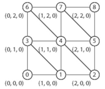
A kernel can find the global ID of the work-item it’s executing by calling get_global_id. In the example we saw yesterday the index space was unidimensional, and therefore the kernel only needed to call get_global_id once. Today we’ll create a kernel that multiplies two-dimensional matrices and therefore calls get_global_id twice.
Matrix Multiplication
First let’s take a quick detour to revisit the linear algebra we learned at school and remind ourselves how matrix multiplication works.
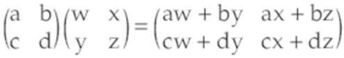
A matrix is a two-dimensional array of numbers. We can multiply a w×n matrix by an m×w matrix (note that the width of the first matrix must equal the height of the second) to get an m×n matrix. For example, multiplying a 2×4 matrix by a 3×2 matrix will give us a 3×4 result.
To calculate the value at (i, j) in the output matrix, we take the sum of multiplying every number in the jth row of the first matrix by the corresponding number in the ith column of the second matrix.
Here’s code that implements this sequentially:
|
|
#define WIDTH_OUTPUT WIDTH_B |
|
|
#define HEIGHT_OUTPUT HEIGHT_A |
|
|
|
|
|
float a[HEIGHT_A][WIDTH_A] = initialize a; |
|
|
float b[HEIGHT_B][WIDTH_B] = initialize b; |
|
|
float r[HEIGHT_OUTPUT][WIDTH_OUTPUT]; |
|
|
|
|
|
for (int j = 0; j < HEIGHT_OUTPUT; ++j) { |
|
|
for (int i = 0; i < WIDTH_OUTPUT; ++i) { |
|
|
float sum = 0.0; |
|
|
for (int k = 0; k < WIDTH_A; ++k) { |
|
|
sum += a[j][k] * b[k][i]; |
|
|
} |
|
|
r[j][i] = sum; |
|
|
} |
|
|
} |
As you can see, as the number of elements in our array increases, the work required to multiply them increases dramatically, making large-matrix multiplication a very CPU-intensive task indeed.
Parallel Matrix Multiplication
Here’s a kernel that can be used to multiply two-dimensional matrices:
|
DataParallelism/MatrixMultiplication/matrix_multiplication.cl |
|
|
Line 1 |
__kernel void matrix_multiplication(uint widthA, |
|
- |
__global const float* inputA, |
|
- |
__global const float* inputB, |
|
- |
__global float* output) { |
|
5 |
|
|
- |
int i = get_global_id(0); |
|
- |
int j = get_global_id(1); |
|
- |
|
|
- |
int outputWidth = get_global_size(0); |
|
10 |
int outputHeight = get_global_size(1); |
|
- |
int widthB = outputWidth; |
|
- |
|
|
- |
float total = 0.0; |
|
- |
for (int k = 0; k < widthA; ++k) { |
|
15 |
total += inputA[j * widthA + k] * inputB[k * widthB + i]; |
|
- |
} |
|
- |
output[j * outputWidth + i] = total; |
|
- |
} |
This kernel executes within a two-dimensional index space, each point of which identifies a location in the output array. It retrieves this point by calling get_global_id twice (lines 6 and 7).
It can find out the range of the index space by calling get_global_size, which this kernel uses to find the dimensions of the output matrix (lines 9 and 10). This also gives us widthB, which is equal to outputWidth, but we have to pass widthA as a parameter.
The loop on line 14 is just the inner loop from the sequential version we saw earlier—the only difference being that because OpenCL buffers are unidimensional, we can’t write the following:
|
|
output[j][i] = total; |
Instead, we have to use a little arithmetic to determine the correct offset:
|
|
output[j * outputWidth + i] = total; |
The host program required to execute this kernel is very similar to the one we saw yesterday, the only significant difference being the arguments passed to clEnqueueNDRangeKernel:
|
DataParallelism/MatrixMultiplication/matrix_multiplication.c |
|
|
|
size_t work_units[] = {WIDTH_OUTPUT, HEIGHT_OUTPUT}; |
|
|
CHECK_STATUS(clEnqueueNDRangeKernel(queue, kernel, 2, NULL, work_units, |
|
|
NULL, 0, NULL, NULL)); |
This creates a two-dimensional index space by setting work_dim to 2 (the third argument) and specifies the extent of each dimension by setting global_work_size to a two-element array (the fifth argument).
This kernel shows an even more dramatic performance benefit than the one we saw yesterday. On my MacBook Pro, multiplying a 200×400 matrix by a 300×200 matrix takes approximately 3 ms, compared to 66 ms on the CPU, a speedup of more than 20x.
Because this kernel is performing much more work per data element, we continue to see a significant speedup even if we take the overhead of copying data between the CPU and GPU into account. On my MacBook Pro, those copies take around 2 ms, for a total time of 5 ms, which still gives us a 13x speedup.
All the code we’ve run so far simply assumes that there’s an OpenCL-compatible GPU available. Clearly this may not always be true, so next let’s see how we can find out which OpenCL platforms and devices are available to a particular host.
Querying Device Info
OpenCL provides a number of functions that allow us to query the parameters of platforms, devices, and most other API objects. Here, for example, is a function that uses clGetDeviceInfo to query and print a device parameter with a value of type string:
|
DataParallelism/FindDevices/find_devices.c |
|
|
|
void print_device_param_string(cl_device_id device, |
|
|
cl_device_info param_id, |
|
|
const char* param_name) { |
|
|
char value[1024]; |
|
|
CHECK_STATUS(clGetDeviceInfo(device, param_id, sizeof(value), value, NULL)); |
|
|
printf("%s: %s\n", param_name, value); |
|
|
} |
Different parameters have values of different types (string, integer, array of size_t, and so on). Given a range of functions like the preceding, we can query the parameters of a particular device as follows:
|
DataParallelism/FindDevices/find_devices.c |
|
|
|
void print_device_info(cl_device_id device) { |
|
|
print_device_param_string(device, CL_DEVICE_NAME, "Name"); |
|
|
print_device_param_string(device, CL_DEVICE_VENDOR, "Vendor"); |
|
|
print_device_param_uint(device, CL_DEVICE_MAX_COMPUTE_UNITS, "Compute Units"); |
|
|
print_device_param_ulong(device, CL_DEVICE_GLOBAL_MEM_SIZE, "Global Memory"); |
|
|
print_device_param_ulong(device, CL_DEVICE_LOCAL_MEM_SIZE, "Local Memory"); |
|
|
print_device_param_sizet(device, CL_DEVICE_MAX_WORK_GROUP_SIZE, "Workgroup size"); |
|
|
} |
The code that accompanies this book includes a program called find_devices that uses this kind of code to query both the platforms and devices available. If I run it on my MacBook Pro, here’s what it prints:
|
|
Found 1 OpenCL platform(s) |
|
|
|
|
|
Platform 0 |
|
|
Name: Apple |
|
|
Vendor: Apple |
|
|
|
|
|
Found 2 device(s) |
|
|
|
|
|
Device 0 |
|
|
Name: Intel(R) Core(TM) i7-3720QM CPU @ 2.60GHz |
|
|
Vendor: Intel |
|
|
Compute Units: 8 |
|
|
Global Memory: 17179869184 |
|
|
Local Memory: 32768 |
|
|
Workgroup size: 1024 |
|
|
|
|
|
Device 1 |
|
|
Name: GeForce GT 650M |
|
|
Vendor: NVIDIA |
|
|
Compute Units: 2 |
|
|
Global Memory: 1073741824 |
|
|
Local Memory: 49152 |
|
|
Workgroup size: 1024 |
So there is a single platform available, the default Apple OpenCL implementation. Within that platform are two devices, the CPU and GPU.
There are a few interesting things we can see from this:
· OpenCL can target more than just GPUs (in addition to CPUs, it can also target dedicated OpenCL accelerators).
· The GPU in my MacBook Pro provides two compute units (we’ll see what a compute unit is soon).
· The GPU has 1 GiB of global memory.
· Each compute unit has 48 KiB of local memory and supports a maximum work-group size of 1024.
In the next sections, we’ll look at OpenCL’s platform and memory models and the implications they have for our code.
![]()
Joe asks:
Why Does OpenCL Target CPUs?
It comes as a surprise to many, but modern CPUs have long supported data-parallel instructions. Intel processors, for example, support the streaming SIMD extensions (SSE) and more recently the advanced vector extensions (AVX). OpenCL can provide an excellent way to exploit these instruction sets as well as the multiple cores that most CPUs now provide.
Platform Model
An OpenCL platform consists of a host that’s connected to one or more devices. Each device has one or more compute units, each of which provides a number of processing elements, as shown in Figure 14, The OpenCL Platform Model.
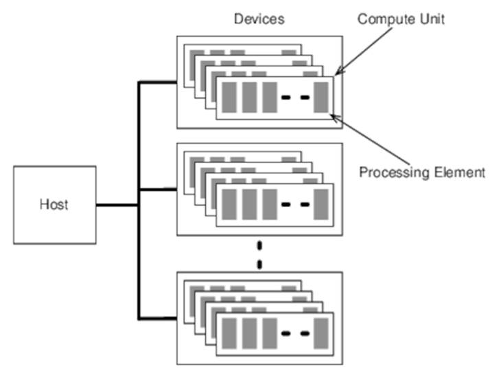
Figure 14. The OpenCL Platform Model
Work-items execute on processing elements. A collection of work-items executing on a single compute unit is a work-group. The work-items in a work-group share local memory, which brings us to OpenCL’s memory model.
Memory Model
A work-item executing a kernel has access to four different memory regions:
Global memory:
Memory available to all work-items executing on a device
Constant memory:
A region of global memory that remains constant during execution of a kernel
Local memory:
Memory local to a work-group; can be used for communication between work-items executing in that work-group (We’ll see an example of this soon.)
Private memory:
Memory private to a single work-item
![]()
Joe asks:
Is This How OpenCL Devices Actually Work?
The OpenCL platform and memory models don’t prescribe how the underlying hardware has to work. Instead they are abstractions of that hardware—different OpenCL devices have a range of different physical architectures.
For example, one OpenCL device might have local memory that really is local to a compute unit, whereas another might have local memory that in reality is mapped onto a region of global memory. Or one device might have its own distinct global memory, and another might have direct access to the host’s memory.
These architectural differences can have significant implications when it comes to optimizing OpenCL code, a subject that’s beyond the scope of this chapter.
As we’ve seen in previous chapters, a reduce operation over a collection can be a very effective approach to solving a wide range of problems. In the next section we’ll see how to implement a data-parallel reduce.
Data-Parallel Reduce
In this section we’ll create a kernel that finds the minimum element of a collection in parallel by reducing over that collection with the min operator.
Implementing this sequentially is straightforward:
|
DataParallelism/FindMinimumOneWorkGroup/find_minimum.c |
|
|
|
cl_float acc = FLT_MAX; |
|
|
for (int i = 0; i < NUM_VALUES; ++i) |
|
|
acc = fmin(acc, values[i]); |
We’ll see how to parallelize this in two steps—first with a single work-group and then with multiple work-groups.
A Single Work-Group Reduce
To make things simpler (we’ll see why this helps soon), I’m going to assume that the number of elements in the array we want to reduce is a power of two and small enough to be processed by a single work-group. Given that, here’s a kernel that will perform our reduce operation:
|
DataParallelism/FindMinimumOneWorkGroup/find_minimum.cl |
|
|
Line 1 |
__kernel void find_minimum(__global const float* values, |
|
- |
__global float* result, |
|
- |
__local float* scratch) { |
|
- |
int i = get_global_id(0); |
|
5 |
int n = get_global_size(0); |
|
- |
scratch[i] = values[i]; |
|
- |
barrier(CLK_LOCAL_MEM_FENCE); |
|
- |
for (int j = n / 2; j > 0; j /= 2) { |
|
- |
if (i < j) |
|
10 |
scratch[i] = min(scratch[i], scratch[i + j]); |
|
- |
barrier(CLK_LOCAL_MEM_FENCE); |
|
- |
} |
|
- |
if (i == 0) |
|
- |
*result = scratch[0]; |
|
15 |
} |
The algorithm has three distinct phases:
1. It copies the array from global to local (scratch) memory (line 6).
2. It performs the reduce (lines 8–12).
3. It copies the result to global memory (line 14).
The reduce operation proceeds by creating a reduce tree very similar to the one we saw when looking at Clojure’s reducers (see Divide and Conquer):
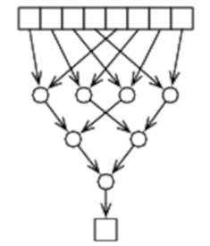
After each loop iteration, half the work-items become inactive—only work-items for which i < j is true perform any work (this is why we’re assuming that the number of elements in the array is a power of two—so we can repeatedly halve the array). The loop exits when only a single work-item is left active. Each active work-item performs a min between its value and the corresponding value in the remaining half of the array. By the time the loop exits, the first item in the scratch array will be the final value of the reduce operation, and the first work-item in the work-group copies this value to result.
The other interesting thing about this kernel is its use of barriers (lines 7 and 11) to synchronize access to local memory.
Barriers
A barrier is a synchronization mechanism that allows work-items to coordinate their use of local memory. If one work-item in a work-group executes barrier, then all work-items in that work-group must execute the same barrier before any of them can proceed beyond that point (a type of synchronization commonly known as a rendezvous). In our reduction kernel, this serves two purposes:
· It ensures that one work-item doesn’t start reducing until all work-items have copied their value from global to local memory and that one work-item doesn’t move on to loop iteration n + 1 until all work-items have finished loop iteration n.
· OpenCL only provides relaxed memory consistency. This is very similar to the Java Memory Model we saw in Memory Visibility—changes made to local memory by one work-item are not guaranteed visible to other work-items except at specific synchronization points, such as barriers. So executing a barrier at the end of each loop iteration guarantees that the results of iteration n are visible to the work-items executing iteration n + 1.
Executing the Kernel
Executing this kernel is very similar to what we’ve already seen—the only substantive new thing we need to worry about is how to create a local buffer:
|
DataParallelism/FindMinimumOneWorkGroup/find_minimum.c |
|
|
|
CHECK_STATUS(clSetKernelArg(kernel, 2, sizeof(cl_float) * NUM_VALUES, NULL)); |
We allocate a local buffer by calling clSetKernelArg with arg_size set to the size of the buffer we want to create and arg_value set to NULL.
A reduce that runs within a single work-group is great, but as we’ve seen, work-groups are restricted in size (no more than 1,024 elements on the GPU in my MacBook Pro, for example). Next, we’ll see how to parallelize over multiple work-groups.
A Multiple-Work-Group Reduce
Extending our reduce across multiple work-groups is a simple matter of dividing the input array into work-groups and reducing each independently, as shown in Figure 15, Extending the Reduce across Multiple Work-Groups.
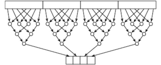
Figure 15. Extending the Reduce across Multiple Work-Groups
If, for example, each work-group operates on 64 values at a time, this will reduce an array of N items to N/64 items. This smaller array can then be reduced in turn, and so on, until only a single result remains.
Achieving this requires a few small changes to our kernel to allow it to operate on a work-group that represents a section of a larger problem. To this end, OpenCL provides work-items with a local ID, which is an ID just for within that work-group, as shown in Figure 16, The Local ID with a Work-Group.
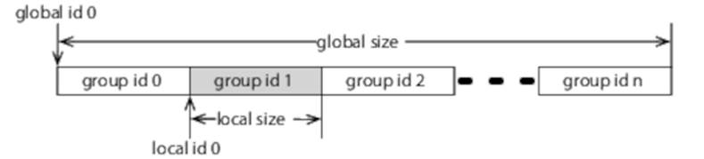
Figure 16. The Local ID with a Work-Group
Here’s a kernel that makes use of local IDs:
|
DataParallelism/FindMinimumMultipleWorkGroups/find_minimum.cl |
|
|
|
__kernel void find_minimum(__global const float* values, |
|
|
__global float* results, |
|
|
__local float* scratch) { |
|
* |
int i = get_local_id(0); |
|
* |
int n = get_local_size(0); |
|
* |
scratch[i] = values[get_global_id(0)]; |
|
|
barrier(CLK_LOCAL_MEM_FENCE); |
|
|
for (int j = n / 2; j > 0; j /= 2) { |
|
|
if (i < j) |
|
|
scratch[i] = min(scratch[i], scratch[i + j]); |
|
|
barrier(CLK_LOCAL_MEM_FENCE); |
|
|
} |
|
|
if (i == 0) |
|
* |
results[get_group_id(0)] = scratch[0]; |
|
|
} |
In place of get_global_id and get_global_size, we’re now calling get_local_id and get_local_size, which return the ID relative to the start of the work-group and size of the work-group, respectively. We still have to call get_global_id to copy the right value from global memory to local, andresults is now an array indexed by the get_group_id.
The final piece of this puzzle is to change the host program to create work-groups of the appropriate size:
|
DataParallelism/FindMinimumMultipleWorkGroups/find_minimum.c |
|
|
|
size_t work_units[] = {NUM_VALUES}; |
|
|
size_t workgroup_size[] = {WORKGROUP_SIZE}; |
|
|
CHECK_STATUS(clEnqueueNDRangeKernel(queue, kernel, 1, NULL, work_units, |
|
|
workgroup_size, 0, NULL, NULL)); |
If we set local_work_size to NULL, as we have been doing up to now, the OpenCL platform is free to create work-groups of whatever size it sees fit. By explicitly setting local_work_size, we guarantee that work-groups are the size required by our kernel (up to the maximum size supported by the device, of course—see Querying Device Info, to determine how to find this).
Day 2 Wrap-Up
This brings us to the end of day 2. In day 3 we’ll see an example of an application that implements a physics simulation with OpenCL and integrates with OpenGL to display the results.
What We Learned in Day 2
OpenCL defines platform, execution, and memory models that abstract the details of the underlying hardware.
· Work-items execute on processing elements.
· Processing elements are grouped into compute units.
· A group of work-items executing on a single compute unit is a work-group.
· Work-items in a work-group communicate through local memory using barriers to synchronize and ensure consistency.
Day 2 Self-Study
Find
· By default, a command queue processes commands in order. How do you enable out-of-order execution?
· What is an event wait list? How might you use event wait lists to impose constraints on when commands sent to an unordered command queue are executed?
· What does clEnqueueBarrier do? When might you use barriers and when might you use wait lists?
Do
· Extend the reduce example to handle any number of elements, not just powers of two.
· Modify the reduce example to target multiple devices. If you have only a single OpenCL-compatible device, you can target the CPU as well, or you can partition your GPU with clCreateSubDevices. You will need to create a command queue for each device, partition the problem so that some work-items are executed on one device and some on the other, and synchronize between the command queues.
· The reduce algorithm we looked at today is very simple. An Internet search will uncover many approaches to creating a more efficient reduce. How fast can you get it on your particular device? Do the optimizations that work best on your GPU also work effectively on the CPU?
Day 3: OpenCL and OpenGL—Keeping It on the GPU
Today we’ll put together a complete OpenCL application that both runs and visualizes a simple physics simulation. In the process, we’ll see not only how to create a kernel that executes the simulation in parallel but also how to integrate OpenCL with OpenGL and avoid the overhead of buffer copies by keeping everything on the GPU.
Water Ripples
The simulation we’re going to create is of water ripples. It’s not going to be a hyperaccurate physical simulation, but it will be good enough to look convincing as a graphical effect in a game—to simulate, for example, the surface of a pond during a rain shower.
LWJGL
We’re going to move away from C for this example and instead use Java together with the Lightweight Java Graphics Library (LWJGL),[50] because that makes creating a cross-platform GUI easier.
LWJGL provides Java wrappers for both OpenCL and OpenGL, allowing a Java program to access OpenGL and OpenCL’s C APIs. As OpenGL’s name suggests, it has close ties with OpenCL. In particular, as we’ll see later, it’s possible for an OpenCL kernel executing on the GPU to directly operate on OpenGL buffers.
OpenCL code in LWJGL looks very similar to what we’ve already seen in C. Here, for example, is code to initialize an OpenCL context, queue, and kernel:
|
DataParallelism/Zoom/src/main/java/com/paulbutcher/Zoom.java |
|
|
|
CL.create(); |
|
|
CLPlatform platform = CLPlatform.getPlatforms().get(0); |
|
|
List<CLDevice> devices = platform.getDevices(CL_DEVICE_TYPE_GPU); |
|
|
CLContext context = CLContext.create(platform, devices, null, drawable, null); |
|
|
CLCommandQueue queue = clCreateCommandQueue(context, devices.get(0), 0, null); |
|
|
|
|
|
CLProgram program = |
|
|
clCreateProgramWithSource(context, loadSource("zoom.cl"), null); |
|
|
Util.checkCLError(clBuildProgram(program, devices.get(0), "", null)); |
|
|
CLKernel kernel = clCreateKernel(program, "zoom", null); |
As you can see, both the method names and arguments are almost identical to the equivalent C code. The few small changes are necessary to handle differences between the languages, such as the absence of pointers in Java, but broadly speaking it’s possible to transliterate an OpenGL host program written in C to Java with LWJGL.
Displaying a Mesh in OpenGL
We’re not going to spend much time talking about the OpenGL element of this example. But we do need to spend a little time understanding how our example displays the mesh that represents the water surface so that we know the task that faces our OpenCL code.
An OpenGL 3D scene is constructed from triangles. In our case, we’re creating a mesh out of triangles arranged like this:
We specify the position of each triangle with two steps—a vertex buffer that defines a set of vertices (points in 3D space) and an index buffer that defines which of those vertices are used to draw each triangle.
So in the preceding example, vertex 0 is at (0, 0, 0), vertex 1 is at (1, 0, 0), vertex 2 is at (2, 0, 0), and so on. The vertex buffer will therefore contain [0, 0, 0, 1, 0, 0, 2, 0, 0, 0, 1, 0, 1, 1, 0, …].
As for the index buffer, the first triangle will use vertices 0, 1, and 3; the second 1, 3, and 4; the third 1, 2, and 4; and so on. The index buffer we create defines a triangle strip in which, after specifying the first triangle with three vertices, we only need a single additional vertex to define the next triangle:
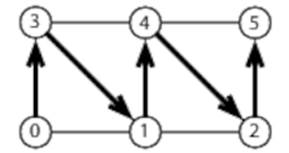
So our index buffer will contain [0, 3, 1, 4, 2, 5, …].
The code that accompanies this book includes a Mesh class that generates initial values for the vertex and index buffers. Our sample uses this to create a 64×64 mesh with x- and y-coordinates ranging from -1.0 to 1.0:
|
DataParallelism/Zoom/src/main/java/com/paulbutcher/Zoom.java |
|
|
|
Mesh mesh = new Mesh(2.0f, 2.0f, 64, 64); |
The z-coordinates are all initialized to zero—we’ll modify them during animation to simulate ripples.
This data is then copied to OpenGL buffers as follows:
|
DataParallelism/Zoom/src/main/java/com/paulbutcher/Zoom.java |
|
|
|
int vertexBuffer = glGenBuffers(); |
|
|
glBindBuffer(GL_ARRAY_BUFFER, vertexBuffer); |
|
|
glBufferData(GL_ARRAY_BUFFER, mesh.vertices, GL_DYNAMIC_DRAW); |
|
|
|
|
|
int indexBuffer = glGenBuffers(); |
|
|
glBindBuffer(GL_ELEMENT_ARRAY_BUFFER, indexBuffer); |
|
|
glBufferData(GL_ELEMENT_ARRAY_BUFFER, mesh.indices, GL_STATIC_DRAW); |
Each buffer has an ID allocated by glGenBuffers, is bound to a target with glBindBuffer, and has its initial values set with glBufferData. The index buffer has the GL_STATIC_DRAW usage hint, indicating that it won’t change (is static). The vertex buffer, by contrast, has theGL_DYNAMIC_DRAW hint because it will change between animation frames.
Before we implement the ripple code, we’ll start with something easier—a simple kernel that increases the size of the mesh over time.
Accessing an OpenGL Buffer from an OpenCL Kernel
Here’s the kernel that implements our zoom animation:
|
DataParallelism/Zoom/src/main/resources/zoom.cl |
|
|
|
__kernel void zoom(__global float* vertices) { |
|
|
|
|
|
unsigned int id = get_global_id(0); |
|
|
vertices[id] *= 1.01; |
|
|
} |
It takes the vertex buffer as an argument and multiplies every entry in that buffer by 1.01, increasing the size of the mesh by 1% every time it’s called.
Before we can pass the vertex buffer to our kernel, we first need to create an OpenCL buffer that references it:
|
DataParallelism/Zoom/src/main/java/com/paulbutcher/Zoom.java |
|
|
|
CLMem vertexBufferCL = |
|
|
clCreateFromGLBuffer(context, CL_MEM_READ_WRITE, vertexBuffer, null); |
This buffer object can then be used in our main rendering loop as follows:
|
DataParallelism/Zoom/src/main/java/com/paulbutcher/Zoom.java |
|
|
|
while (!Display.isCloseRequested()) { |
|
|
glClear(GL_COLOR_BUFFER_BIT | GL_DEPTH_BUFFER_BIT); |
|
|
glLoadIdentity(); |
|
|
glTranslatef(0.0f, 0.0f, planeDistance); |
|
|
glDrawElements(GL_TRIANGLE_STRIP, mesh.indexCount, GL_UNSIGNED_SHORT, 0); |
|
|
|
|
|
Display.update(); |
|
|
|
|
* |
Util.checkCLError(clEnqueueAcquireGLObjects(queue, vertexBufferCL, null, null)); |
|
* |
kernel.setArg(0, vertexBufferCL); |
|
* |
clEnqueueNDRangeKernel(queue, kernel, 1, null, workSize, null, null, null); |
|
* |
Util.checkCLError(clEnqueueReleaseGLObjects(queue, vertexBufferCL, null, null)); |
|
* |
clFinish(queue); |
|
|
} |
Before an OpenCL kernel can use an OpenGL buffer, we need to acquire it with clEnqueueAcquireGLObjects. We can then set it as an argument to our kernel and call clEnqueueNDRangeKernel as normal. Finally, we release the buffer with clEnqueueReleaseGLObjects and wait for the commands we’ve dispatched to finish with clFinish.
Run this code, and you should see the mesh start out small and quickly grow to the point that a single triangle fills the screen.
Now that we’ve got a simple animation working that integrates OpenGL with OpenCL, we’ll look at the more sophisticated kernel that implements our water ripples.
Simulating Ripples
We’re going to simulate expanding rings of ripples. Each expanding ring is defined by a 2D point on the mesh (the center of the expanding ring) together with a time (the time at which the ring started expanding). As well as taking a pointer to the OpenGL vertex buffer, our kernel takes an array of ripple centers together with a corresponding array of times (where time is measured in milliseconds):
|
DataParallelism/Ripple/src/main/resources/ripple.cl |
|
|
Line 1 |
#define AMPLITUDE 0.1 |
|
- |
#define FREQUENCY 10.0 |
|
- |
#define SPEED 0.5 |
|
- |
#define WAVE_PACKET 50.0 |
|
5 |
#define DECAY_RATE 2.0 |
|
- |
__kernel void ripple(__global float* vertices, |
|
- |
__global float* centers, |
|
- |
__global long* times, |
|
- |
int num_centers, |
|
10 |
long now) { |
|
- |
unsigned int id = get_global_id(0); |
|
- |
unsigned int offset = id * 3; |
|
- |
float x = vertices[offset]; |
|
- |
float y = vertices[offset + 1]; |
|
15 |
float z = 0.0; |
|
- |
|
|
- |
for (int i = 0; i < num_centers; ++i) { |
|
- |
if (times[i] != 0) { |
|
- |
float dx = x - centers[i * 2]; |
|
20 |
float dy = y - centers[i * 2 + 1]; |
|
- |
float d = sqrt(dx * dx + dy * dy); |
|
- |
float elapsed = (now - times[i]) / 1000.0; |
|
- |
float r = elapsed * SPEED; |
|
- |
float delta = r - d; |
|
25 |
z += AMPLITUDE * |
|
- |
exp(-DECAY_RATE * r * r) * |
|
- |
exp(-WAVE_PACKET * delta * delta) * |
|
- |
cos(FREQUENCY * M_PI_F * delta); |
|
- |
} |
|
30 |
} |
|
- |
vertices[offset + 2] = z; |
|
- |
} |
We start by determining the x- and y-coordinates of the vertex that’s being processed by the current work-item (lines 13 and 14). In the loop (lines 17–30) we calculate a new z-coordinate that we write back to the vertex buffer on line 31.
Within the loop, we examine each ripple center with a nonzero start time in turn. For each, we start by determining the distance d between the point we’re calculating and the ripple center (line 21). Next, we calculate the radius r of the expanding ripple ring (line 23) and δ, the distance between our point and this ripple ring (line 24):
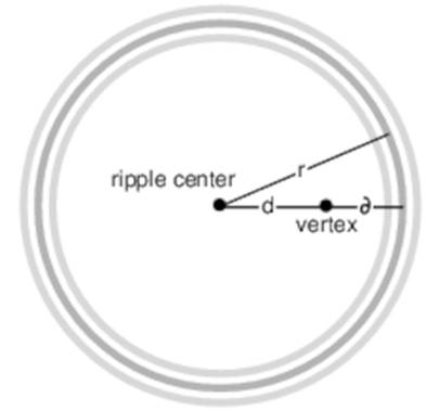
Finally, we can combine δ and r to get z:
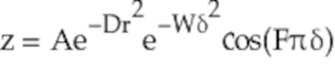
Here, A, D, W, and F are constants representing the amplitude of the wave packet, the rate at which it decays as it expands, the width of the wave packet, and the frequency, respectively.
The final piece of the puzzle is to extend our host application to create our ripple centers:
|
DataParallelism/Ripple/src/main/java/com/paulbutcher/Ripple.java |
|
|
|
int numCenters = 16; |
|
|
int currentCenter = 0; |
|
|
FloatBuffer centers = BufferUtils.createFloatBuffer(numCenters * 2); |
|
|
centers.put(new float[numCenters * 2]); |
|
|
centers.flip(); |
|
|
LongBuffer times = BufferUtils.createLongBuffer(numCenters); |
|
|
times.put(new long[numCenters]); |
|
|
times.flip(); |
|
|
|
|
|
CLMem centersBuffer = |
|
|
clCreateBuffer(context, CL_MEM_READ_ONLY | CL_MEM_COPY_HOST_PTR,centers, null); |
|
|
CLMem timesBuffer = |
|
|
clCreateBuffer(context, CL_MEM_READ_ONLY | CL_MEM_COPY_HOST_PTR, times, null); |
And start a new ripple whenever the mouse is clicked:
|
DataParallelism/Ripple/src/main/java/com/paulbutcher/Ripple.java |
|
|
|
while (Mouse.next()) { |
|
|
if (Mouse.getEventButtonState()) { |
|
|
float x = ((float)Mouse.getEventX() / Display.getWidth()) * 2 - 1; |
|
|
float y = ((float)Mouse.getEventY() / Display.getHeight()) * 2 - 1; |
|
|
|
|
|
FloatBuffer center = BufferUtils.createFloatBuffer(2); |
|
|
center.put(new float[] {x, y}); |
|
|
center.flip(); |
|
|
clEnqueueWriteBuffer(queue, centersBuffer, 0, |
|
|
currentCenter * 2 * FLOAT_SIZE, center, null, null); |
|
|
LongBuffer time = BufferUtils.createLongBuffer(1); |
|
|
time.put(System.currentTimeMillis()); |
|
|
time.flip(); |
|
|
|
|
|
clEnqueueWriteBuffer(queue, timesBuffer, 0, |
|
|
currentCenter * LONG_SIZE, time, null, null); |
|
|
currentCenter = (currentCenter + 1) % numCenters; |
|
|
} |
|
|
} |
Compile and run this code, click on the mesh a few times, and you should see something like Figure 17, Ripples.
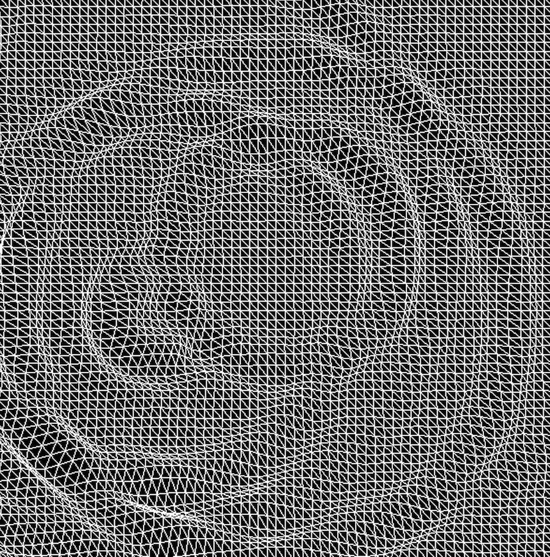
Figure 17. Ripples
So there we have it—we’ve created a physical simulation in which both the calculations to perform the simulation and the 3D visualization of the results are carried out on the GPU in parallel. All the data necessary to perform both the calculation and the visualization resides permanently on the GPU, no copying required.
Day 3 Wrap-Up
That brings us to the end of day 3 and our discussion of data parallelism on the GPU via OpenCL.
What We Learned in Day 3
An OpenCL kernel running on a GPU can directly access buffers used by an OpenGL application running on the same GPU. We covered how to do the following:
· Create an OpenCL view of an OpenGL buffer with clCreateFromGLBuffer
· Acquire an OpenGL buffer before passing it to a kernel with clEnqueueAcquireGLObjects
· Release the buffer after the kernel has finished with clEnqueueReleaseGLObjects
Day 3 Self-Study
Find
· What is an image object? How does it differ from an ordinary OpenCL buffer? Do image objects have use cases in kernels that don’t interoperate with OpenGL?
· What is a sampler object? What problems can it help solve?
· What are atomic functions? When might you use atomic functions instead of barriers?
Do
· Without using atomic functions, create a kernel that takes a buffer of integers with values between 0 and 32 and implements a histogram by counting how many instances of each value there are in the buffer. Can you extend your solution to do the same for a buffer that contains values between 0 and 1024?
· Write a kernel to perform the same task as above but using atomic functions this time. How do the two solutions compare?
Wrap-Up
For some reason, data parallelism seems to be ignored in many mainstream discussions of parallelism. As you can see, however, it’s an extremely powerful way to dramatically improve your code’s performance and one that all programmers should have in their repertoire.
Strengths
Data parallelism is ideal whenever you’re faced with a problem where large amounts of numerical data needs to be processed. It’s particularly appropriate for scientific and engineering computing and for simulation. Examples include fluid dynamics, finite element analysis, n-body simulation, simulated annealing, ant-colony optimization, neural networks, and so on.
GPUS are not only powerful data-parallel processors; they are also extremely efficient in their power consumption, typically returning much better GFLOPS/watt results than a traditional CPU. This is one of the primary reasons why many of the fastest supercomputers in the world make extensive use of either GPUs or dedicated data-parallel coprocessors.[51]
Weaknesses
Within its niche, data-parallel programming in general, and GPGPU programming specifically, is hard to beat. But it’s not an approach that lends itself to all problems. In particular, although it is possible to use these techniques to create solutions to nonnumerical problems (natural language processing, for example), doing so is not straightforward—the current toolset is very much focused on number-crunching.
Optimizing an OpenCL kernel can be tricky, and effective optimization often depends on understanding underlying architectural details. This can be a particular issue if you need to write high-performance cross-platform code. For some problems, the need to copy data from the host to the device can dominate execution time, negating or reducing the benefit to be gained from parallelizing the computation.
Other Languages
Other GPGPU frameworks include CUDA,[52] DirectCompute,[53] and RenderScript Computation.[54]
Final Thoughts
GPGPU programming is an example of data parallelism in the small—on a single machine. In the next chapter we’ll look at the Lambda Architecture, which allows us to exploit data parallelism in the large—across multiple machines.
Footnotes
|
[48] |
http://www.khronos.org/opencl/ |
|
[49] |
http://www.opengl.org |
|
[50] |
http://www.lwjgl.org |
|
[51] |
http://www.top500.org/lists/2013/06/ |
|
[52] |
http://www.nvidia.com/object/cuda_home_new.html |
|
[53] |
http://msdn.com/directx |
|
[54] |
http://developer.android.com/guide/topics/renderscript/compute.html |