Programming Google App Engine with Python (2015)

Chapter 7. Datastore Queries

Inevitably, an application that manages data must do more than store and retrieve that data one record at a time. It must also answer questions about that data: which records meet certain criteria, how records compare to one another, what a set of records represents in aggregate. Web applications in particular are expected not only to know the answers to questions about large amounts of data, but to provide them quickly in response to web requests.

Most database systems provide a mechanism for executing queries, and Cloud Datastore is no exception. But the datastore’s technique differs significantly from that of traditional database systems. When the application asks a question, instead of rifling through the original records and performing calculations to determine the answer, Cloud Datastore simply finds the answer in a list of possible answers prepared in advance. The datastore can do this because it knows which questions are going to be asked.

This kind of list, or index, is common to many database technologies, and relational databases can be told to maintain a limited set of indexes to speed up some kinds of queries. But Cloud Datastore is different: it maintains an index for every query the application is going to perform. Because the datastore only needs to do a simple scan of an index for every query, the application gets results back quickly. And for large amounts of data, Cloud Datastore can spread the data and the indexes across many machines, and get results back from all of them without an expensive aggregateoperation.

This indexing strategy has significant drawbacks. The datastore’s built-in query engine is downright weak compared to some relational databases, and is not suited to sophisticated data processing applications that would prefer slow but powerful runtime queries to fast simple ones. But most web applications need fast results, and the dirty secret about those powerful query engines is that they can’t perform at web speeds with large amounts of data distributed across many machines. Cloud Datastore uses a model suited to scalable web applications: calculate the answers to known questions when the data is written, so reading is fast.

In this chapter, we explain how queries and indexes work, how the developer tools help you configure indexes automatically, and how to manage indexes as your application evolves. We also discuss several powerful features of the query engine, including cursors and projection queries. By understanding indexes, you will have an intuition for how to design your application and your data to make the most of the scalable datastore.

Queries and Kinds

You’ve seen how to retrieve an entity from the datastore given its key. But in most cases, the application does not know the keys of the entities it needs; it has only a general idea that it needs entities that meet certain criteria. For example, a leaderboard for the game app would need to retrieve the 10 Player entities with the highest score property values.

To retrieve entities this way, the app performs a query. A query includes:

§ The kind of the entities to query

§ Zero or more filters, criteria that property values must meet for an entity to be returned by the query

§ Zero or more sort orders that determine the order in which results are returned based on property values

A query based on property values can only return entities of a single kind. This is the primary purpose of kinds: to determine which entities are considered together as possible results for a query. In practice, kinds correspond to the intuitive notion that each entity of the same nominal kind represents the same kind of data. But unlike other database systems, it’s up to the app to enforce this consistency if it is desired, and the app can diverge from it if it’s useful.

It is also possible to perform a limited set of queries on entities regardless of kind. Kindless queries can use a filter on the ID or key name, or on ancestors. We’ll discuss ancestors and kindless queries in Chapter 8.

Query Results and Keys

When retrieving results for an entity query, the datastore returns the full entity for each result to the application.

For large entities, this may mean more data is transmitted between the datastore and the app than is needed. It’s possible to fetch only a subset of properties under certain circumstances (we’ll see this in “Projection Queries”), but these are not full entities. Another option is to store frequently accessed properties on one entity, and less popular properties on a separate related entity. The first entity stores the key of the second entity as a property, so when the app needs the less popular data, it queries for the first entity, then follows the reference to the second entity.

The datastore can return just the keys for the entities that match your query instead of fetching the full entities. A keys-only query is useful for determining the entities that match query criteria separately from when the entities are used. Keys can be remembered in the memcache or in a datastore property, and vivified as full entities when needed. We’ll look at the API for keys-only queries a bit later.

The Query API

Recall that the Python datastore API represents entities using objects of classes named after kinds. To review, here is code that creates three Player entities for an online role-playing game:

from google.appengine.ext import ndb

import datetime

class Player(ndb.Model):

name = ndb.StringProperty()

level = ndb.IntegerProperty()

score = ndb.IntegerProperty()

charclass = ndb.StringProperty()

create_date = ndb.DateTimeProperty(auto_now_add=True)

player1 = Player(name='wizard612',

level=1,

score=32,

charclass='mage')

player1.put()

player2 = Player(name='druidjane',

level=10,

score=896,

charclass='druid')

player2.put()

player3 = Player(name='TheHulk',

level=7,

score=500,

charclass='warrior')

player3.put()

This example uses the Model base class and declared property types. Declared properties help to enforce a consistent layout, or schema, for your entities. As we start talking about queries, the importance of using a schema for entities of a kind will become apparent.

Here is a simple query for entities of the Player kind that have a level property greater than or equal to 5:

q = Player.query().filter(Player.level >= 5)

results = q.fetch(10)

for entity inresults:

# assert entity.level >= 5

# ...

WARNING

When you create or update an entity with new data, the indexes that support queries about that data are also updated. For the type of queries discussed in this chapter, the call to put() may return before the indexes have been updated. If you perform such a query immediately after an update, the results may not reflect the change. The development server simulates this possibility with a delay:

player1.level = 6

player1.put()

# put() returns while the Player.level

# index update is still in progress.

q = Player.query().filter(Player.level >= 5)

results = q.fetch(10)

# results may not contain player1.

We’ll discuss consistency guarantees and how to formulate queries transactionally in Chapter 8.

The API provides two ways to formulate queries, one using an object-oriented interface, and one based on a text-based query language called “GQL.”

The Query Class

The first way to formulate a query is with an instance of the Query class. The Query object can be constructed in one of two ways, with equivalent results:

q = Player.query()

q = ndb.Query(kind=Player)

In both cases, q is assigned a new Query instance that represents all entities of the kind Player. The query is not executed right away; right now it’s just a question waiting to be asked. Without filters or sort orders, the object represents a query for all objects of the given kind.

To apply a filter to the query, you call the filter() method on the Query object. This returns a new Query object, leaving the original object unchanged.1 The argument to the filter() method is an expression that describes the filter, consisting of a property, an operator, and a value:

q = q.filter(Player.level > 5)

Yes, this looks a little weird, but it actually does what it looks like it does. The property is described using the attribute of the model class that functions as the property declaration (Player.level). With a little Python magic, applying the comparison operator and value to this attribute results in a filter expression that the filter() method understands. By referring to the class attribute directly in the code, ndb provides a bit of code safety, validating that you’re using a real model class, a declared attribute, and the correct value type.

You specify multiple filters by calling the filter() method multiple times. An entity must meet all filter criteria in order to be a result for the query. That is, filters have a logical AND relationship with one another:

q = q.filter(Player.level > 5)

q = q.filter(Player.level < 20)

For convenience, the filter() method returns the Query object, so you can chain multiple calls to filter() in a single line:

q = q.filter(Player.level > 5).filter(Player.level < 20)

The filter() method supports the equality (==) operator and the four inequality operators (<, <=, >, and >=). The Query class also supports the != (not equal) and IN operators. These are not primitive datastore query operators: instead, the query library executes these operators by performing multiple datastore queries then aggregating the results.

To apply a sort order, you call the order() method. As with filter(), this returns a new Query object derived from the original. This method takes one argument, the property to sort by, in the form of a reference to the class attribute. By default, the sort will be in ascending order. To sort by the property in descending order, use the unary negation operator on the property:

q = q.order(Player.level)

q = q.order(-Player.score)

The datastore can sort query results by multiple properties. First, it sorts by the property and order from the first call to order(), then it sorts entities with equal values for the first property, using the second order, and so on. For example, the following sorts first by level ascending, then byscore descending:

q = q.order(Player.level).order(-Player.score)

The query engine supports limiting the number of results returned, and skipping ahead a number of results. You specify the limit and offset when you retrieve the results, described later.

TIP

The property name used in an ndb filter or sort order expression refers to the property declaration stored as an attribute of the model class. When using the ndb.Expando base class, you can have properties on an entity that are not declared in this way. To refer to these properties in a filter or sort order expression, you can instantiate a temporary declaration using thendb.GenericProperty() constructor:

class Document(ndb.Expando):

pass

# ...

q = Document.query()

q = q.filter(ndb.GenericProperty('category')

== 'biology')

AND and OR clauses

Setting multiple filters on a Query object is logically equivalent to combining each of the filters with a logical AND operator. You can state this more explicitly in the API using the ndb.AND() combination:

q = Player.query()

q = q.filter(Player.level > 5)

q = q.filter(Player.level < 20)

q = Player.query(ndb.AND(Player.level > 5,

Player.level < 20))

The ndb.AND() function takes two clauses. Either of these clauses can be another ndb.AND() expression.

This is mostly useful when combined with the ndb.OR() function, which forms a logical OR relationship between two clauses:

q = Player.query(ndb.OR(ndb.AND(Player.level > 5,

Player.level < 20),

ndb.AND(Player.charclass == 'mage'),

Player.level > 3))

This query asks for Player entities that either have a level between 5 and 20, or are of a character class of 'mage' and have a level greater than 3.

The datastore does not support logical OR natively. Instead, ndb normalizes the total logical expression into a form that can be expressed as multiple primitive queries that use only logical AND operators. It then makes multiple calls to the datastore and aggregates the results.

Notice that complex logical expressions may require many primitive datastore queries to perform. This can impact performance. Nevertheless, ndb.OR() is sometimes convenient.

GQL

ndb also supports a more succinct way to formulate queries: a text-based query language called GQL. This language is intended to resemble SQL, the query language of relational databases. It supports only the features of the datastore’s query engine, and therefore lacks many features common to SQL. But it is expressive and concise enough to be useful for datastore queries.

Say we have entities of the kind Player representing players in an online role-playing game. The following GQL query retrieves all Player entities whose “level” property is an integer between 5 and 20, sorted by level in ascending order, then by score in descending order:

SELECT * FROM Player

WHERE level >= 5

AND level <= 20

ORDER BY level ASC, score DESC

In Python code, you create the query object from a GQL statement using the ndb.gql() function:

q = ndb.gql("""SELECT * FROM Player

WHERE level > 5

AND level < 20

ORDER BY level ASC, score DESC""")

Alternatively, you can call the gql() method on the model class, omitting the SELECT * FROM Kind from the string as this is implied by the use of the method:

q = Player.gql("""WHERE level > 5

AND level < 20

ORDER BY level ASC, score DESC""")

The first part of the SQL-like syntax in the preceding GQL query, SELECT * FROM Player, says that the datastore should return complete entities as results, and that it should only consider entities of the kind Player. This is the most common kind of query. Unlike a SQL database, the datastore cannot “join” properties from entities of multiple kinds into a single set of results. Only one kind can appear after the FROM.

Despite its similarity with SQL, GQL can only represent queries, and cannot perform updates, inserts, or deletes. In other words, every GQL query begins with SELECT.

The rest of the query syntax also resembles SQL, and translates directly to filters and sort orders. The WHERE clause, if present, represents one or more filter conditions, separated by AND. The ORDER BY clause, if present, represents one or more sort orders, separated by commas, applied from left to right.

Each condition in a WHERE clause consists of the name of a property, a comparison operator, and a value. You can also specify a condition that matches an entity’s ID or key name by using the reserved name __key__ like a property name. (That’s two underscores, the word “key,” and two underscores.)

The datastore query engine supports five comparison operators for filters: =, <, <=, >, and >=. GQL also supports two additional operators: !=, meaning “not equal to,” and IN, which tests that the value equals any in a set of values.

TIP

With ndb, the equality operator is the Python equality operator: Player.level == 5. In GQL, the equality operator is a single = similar to SQL: SELECT * FROM Player WHERE level = 5.

For IN, the values are represented by a comma-delimited list of values surrounded by parentheses:

SELECT * FROM Player WHERE level IN (5, 6, 7)

Internally, GQL translates the != and IN operators into multiple datastore queries that have the same effect. If a query contains an IN clause, the query is evaluated once for each value in the clause, using an = filter. The results of all the queries are aggregated. The != operator performs the query once using a < filter and once using a >, then aggregates the results. Using these operators more than once in a GQL statement requires a query for each combination of the required queries, so be judicious in their use.

The WHERE clause is equivalent to one or more filters. It is not like SQL’s WHERE clause, and does not support arbitrary logical expressions. In particular, GQL does not support testing the logical OR of two conditions.

The value on the righthand side of a condition can be a literal value that appears inside the query string. Seven of the datastore value types have string literal representations, as shown in Table 7-1.

The type of a filter’s value is significant in a datastore query. If you use the wrong type for a value, such as by specifying a 'string_key' when you meant to specify a KEY(kind, key_name), your query may not return the results you intend, or may unexpectedly return no results.

A GQL query can specify a LIMIT, a maximum number of results to return. A query can also specify an OFFSET, a number of results to skip before returning the remaining results. The following example returns the third, fourth, and fifth results, and may return fewer if the query has fewer than five results:

SELECT * FROM Player LIMIT 3 OFFSET 2

GQL keywords, shown here in uppercase, are case insensitive. Kind and property names, however, are case sensitive.

As with SQL statements in code, it is not always safe to include query values directly in the query string, especially if those values come from outside sources. You don’t want values to be accidentally (or maliciously) mistaken for GQL syntax characters. This is less of an issue for GQL than for SQL (since GQL statements can only perform queries and cannot modify data) but it’s still good practice to isolate values from the query string.

To specify values separately from the query string, you use parameter substitution. With parameter substitution, the query string contains a placeholder with either a number or a name, and the actual value is passed to gql() as either a positional argument or a keyword argument. The number or name appears in the query string preceded by a colon (:1 or :argname):

q = ndb.gql("""SELECT * FROM Player

WHERE level > :1

AND level < :2""",

5, 20)

q = ndb.gql("""SELECT * FROM Player

WHERE level > :min_level

AND level < :max_level""",

min_level=5, max_level=20)

One advantage to parameter substitution is that each argument value is of the appropriate datastore type, so you don’t need to bother with the string syntax for specifying typed values.

You can rebind new values to a GQL query by using parameter substitution after the query object has been instantiated using the bind() method. This means you can reuse the query multiple times for different values. This saves time because the query string only needs to be parsed once. The bind() method takes the new values as either positional arguments or keyword arguments, and returns a new query object with parameters bound.

You can save more time by caching parameterized query objects in global variables. This way, the query string is parsed only when a server loads the application for the first time, and the application reuses the object for all subsequent calls handled by that server:

_LEADERBOARD_QUERY = ndb.gql(

"""SELECT * FROM Player

WHERE level > :min_level

AND level < :max_level

ORDER BY level ASC, score DESC""")

class LeaderboardHandler(webapp.RequestHandler):

def get(self):

q = _LEADERBOARD_QUERY.bind(min_level=5, max_level=20)

# ...

TIP

You can use GQL to perform queries from the Cloud Console. In the sidebar, expand Storage, Cloud Datastore, Query. Locate the dropdown menu that reads “Query by kind,” then change it to “Query using GQL.” Enter the GQL statement, then click the Run button to run it.

Note that to perform a query in the Console, the app must already have an index that corresponds to the query. We’ll discuss indexes throughout this chapter.

Retrieving Results

Once you have a query object configured with filters, sort orders, and value bindings (in the case of GQL), you can execute the query, using one of several methods. The query is not executed until you call one of these methods, and you can call these methods repeatedly on the same query object to re-execute the query and get new results.

The fetch() method returns a number of results, up to a specified limit. fetch() returns a list of entity objects, which are instances of the kind class:

q = ndb.Player.query().order(-Player.score)

results = q.fetch(10)

When serving web requests, it’s always good to limit the amount of data the datastore might return, so an unexpectedly large result set doesn’t cause the request handler to exceed its deadline. The fetch() method requires an argument specifying the number of results to fetch (the limitargument).

The fetch() method also accepts an optional offset parameter. If provided, the method skips that many results, then returns subsequent results, up to the specified limit:

q = ndb.Player.query().order(-Player.score)

results = q.fetch(10, offset=20)

With GQL, the fetch result limit and offset are equivalent to the LIMIT and OFFSET that can be specified in the query string itself. The arguments to fetch() override those specified in the GQL statement. The limit argument to fetch() is required, so it always overrides a GQL LIMITclause.

NOTE

In order to perform a fetch with an offset, the datastore must find the first result for the query and then scan down the index to the offset. The amount of time this takes is proportional to the size of the offset, and may not be suitable for large offsets.

If you just want to retrieve results in batches, such as for a paginated display, there’s a better way: query cursors. For information on cursors, see “Query Cursors”.

It’s common for an app to perform a query expecting to get just one result, or nothing. You can do this with fetch(1), and then test whether the list it returns is empty. For convenience, the query object also provides a get() method, which returns either the first result, or None if the query did not return any results:

q = ndb.Player.query().filter(Player.name == 'django97')

player = q.get()

if player:

# ...

The count() method executes the query, then returns the number of results that would be returned instead of the results themselves. count() must perform the query to count the results in the index, and so takes time proportional to what it is counting. count() accepts a limit as a parameter, and providing one causes the method to return immediately once that many results have been counted:

q = ndb.Player.query().filter(Player.level > 10)

if q.count(100) == 100:

# 100 or more players are above level 10.

TIP

To test whether a query would return a result, without retrieving any results:

if q.count(1) == 1:

# The query has at least one result.

Query objects provide one other mechanism for retrieving results, and it’s quite powerful. In the Python API, query objects are iterable. If you use the object in a context that accepts iterables, such as in a for loop, the object executes the query, then provides a Python standard iterator that returns each result one at a time, starting with the first result:

q = ndb.Player.query().order(-Player.score)

for player inq:

# ...

As the app uses the iterator, the iterator fetches the results in small batches. The iterator will not stop until it reaches the last result. It’s up to the app to stop requesting results from the iterator (to break from the for loop) when it has had enough.

Treating the query object as an iterable uses default options for the query. If you’d like to specify options but still use the iterable interface, call the iter() method. This method takes the same options as fetch(), but returns the batch-loading iterator instead of the complete list of results.

Unlike fetch(), the limit argument is optional for iter(). But it’s useful! With the limit argument, results are fetched in batches with the iterator interface, but the query knows to stop fetching after reaching the limit:

for player inq.iter(limit=100):

# ...

This is especially useful for passing the iterator to a template, which may not have a way to stop the iteration on its own.

You can adjust the size of the batches fetched by the iterator interface by passing the batch_size argument to the iter() method. The default is 20 results per batch.

Keys-Only Queries

Instead of returning complete entities, the datastore can return just the keys of the entities that match the query. This can be useful in cases when a component only needs to know which entities are results, and doesn’t need the results themselves. The component can store the keys for later retrieval of the entities, or pass the keys to other components, or perform further operations on the key list before fetching entities.

You can query for keys by passing the keys_only=True argument to fetch() or iter():

q = ndb.Player.query()

for result_key inq.iter(keys_only=True):

# ...

GQL also supports special syntax for keys-only queries, using SELECT __key__ (that’s two underscores, the word “key,” and two more underscores) in place of SELECT *:

q = ndb.gql('SELECT __key__ FROM Player')

for result_key inq:

# ...

When performing a keys-only query, each result returned by the query object is a Key object instead of an instance of the model class.

Introducing Indexes

For every query an application performs, Cloud Datastore maintains an index, a single table of possible answers for the query. Specifically, it maintains an index for a set of queries that use the same filters and sort orders, possibly with different values for the filters. Consider the following simple query:

SELECT * FROM Player WHERE name = 'druidjane'

To perform this query, Cloud Datastore uses an index containing the keys of every Player entity and the value of each entity’s name property, sorted by the name property values in ascending order. Such an index is illustrated in Figure 7-1.

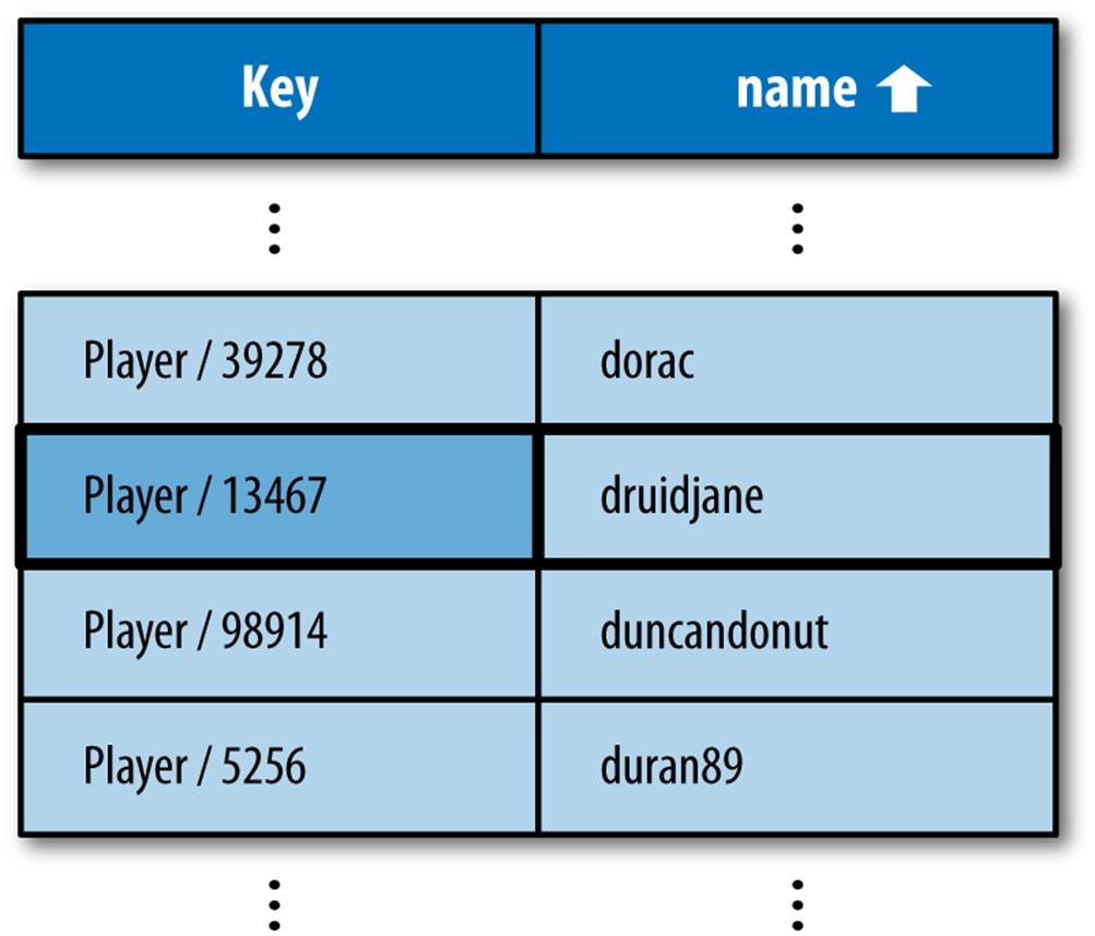
Figure 7-1. An index of Player entity keys and “name” property values, sorted by name in ascending order, with the result for WHERE name = druidjane

To find all entities that meet the conditions of the query, Cloud Datastore finds the first row in the index that matches, then it scans down to the first row that doesn’t match. It returns the entities mentioned on all rows in this range (not counting the nonmatching row), in the order they appear in the index. Because the index is sorted, all results for the query are guaranteed to be on consecutive rows in the table.

Cloud Datastore would use this same index to perform other queries with a similar structure but different values, such as the following query:

SELECT * FROM Player WHERE name = 'duran89'

This query mechanism is fast, even with a very large number of entities. Entities and indexes are distributed across multiple machines, and each machine scans its own index in parallel with the others. Each machine returns results to Cloud Datastore as it scans its own index, and Cloud Datastore delivers the final result set to the app, in order, as if all results were in one large index.

Another reason queries are fast has to do with how the datastore finds the first matching row. Because indexes are sorted, the datastore can use an efficient algorithm to find the first matching row. In the common case, finding the first row takes approximately the same amount of time regardless of the size of the index. In other words, the speed of a query is not affected by the size of the data set.

Cloud Datastore updates all relevant indexes when property values change. In this example, if an application retrieves a Player entity, changes the name, and then saves the entity with a call to the put() method, Cloud Datastore updates the appropriate row in the previous index. It also moves the row if necessary so the ordering of the index is preserved.

Similarly, if the application creates a new Player entity with a name property, or deletes a Player entity with a name property, Cloud Datastore updates the index. In contrast, if the application updates a Player but does not change the name property, or creates or deletes a Player that does not have a name property, Cloud Datastore does not update the name index because no update is needed.

Cloud Datastore maintains two indexes like the previous example for every property name and entity kind, one with the property values sorted in ascending order and one with values in descending order. Cloud Datastore also maintains an index of entities of each kind. These indexes satisfy some simple queries, and Cloud Datastore also uses them internally for bookkeeping purposes.

For other queries, you must tell Cloud Datastore which indexes to prepare. You do this using a configuration file named index.yaml, which gets uploaded along with your application’s code.

It’d be a pain to write this file by hand, but thankfully you don’t have to. While you’re testing your application in the development web server from the SDK, when the app performs a datastore query, the server checks that the configuration file has an appropriate entry for the needed index. If it doesn’t find one, it adds one. As long as the app performs each of its queries at least once during testing, the resulting configuration file will be complete.

The index configuration file must be complete, because when the app is running on App Engine, if the application performs a query for which there is no index, the query returns an error. You can tell the development web server to behave similarly if you want to test for these error conditions. (How to do this depends on which SDK you are using; see “Configuring Indexes”.)

Indexes require a bit of discipline to maintain. Although the development tools can help add index configuration, they cannot know when an index is unused and can be deleted from the file. Extra indexes consume storage space and slow down updates of properties mentioned in the index. And while the version of the app you’re developing may not need a given index, the version of the app still running on App Engine may still need it. The App Engine SDK and the Cloud Console include tools for inspecting and maintaining indexes. We’ll look at these tools in Chapter 20.

Before we discuss index configuration, let’s look more closely at how indexes support queries. We just saw an example where the results for a simple query appear on consecutive rows in a simple index. In fact, this is how most queries work: the results for every query that would use an index appear on consecutive rows in the index. This is both surprisingly powerful in some ways and surprisingly limited in others, and it’s worth understanding why.

Automatic Indexes and Simple Queries

As we mentioned, Cloud Datastore maintains two indexes for every single property of every entity kind, one with values in ascending order and one with values in descending order. Cloud Datastore builds these indexes automatically, regardless of whether they are mentioned in the index configuration file. These automatic indexes satisfy the following kinds of queries using consecutive rows:

§ A simple query for all entities of a given kind, no filters or sort orders

§ One filter on a property using the equality operator (=)

§ Filters using greater-than, greater-than or equal to, less-than, or less-than or equal to operators (>, >=, <, <=) on a single property

§ One sort order, ascending or descending, and no filters, or with filters only on the same property used with the sort order

§ Filters or a sort order on the entity key

§ Kindless queries with or without key filters

Let’s look at each of these in action.

All Entities of a Kind

The simplest datastore query asks for every entity of a given kind, in any order. Stated in GQL, a query for all entities of the kind Player looks like this:

SELECT * FROM Player

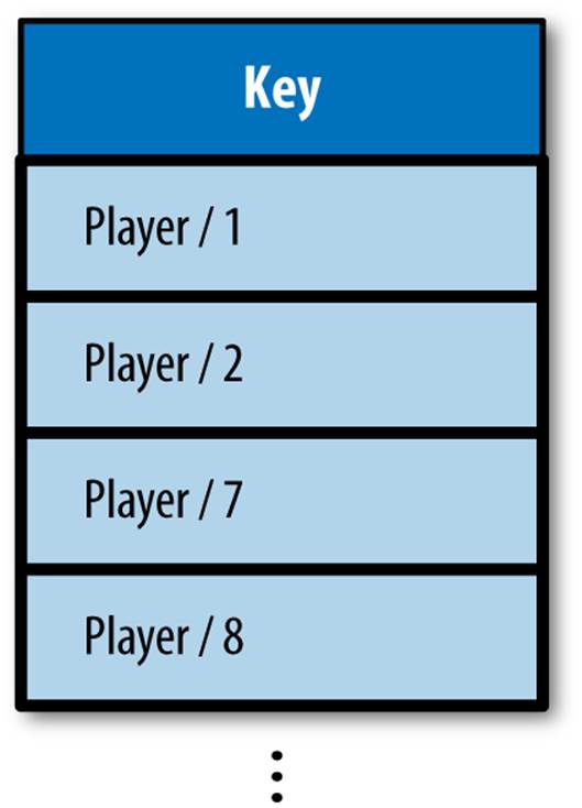
Figure 7-2. An index of all Player entity keys, with results for SELECT * FROM Player

Cloud Datastore maintains an index mapping kinds to entity keys. This index is sorted using a deterministic ordering for entity keys, so this query returns results in “key order.” The kind of an entity cannot be changed after it is created, so this index is updated only when entities are created and deleted.

Because a query can only refer to one kind at a time, you can imagine this index as simply a list of entity keys for each kind. Figure 7-2 illustrates an example of this index.

When the query results are fetched, Cloud Datastore uses the entity keys in the index to find the corresponding entities, and returns the full entities to the application.

One Equality Filter

Consider the following query, which asks for every Player entity with a level property with a value of the integer 10:

SELECT * FROM Player WHERE level = 10

This query uses an index of Player entities with the level property, ascending—one of the automatic indexes. It uses an efficient algorithm to find the first row with a level equal to 10. Then it scans down the index until it finds the first row with a level not equal to 10. The consecutive rows from the first matching to the last matching represent all the Player entities with a level property equal to the integer 10. This is illustrated in Figure 7-3.

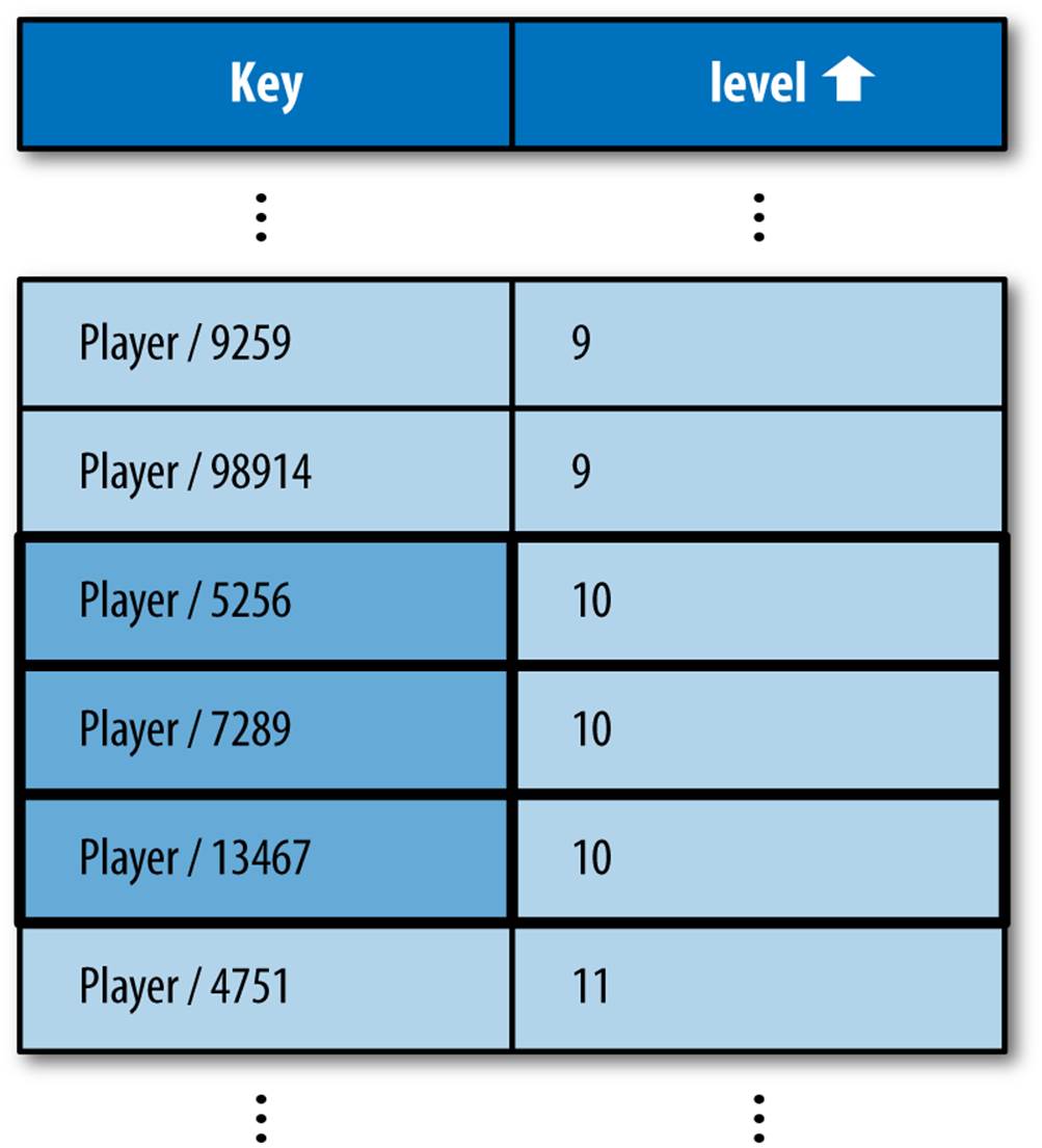
Figure 7-3. An index of the Player entity “level” properties, sorted by level then by key, with results for WHERE level = 10

Greater-Than and Less-Than Filters

The following query asks for every Player entity with a score property whose value is greater than the integer 500:

SELECT * FROM Player WHERE score > 500

This uses an index of Player entities with the score property, ascending, also an automatic index. As with the equality filter, it finds the first row in the index whose score is greater than 500. In the case of greater-than, because the table is sorted by score in ascending order, every row from this point to the bottom of the table is a result for the query. See Figure 7-4.

Similarly, consider a query that asks for every Player with a score less than 1,000:

SELECT * FROM Player WHERE score < 1000

Cloud Datastore uses the same index (score, ascending), and the same strategy: it finds the first row that matches the query, in this case the first row. Then it scans to the next row that doesn’t match the query, the first row whose score is greater than or equal to 1000. The results are represented by everything above that row.

Finally, consider a query for score values between 500 and 1,000:

SELECT * FROM Player WHERE score > 500 AND score < 1000

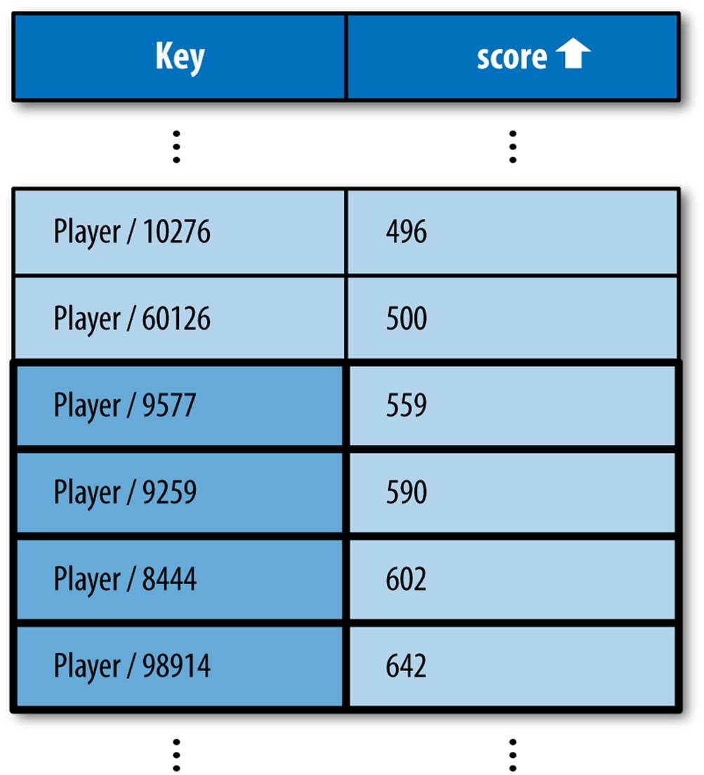
Figure 7-4. An index of the Player entity “score” properties, sorted by score then by key, with results for WHERE score > 500

Once again, the same index and strategy prevail: Cloud Datastore scans from the top down, finding the first matching and next nonmatching rows, returning the entities represented by everything in between. This is shown in Figure 7-5.

If the values used with the filters do not represent a valid range, such as score < 500 AND score > 1000, the query planner notices this and doesn’t bother performing a query, as it knows the query has no results.

One Sort Order

The following query asks for every Player entity, arranged in order by level, from lowest to highest:

SELECT * FROM Player ORDER BY level

As before, this uses an index of Player entities with level properties in ascending order. If both this query and the previous equality query were performed by the application, both queries would use the same index. This query uses the index to determine the order in which to returnPlayer entities, starting at the top of the table and moving down until the application stops fetching results, or until the bottom of the table. Recall that every Player entity with a level property is mentioned in this table. See Figure 7-6.

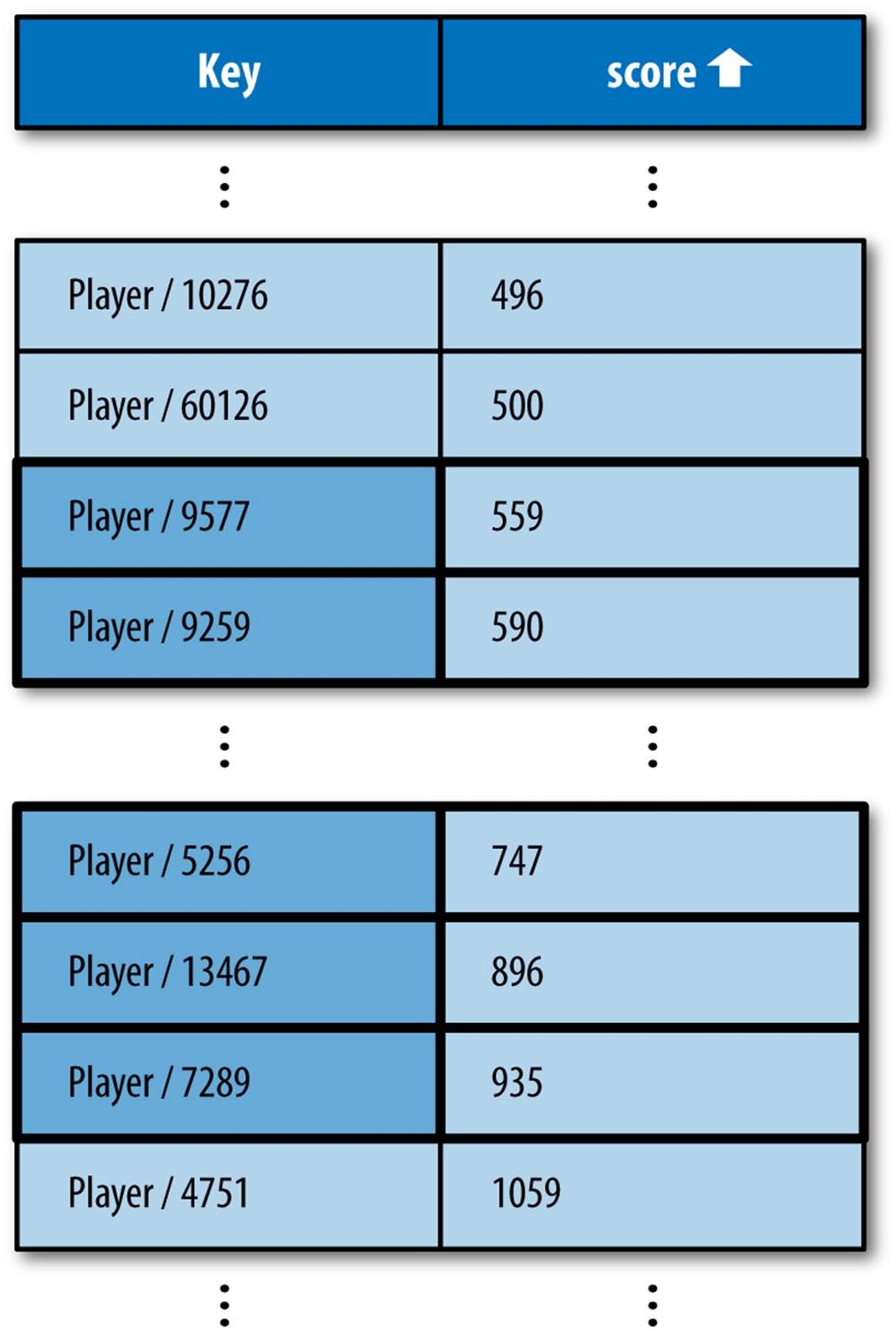
Figure 7-5. An index of the Player entity “score” properties, sorted by score, with results for WHERE score > 500 AND score < 1000

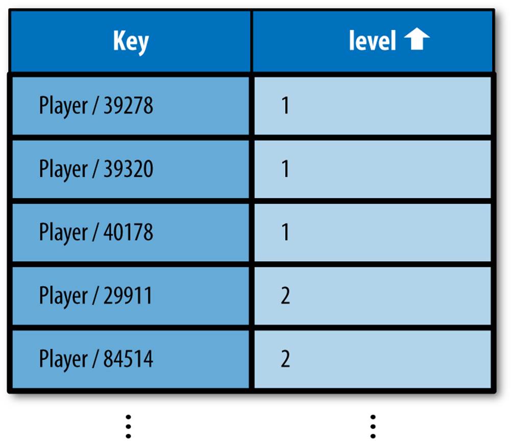
Figure 7-6. An index of the Player entity “level” properties sorted by level in ascending order, with results for ORDER BY level

The following query is similar to the previous one, but asks for the entities arranged by level from highest to lowest:

SELECT * FROM Player ORDER BY level DESC

This query cannot use the same index as before, because the results are in the wrong order. For this query, the results should start at the entity with the highest level, so the query needs an index where this result is in the first row. Cloud Datastore provides an automatic index for single properties in descending order for this purpose. See Figure 7-7.

Figure 7-7. An index of the Player entity “level” properties sorted by level in descending order, with results for ORDER BY level DESC

If a query with a sort order on a single property also includes filters on that property, and no other filters, Cloud Datastore still needs only the one automatic index to fulfill the query. In fact, you may have noticed that for these simple queries, the results are returned sorted by the property in ascending order, regardless of whether the query specifies the sort order explicitly. In these cases, the ascending sort order is redundant.

Queries on Keys

In addition to filters and sort orders on properties, you can also perform queries with filters and sort orders on entity keys. You can refer to an entity’s key in a filter or sort order using the special name __key__.

An equality filter on the key isn’t much use. Only one entity can have a given key, and if the key is known, it’s faster to perform a key.get() than a query. But an inequality filter on the key can be useful for fetching ranges of keys. (If you’re fetching entities in batches, consider using query cursors. See “Query Cursors”.)

Cloud Datastore provides automatic indexes of kinds and keys, sorted by key in ascending order. The query returns the results sorted in key order. This order isn’t useful for display purposes, but it’s deterministic. A query that sorts keys in descending order requires a custom index.

Cloud Datastore uses indexes for filters on keys in the same way as filters on properties, with a minor twist: a query using a key filter in addition to other filters can use an automatic index if a similar query without the key filter could use an automatic index. Automatic indexes for properties already include the keys, so such queries can just use the same indexes. And of course, if the query has no other filters beyond the key filter, it can use the automatic key index.

Kindless Queries

In addition to performing queries on entities of a given kind, the datastore lets you perform a limited set of queries on entities of all kinds. Kindless queries cannot use filters or sort orders on properties. They can, however, use equality and inequality filters on keys (IDs or names).

Kindless queries are mostly useful in combination with ancestors, which we’ll discuss in Chapter 8. They can also be used to get every entity in the datastore. (If you’re querying a large number of entities, you’ll probably want to fetch the results in batches. See “Query Cursors”.)

Using the Query class, you perform a kindless query by omitting the model class argument from the constructor:

q = ndb.Query()

q = q.filter('__key__ >', last_key)

In GQL, you specify a kindless query by omitting the FROM Kind part of the statement:

q = ndb.gql('SELECT * WHERE __key__ > :1', last_key)

The results of a kindless query are returned in key order, ascending. Kindless queries use an automatic index.

NOTE

The datastore maintains statistics about the apps data in a set of datastore entities. When the app performs a kindless query, these statistics entities are included in the results. The kind names for these entities all begin with the characters __Stat_ (two underscores, the word “Stat,” and another underscore). Your app will need to filter these out if they are not desired.

The ndb interface expects there to be an ndb.Model (or ndb.Expando) class defined or imported for each kind of each query result. When using kindless queries, you must define or import all possible kinds. To load classes for the datastore statistics entity kinds, import the ndb.stats module:

from google.appengine.ext.ndb import stats

For more information about datastore statistics, see “Accessing Metadata from the App”.

Custom Indexes and Complex Queries

All queries not covered by the automatic indexes must have corresponding indexes defined in the app’s index configuration file. We’ll refer to these as “custom indexes,” in contrast with “automatic indexes.” Cloud Datastore needs these hints because building every possible index for every combination of property and sort order would take a gargantuan amount of space and time, and an app isn’t likely to need more than a fraction of those possibilities.

In particular, the following queries require custom indexes:

§ A query with multiple sort orders

§ A query with an inequality filter on a property and filters on other properties

§ Projection queries

A query that uses just equality filters on properties does not need a custom index in most cases thanks to a specialized query algorithm for this case, which we’ll look at in a moment. Also, filters on keys do not require custom indexes; they can operate on whatever indexes are used to fulfill the rest of the query.

Let’s examine these queries and the indexes they require. We’ll cover projection queries in “Projection Queries”.

Multiple Sort Orders

The automatic single-property indexes provide enough information for one sort order. When two entities have the same value for the sorted property, the entities appear in the index in adjacent rows, ordered by their entity keys. If you want to order these entities with other criteria, you need an index with more information.

The following query asks for all Player entities, sorted first by the level property in descending order, then, in the case of ties, sorted by the score property in descending order:

SELECT * FROM Player ORDER BY level DESC, score DESC

The index this query needs is straightforward: a table of Player entity keys, level values, and score values, sorted according to the query. This is not one of the indexes provided by the datastore automatically, so it is a custom index, and must be mentioned in the index configuration file. If you performed this query in the development web server, the server would add the following lines to the index.yaml file:

- kind: Player

properties:

- name: level

direction: desc

- name: score

direction: desc

The order the properties appear in the configuration file matters. This is the order in which the rows are sorted: first by level descending, then by score descending.

This configuration creates the index shown in Figure 7-8. The results appear in the table, and are returned for the query in the desired order.

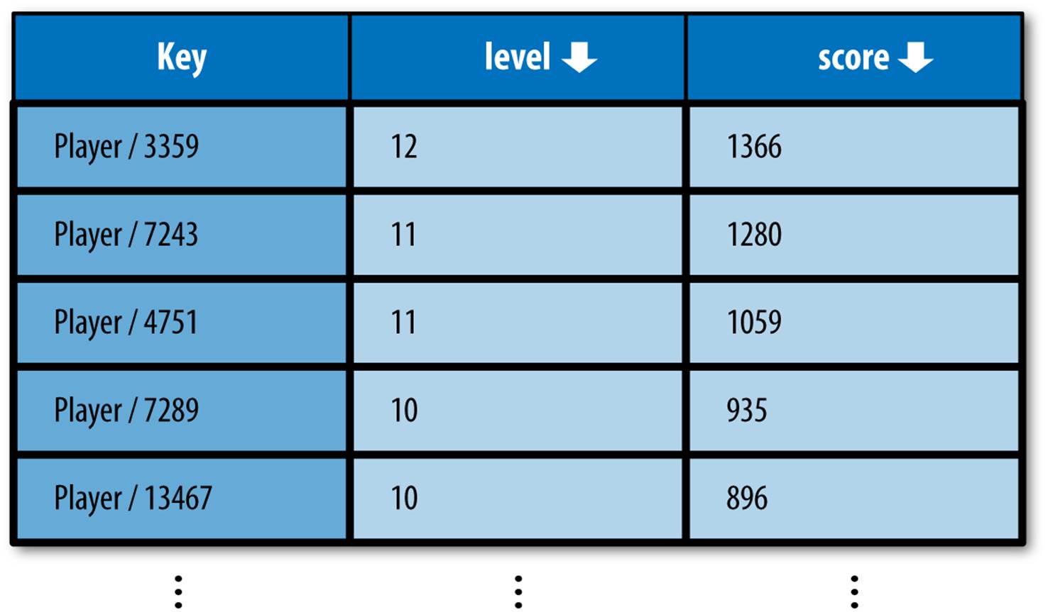
Figure 7-8. An index of the Player entity “level” and “score” properties, sorted by level descending, then score descending, then by key ascending

Filters on Multiple Properties

Consider the following query, which asks for every Player with a level greater than the integer 10 and a charclass of the string 'mage':

SELECT * FROM Player WHERE charclass = 'mage' AND level > 10

To be able to scan to a contiguous set of results meeting both filter criteria, the index must contain columns of values for these properties. The entities must be sorted first by charclass, then by level.

The index configuration for this query would appear as follows in the index.yaml file:

- kind: Player

properties:

- name: charclass

direction: asc

- name: level

direction: asc

This index is illustrated in Figure 7-9.

Figure 7-9. An index of the Player entity “charclass” and “level” properties, sorted by charclass, then level, then key, with results for WHERE charclass = “mage” AND level > 10

The ordering sequence of these properties is important! Remember: the results for the query must all appear on adjacent rows in the index. If the index for this query were sorted first by level then by charclass, it would be possible for valid results to appear on nonadjacent rows.Figure 7-10 demonstrates this problem.

The index ordering requirement for combining inequality and equality filters has several implications that may seem unusual when compared to the query engines of other databases. Heck, they’re downright weird. The first implication, illustrated previously, can be stated generally:

The First Rule of Inequality Filters: If a query uses inequality filters on one property and equality filters on one or more other properties, the index must be ordered first by the properties used in equality filters, then by the property used in the inequality filters.

This rule has a corollary regarding queries with both an inequality filter and sort orders. Consider the following possible query:

SELECT * FROM Player WHERE level > 10 ORDER BY score DESC

Figure 7-10. An index of the Player entity “charclass” and “level” properties, sorted first by level then by charclass, which cannot satisfy WHERE charclass = “mage” AND level > 10 with consecutive rows

What would the index for this query look like? For starters, it would have a column for the level, so it can select the rows that match the filter. It would also have a column for the score, to determine the order of the results. But which column is ordered first?

The First Rule implies that level must be ordered first. But the query requested that the results be returned sorted by score, descending. If the index were sorted by score, then by level, the rows may not be adjacent.

To avoid confusion, Cloud Datastore requires that the correct sort order be stated explicitly in the query:

SELECT * FROM Player WHERE level > 10 ORDER BY level, score DESC

In general:

The Second Rule of Inequality Filters: If a query uses inequality filters on one property and sort orders of one or more other properties, the index must be ordered first by the property used in the inequality filters (in either direction), then by the other desired sort orders. To avoid confusion, the query must state all sort orders explicitly.

There’s one last implication to consider with regard to inequality filters. The following possible query attempts to get all Player entities with a level less than 10 and a score less than 500:

SELECT * FROM Player WHERE level < 10 AND score < 500

Consider an index ordered first by level, then by score, as shown in Figure 7-11.

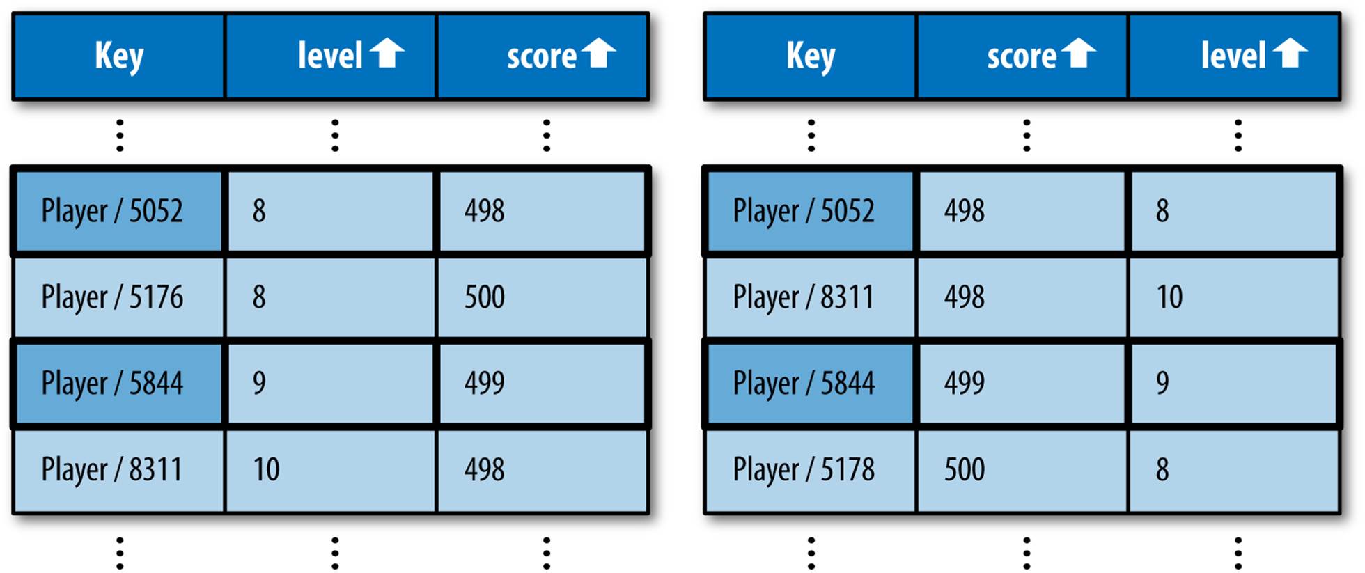
Figure 7-11. Neither possible index of the Player entity “level” and “score” properties can satisfy WHERE level < 10 AND score < 500 with consecutive rows

In fact, there is no possible index that could satisfy this query completely using consecutive rows. This is not a valid datastore query.

The Third Rule of Inequality Filters: A query cannot use inequality filters on more than one property.

A query can use multiple inequality filters on the same property, such as to test for a range of values.

Multiple Equality Filters

For queries using just equality filters, it’s easy to imagine custom indexes that satisfy them. For instance:

SELECT * FROM Player WHERE charclass = 'mage' AND level = 10

A custom index containing these properties, ordered in any sequence and direction, would meet the query’s requirements. But Cloud Datastore has another trick up its sleeve for this kind of query. For queries using just equality filters and no sort orders, instead of scanning a single table of all values, Cloud Datastore can scan the automatic single-property indexes for each property, and return the results as it finds them. Cloud Datastore can perform a “merge join” of the single-property indexes to satisfy this kind of query.

In other words, the datastore doesn’t need a custom index to perform queries using just equality filters and no sort orders. If you add a suitable custom index to your configuration file, the datastore will use it. But a custom index is not required, and the development server’s automatic index configuration feature will not add one if it doesn’t exist.

Let’s consider how the algorithm would perform the following query, using single-property indexes:

SELECT * FROM Kind WHERE a = 1 AND b = 2 AND c = 3

Recall that each of these tables contains a row for each entity with the property set, with fields for the entity’s key and the property’s value. The table is sorted first by the value, then by the key. The algorithm takes advantage of the fact that rows with the same value are consecutive, and within that consecutive block, rows are sorted by key.

To perform the query, the datastore uses the following steps:

1. The datastore checks the a index for the first row with a value of 1. The entity whose key is on this row is a candidate, but not yet a confirmed result.

2. It then checks the b index for the first row whose value is 2 and whose key is greater than or equal to the candidate’s key. Other rows with a value of 2 may appear above this row in the b index, but the datastore knows those are not candidates because the first a scan determined the candidate with the smallest key.

3. If the datastore finds the candidate’s key in the matching region of b, that key is still a candidate, and the datastore proceeds with a similar check in the index for c. If the datastore does not find the candidate in the b index but does find another larger key with a matching value, that key becomes the new candidate, and it proceeds to check for the new candidate in the c index. (It’ll eventually go back to check a with the new candidate before deciding it is a result.) If it finds neither the candidate nor a matching row with a larger key, the query is complete.

4. If a candidate is found to match all criteria in all indexes, the candidate is returned as a result. The datastore starts the search for a new candidate, using the previous candidate’s key as the minimum key.

A key feature of this algorithm is that it finds results in the order in which they are to be returned: key order. The datastore does not need to compile a complete list of possible results for the query—possibly millions of entities—and sort them to determine which results ought to be first. Also, the datastore can stop scanning as soon as it has enough results to fulfill the query, which is always a limited number of entities.

Of course, this query could also use a custom index with all the filter properties in it. If you provide configuration for such an index, the query will use the custom index instead of doing the zigzag join. This can result in a query faster than the zigzag join, at the expense of added time to update the indexed entities.

A zigzag-capable query using equality filters on properties can also use inequality filters on keys without needing a custom index. This is useful for fetching a large number of results in key ranges. (But if you’re fetching batches, cursors might be more effective. See “Query Cursors”.)

Not-Equal and IN Filters

The query API supports two operators we haven’t discussed yet: != (not-equal) and IN. These operators are not actually supported by the datastore itself. Instead, they are implemented by the datastore API as multiple queries in terms of the other operators.

The filter prop != value matches every entity whose property does not equal the value. The datastore API determines the result set by performing two queries: one using prop < value in place of the not-equal filter, and one using prop > value in place of the filter. It returns both sets of results as one result set, which it can do reasonably quickly because the results are already in order.

Because not-equal is actually implemented in terms of the inequality operators, it is subject to the three rules of inequality operators:

§ The query’s index must be ordered by the property used with the not-equal filter before other sort orders.

§ If the query uses other explicit sort orders, the not-equal filter’s property must be explicitly ordered first.

§ And finally, any query using a not-equal filter cannot also use inequality or not-equal filters on other properties.

A not-equal filter will never return an entity that doesn’t have the filtered property. This is true for all filters, but can be especially counterintuitive in the case of not-equal.

To use the not-equal filter in an ndb query expression, simply use Python’s != operator:

q = Player.query().filter(Player.charclass != 'mage')

The filter prop IN (value1, value2, value3) matches every entity whose property equals any of the values. The datastore API implements this as a series of equality queries, one for each value to test. The more values that appear in the list, the longer the full set of queries will take to execute.

With ndb, you specify the IN operator using the IN() method of the property declaration:

q = Player.query().filter(Player.charclass.IN(['mage', 'druid', 'warrior']))

If a single query includes multiple IN filters on multiple properties, the datastore API must perform equality queries for every combination of values in all filters. prop1 IN (value1, value2, value3, value4) AND prop2 IN (value5, value6, value7) is equivalent to 12 queries using equality filters.

The != and IN operators are useful shortcuts. But because they actually perform multiple queries, they take longer to execute than the other operators. It’s worth understanding their performance implications before using them.

Unset and Nonindexed Properties

As you’ve seen, an index contains columns of property values. Typically, an app creates entities of the same kind with the same set of properties: every Player in our game has a name, a character class, a level, and a score. If every entity of a kind has a given property, then an index for that kind and property has a row corresponding to each entity of the kind.

But the datastore neither requires nor enforces a common layout of properties across entities of a kind. It’s quite possible for an entity to not have a property that other entities of the same kind have. For instance, a Player entity might be created without a character class, and go without until the user chooses one.

It is possible to set a property with a null value (None), but a property set to the null value is distinct from the property not being set at all. This is different from a tabular database, which requires a value (possibly null) for every cell in a row.

If an entity does not have a property used in an index, the entity does not appear in the index. Stated conversely, an entity must have every property mentioned in an index to appear in the index. If a Player does not have a charclass property, it does not appear in any index with acharclass column.

If an entity is not mentioned in an index, it cannot be returned as a result for a query that uses the index. Remember that queries use indexes for both filters and sort orders. A query that uses a property for any kind of filter or any sort order can never return an entity that doesn’t have that property. The charclass-less Player can never be a result for a Player query that sorts results by charclass.

In “Strings, Text, and Bytes”, we mentioned that text and blob values are not indexed. Another way of saying this is that, for the purposes of indexes, a property with a text or blob value is treated as if it is unset. If an app performs a query by using a filter or sort order on a property that is always set to a text or blob value, that query will always return no results.

It is sometimes useful to store property values of other types, and exempt them from indexes. This saves space in index tables, and reduces the amount of time it takes to save the entity.

The only way to declare a property as unindexed is with the ndb.Model API. There is currently no other way to set a specific property as unindexed in this API. We’ll look at this feature when we discuss the modeling API in Chapter 9.

If you need an entity to qualify as a result for a query, but it doesn’t make sense in your data model to give the entity every property used in the query, use the null value to represent the “no value” case, and always set it. The Python modeling API makes it easy to ensure that properties always have values.

Sort Orders and Value Types

Cloud Datastore keeps the rows of an index sorted in an order that supports the corresponding query. Each type of property value has its own rules for comparing two values of the same type, and these rules are mostly intuitive: integers are sorted in numeric order, strings in Unicode order, and so forth.

Two entities can have values of different types for the same property, so Cloud Datastore also has rules for comparing such values, although these rules are not so intuitive. Values are ordered first by type, then within their type. For instance, all integers are sorted above all strings.

One effect of this that might be surprising is that all floats are sorted below all integers. The datastore treats floats and integers as separate value types, and so sorts them separately. If your app relies on the correct ordering of numbers, make sure all numbers are stored using the same type of value.

The datastore stores eight distinct types of values, not counting the nonindexed types (text and blob). The datastore supports several additional types by storing them as one of the eight types, then marshaling them between the internal representation and the value your app sees automatically. These additional types are sorted by their internal representation. For instance, a date-time value is actually stored as an integer, and will be sorted among other integer values in an index. (When comparing date-time values, this results in chronological order, which is what you would expect.)

Table 7-2 describes the eight indexable types supported by the datastore. The types are listed in their relative order, from first to last.

Queries and Multivalued Properties

In a typical database, a field in a record stores a single value. A record represents a data object, and each field represents a single, simple aspect of the object. If a data object can have more than one of a particular thing, each of those things is typically represented by a separate record of an appropriate kind, associated with the data object by using the object’s key as a field value. Cloud Datastore supports both of these uses of fields: a property can contain a simple value or the key of another entity.

But Cloud Datastore can do something most other databases can’t: it can store more than one value for a single property. With multivalued properties (MVPs), you can represent a data object with more than one of something without resorting to creating a separate entity for each of those things, if each thing could be represented by a simple value.

One of the most useful features of multivalued properties is how they match an equality filter in a query. The datastore query engine considers a multivalued property equal to a filter value if any of the property’s values is equal to the filter value. This ability to test for membership means MVPs are useful for representing sets.

Multivalued properties maintain the order of values, and can have repeated items. The values can be of any datastore type, and a single property can have values of different types.

MVPs in Code

Consider the following example. The players of our online game can earn trophies for particular accomplishments. The app needs to display a list of all the trophies a player has won, and the app needs to display a list of all the players who have won a particular trophy. The app doesn’t need to maintain any data about the trophies themselves; it’s sufficient to just store the name of the trophy. (This could also be a list of keys for trophy entities.)

One option is to store the list of trophy names as a single delimited string value for each Player entity. This makes it easy to get the list of trophies for a particular player, but impossible to get the list of players for a particular trophy. (A query filter can’t match patterns within string values.)

Another option is to record each trophy win in a separate property named after the trophy. To get the list of players with a trophy, you just query for the existence of the corresponding property. However, getting the list of trophies for a given player would require either coding the names of all the trophies in the display logic, or iterating over all the Player entity’s properties looking for trophy names.

With multivalued properties, we can store each trophy name as a separate value for the trophies property. To access a list of all trophies for a player, we simply access the property of the entity. To get a list of all players with a trophy, we use a query with an equality filter on the property.

In ndb, you can declare that a property is allowed to have multiple values by passing the repeated=True argument to the property declaration:

class Player(ndb.Model):

# ...

trophies = ndb.StringProperty(repeated=True)

The value of the property is a list whose elements are of the appropriate type:

p = ndb.Key(Player, user_id).get()

p.trophies = ['Lava Polo Champion',

'World Building 2008, Bronze',

'Glarcon Fighter, 2nd class']

p.put()

# ...

# List all trophies for a player.

p = ndb.Key(Player, user_id).get()

for trophy inp.trophies:

# ...

# Query all players that have a trophy.

q = Player.gql("WHERE trophies = :1").bind('Lava Polo Champion')

for p inq:

# ...

As with nonrepeated properties, the declaration enforces the type for all values in the list. To declare that a property can contain multiple values of various types, use ndb.GenericProperty(repeated=True). Each member of the list must be of one of the supported datastore types.

With the ndb.Expando base class, you can leave the property undeclared, and simply assign a list value:

class Entity(ndb.Model):

prop = ndb.GenericProperty(repeated=True)

e = Entity()

e.prop = ['value1', 123, users.get_current_user()]

Remember that list is not a datastore type; it is only the mechanism for manipulating multivalued properties. A list cannot contain another list.

Within the datastore, a property must have at least one value, otherwise the property does not exist (the property is unset). The property declaration knows how to translate between the empty list ([]) and the property being unset on an entity. If the property is undeclared (on anndb.Expando), the model class doesn’t know the difference between an empty list value and an unset property, so it behaves as if the property is unset. Take care to handle this case when using ndb.Expando, undeclared properties, and multiple values.

MVPs and Equality Filters

As you’ve seen, when a multivalued property is the subject of an equality filter in a query, the entity matches if any of the property’s values are equal to the filter value:

e1 = Entity()

e1.prop = [3.14, 'a', 'b']

e1.put()

e2 = Entity()

e2.prop = ['a', 1, 6]

e2.put()

# Returns e1 but not e2:

q = Entity.gql('WHERE prop = 3.14')

# Returns e2 but not e1:

q = Entity.gql('WHERE prop = 6')

# Returns both e1 and e2:

q = Entity.gql("WHERE prop = 'a'")

Recall that a query with a single equality filter uses an index that contains the keys of every entity of the given kind with the given property and the property values. If an entity has a single value for the property, the index contains one row that represents the entity and the value. If an entity has multiple values for the property, the index contains one row for each value. The index for this example is shown in Figure 7-13.

This brings us to the first of several odd-looking queries that nonetheless make sense for multivalued properties. Because an equality filter is a membership test, it is possible for multiple equality filters to use the same property with different values and still return a result. An example in GQL:

SELECT * FROM Entity WHERE prop = 'a' AND prop = 'b'

Figure 7-13. An index of two entities with multiple values for the “prop” property, with results for WHERE prop = a

Cloud Datastore uses the “merge join” algorithm, described in “Multiple Equality Filters” for multiple equality filters, to satisfy this query, using the prop single-property index. This query returns the e1 entity because the entity key appears in two places in the index, once for each value requested by the filters.

The way multivalued properties appear in an index gives us another way of thinking about multivalued properties: an entity has one or more properties, each with a name and a single value, and an entity can have multiple properties with the same name. The API represents the values of multiple properties with the same name as a list of values associated with that name.

The datastore does not have a way to query for the exact set of values in a multivalued property. You can use multiple equality filters to test that each of several values belongs to the list, but there is no filter that ensures that those are the only values that belong to the list, or that each value appears only once.

MVPs and Inequality Filters

Just as an equality filter tests that any value of the property is equal to the filter value, an inequality filter tests that any value of the property meets the filter criterion:

e1 = Entity()

e1.prop = [1, 3, 5]

e1.put()

e2 = Entity()

e2.prop = [4, 6, 8]

e2.put()

# Returns e1 but not e2:

q = Entity.gql("WHERE prop < 2")

# Returns e2 but not e1:

q = Entity.gql("WHERE prop > 7")

# Returns both e1 and e2:

q = Entity.gql("WHERE prop > 3")

Figure 7-14 shows the index for this example, with the results of prop > 3 highlighted.

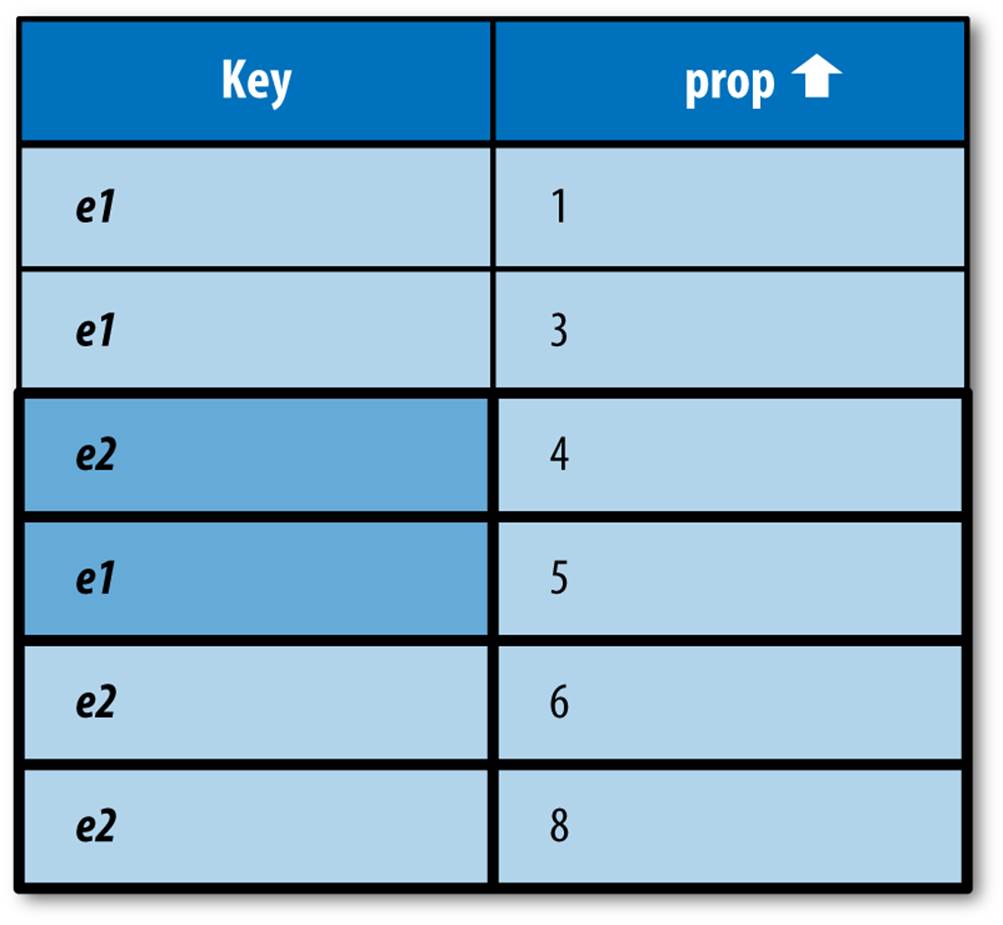
Figure 7-14. An index of two entities with multiple values for the “prop” property, with results for WHERE prop > 3

In the case of an inequality filter, it’s possible for the index scan to match rows for a single entity multiple times. When this happens, the first occurrence of each key in the index determines the order of the results. If the index used for the query sorts the property in ascending order, the first occurrence is the smallest matching value. For descending, it’s the largest. In this example, prop > 3 returns e2 before e1 because 4 appears before 5 in the index.

MVPs and Sort Orders

To summarize things we know about how multivalued properties are indexed:

§ A multivalued property appears in an index with one row per value.

§ All rows in an index are sorted by the values, possibly distributing property values for a single entity across the index.

§ The first occurrence of an entity in an index scan determines its place in the result set for a query.

Together, these facts explain what happens when a query orders its results by a multivalued property. When results are sorted by a multivalued property in ascending order, the smallest value for the property determines its location in the results. When results are sorted in descending order, the largest value for the property determines its location.

This has a counterintuitive—but consistent—consequence:

e1 = Entity()

e1.prop = [1, 3, 5]

e1.put()

e2 = Entity()

e2.prop = [2, 3, 4]

e2.put()

# Returns e1, e2:

q = Entity.gql("ORDER BY prop ASC")

# Also returns e1, e2:

q = Entity.gql("ORDER BY prop DESC")

Because e1 has both the smallest value and the largest value, it appears first in the result set in ascending order and in descending order. See Figure 7-15.

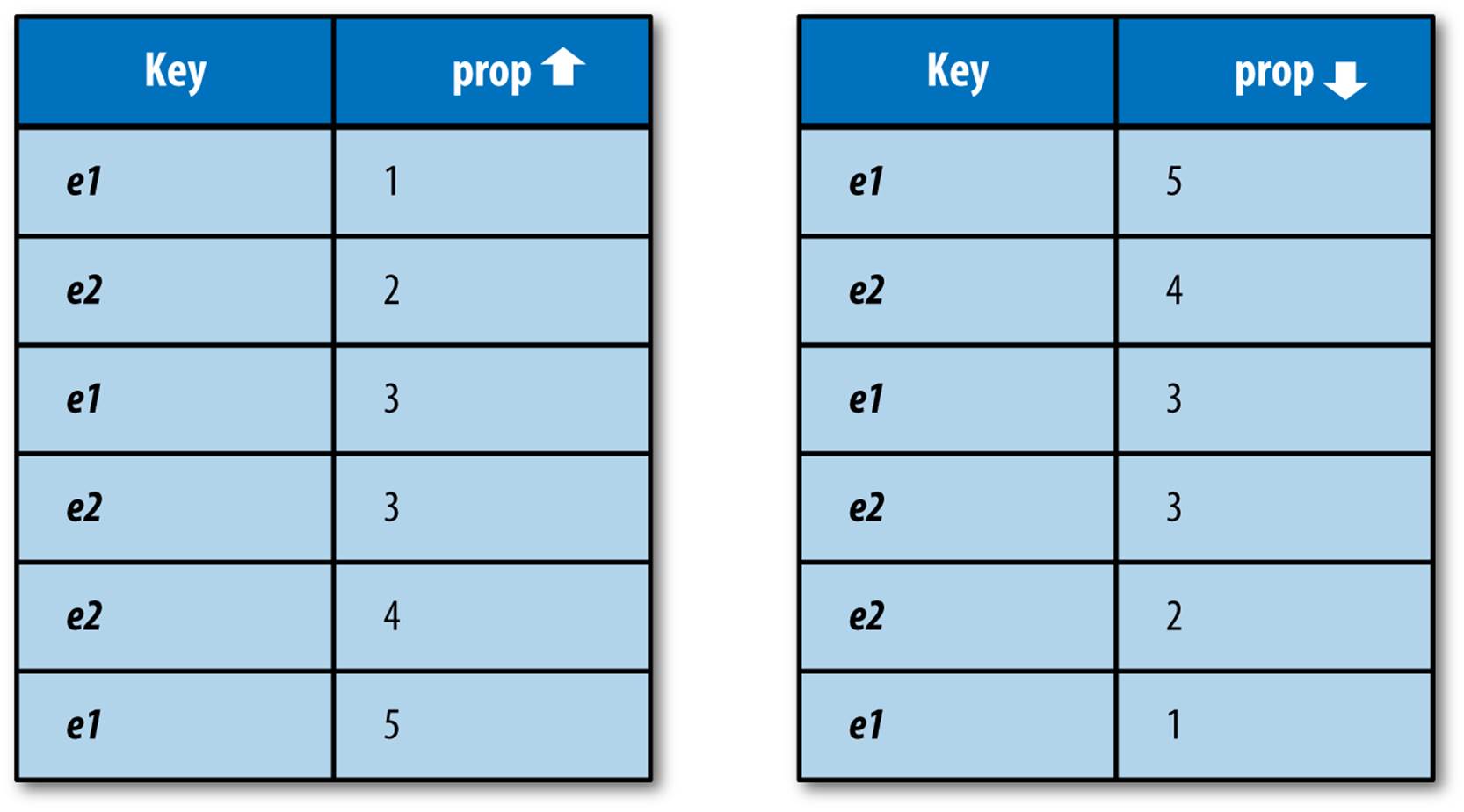
Figure 7-15. Indexes of two entities with multiple values for the “prop” property, one ascending and one descending

MVPS AND THE QUERY PLANNER

The query planner tries to be smart by ignoring aspects of the query that are redundant or contradictory. For instance, a = 3 AND a = 4 would normally return no results, so the query planner catches those cases and doesn’t bother doing work it doesn’t need to do. However, most of these normalization techniques don’t apply to multivalued properties. In this case, the query could be asking, “Does this MVP have a value that is equal to 3 and another value equal to 4?” The datastore remembers which properties are MVPs (even those that end up with one or zero values), and never takes a shortcut that would produce incorrect results.

But there is one exception. A query that has both an equality filter and a sort order on the same property will drop the sort order. If a query asks for a = 3 ORDER BY a DESC and a is a single-value property, the sort order has no effect because all values in the result are identical. For an MVP, however, a = 3 tests for membership, and two MVPs that meet that condition are not necessarily identical.

The datastore drops the sort order in this case anyway. To do otherwise would require too much index data and result in exploding indexes in cases that could otherwise survive. As always, the actual sort order is deterministic, but it won’t be the requested order.

Exploding Indexes

There’s one more thing to know about indexes when considering multivalued properties for your data model.

When an entity has multiple values for a property, each index that includes a column for the property must use multiple rows to represent the entity, one for each possible combination of values. In a single property index on the multivalued property, this is simply one row for each value, two columns each (the entity key and the property value).

In an index of multiple properties where the entity has multiple values for one of the indexed properties and a single value for each of the others, the index includes one row for each value of the multivalued property. Each row has a column for each indexed property, plus the key. The values for the single-value properties are repeated in each row.

Here’s the kicker: if an entity has more than one property with multiple values, and more than one multivalued property appears in an index, the index must contain one row for each combination of values to represent the entity completely.

If you’re not careful, the number of index rows that need to be updated when the entity changes could grow very large. It may be so large that the datastore cannot complete an update of the entity before it reaches its safety limits, and returns an error.

To help prevent “exploding indexes” from causing problems, Cloud Datastore limits the number of property values—that is, the number of rows times the number of columns—a single entity can occupy in an index. The limit is 5,000 property values, high enough for normal use, but low enough to prevent unusual index sizes from inhibiting updates.

If you do include a multivalued property in a custom index, be careful about the possibility of exploding indexes.

Query Cursors

A query often has more results than you want to process in a single action. A message board may have thousands of messages, but it isn’t useful to show a user thousands of messages on one screen. It would be better to show the user a dozen messages at a time, and let the user decide when to look at more, such as by clicking a Next link, or scrolling to the bottom of the display.

A query cursor is like a bookmark in a list of query results. After fetching some results, you can ask the query API for the cursor that represents the spot immediately after the last result you fetched. When you perform the query again at a later time, you can include the cursor value, and the next result fetched will be the one at the spot where the cursor was generated.

Cursors are fast. Unlike with the “offset” fetch parameter, the datastore does not have to scan from the beginning of the results to find the cursor location. The time to fetch results starting from a cursor is proportional to the number of results fetched. This makes cursors ideal for paginated displays of items.

The following is code for a simple paginated display:

import jinja2

import os

import webapp2

from google.appengine.datastore import datastore_query

from google.appengine.ext import ndb

template_env = jinja2.Environment(

loader=jinja2.FileSystemLoader(os.getcwd()))

PAGE_SIZE = 10

class Message(ndb.Model):

create_date = ndb.DateTimeProperty(auto_now_add=True)

# ...

class ResultsPageHandler(webapp2.RequestHandler):

def get(self):

cursor_str = self.request.get('c', None)

cursor = None

if cursor_str:

cursor = datastore_query.Cursor(urlsafe=cursor_str)

query = Message.query().order(-Player.create_date)

results, new_cursor, more = query.fetch_page(

PAGE_SIZE, start_cursor=cursor)

template = template_env.get_template('results.html')

context = {

'results': results,

}

if more:

context['next_cursor'] = new_cursor.urlsafe()

self.response.out.write(template.render(context))

app = webapp2.WSGIApplication([

('/results', ResultsPageHandler),

# ...

],

debug=True)

The results.html template is as follows (note the Next link in particular):

<html><body>

{% if results %}

<p>Messages:</p>

<ul>

{% for result in results %}

<li>{{ result.key.id() }}: {{ result.create_date }}</li>

{% endfor %}

</ul>

{% if next_cursor %}

<p><a href="/results?c={{ next_cursor }}">Next</a></p>

{% endif %}

{% else %}

<p>There are no messages.</p>

{% endif %}

</body></html>

This example displays all of the Message entities in the datastore, in reverse chronological order, in pages of 10 messages per page. If there are more results after the last result displayed, the app shows a Next link back to the request handler with the c parameter set to the cursor pointing to the spot after the last-fetched result. When the user clicks the link, the query is run again, but this time with the cursor value. This causes the next set of results fetched to start where the previous page left off.

The fetch_page() method works just like the fetch() method, but it doesn’t just return the list of results. Instead, it returns a tuple of three elements: the results, a cursor value that represents the end of the fetched results for the query, and a bool that is True if there are more results beyond the cursor. To fetch the next page of results, you call the fetch_page() method on an identical query, passing it the previous cursor value as the start_cursor argument.

The cursor value can be manipulated as a base64-encoded string that is safe to use as a URL query parameter. The cursor returned by fetch_page() is an instance of the Cursor class, from the google.appengine.datastore.datastore_query package. In this example, this value is converted to a URL-safe string via the urlsafe() method, then given to the web page template for use in a link. When the user clicks the link, the request handler sees the encoded value as a query parameter, then makes a new Cursor, passing the URL-safe value as the urlsafe argument to the constructor. The reconstructed Cursor is given to fetch_page().

Note that, like the string form of datastore keys, the base64-encoded value of a cursor can be decoded to reveal the names of kinds and properties, so you may wish to further encrypt or hide the value if these are sensitive.

The fetch_page() method returns the new cursor with the results. You can also use the start_cursor argument with fetch(), iter(), get(), count(), though these methods do not return new cursors. You can also provide an end_cursor argument to any of these methods, after which point the methods will stop returning results. This highlights the “bookmark” nature of cursors: they represent locations in the result set.

TIP

This example shows how to use cursors to set up a Next link in a paginated display. Setting up a Previous link is left as an exercise for the reader. Hint: the cursor used to display the current page, if any, is the one the next page needs for the link.

A cursor is only valid for the query used to generate the cursor value. All query parameters, including kinds, filters, sort orders, and whether or not the query is keys-only, must be identical to the query used to generate the cursor.

A cursor remains valid over time, even if results are added or removed above or below the cursor in the index. A structural change to the indexes used to satisfy the query invalidates cursors for that query. This includes adding or removing fields of a custom index, or switching between built-in indexes and custom indexes for a query. These only occur as a result of you updating your index configuration. Rare internal changes to datastore indexes may also invalidate cursors. Using a cursor that is invalid for a given query (for whatever reason) will raise an exception.

Because a cursor stays valid even after the data changes, you can use cursors to watch for changes in some circumstances. For example, consider a query for entities with creation timestamps, ordered by timestamp. A process traverses the results to the end, and then stores the cursor for the end of the list (with no results after it). When new entities are created with later timestamps, those entities are added to the index after the cursor. Running the query with the cursor pick ups the new results.

NOTE

Conceptually, a cursor is a position in a list of results. Actually, a cursor is a position in the index (or path through multiple indexes) that represents the results for the query. This has a couple of implications.

You can’t use a cursor on a query that uses not-equal (!=) or set membership (IN) queries. These queries are performed by multiple primitive queries behind the scenes, and therefore do not have all results in a single index (or index path).

A query with a cursor may result in a duplicate result if the query operates on a property with multiple values. Recall that an entity with multiple values for a property appears once for each value in the corresponding indexes. When a query gathers results, it ignores repeated results (which are consecutive in the index). Because a cursor represents a point in an index, it is possible for the same entity to appear both before and after the cursor. In this case, the query up to the cursor and the query after the cursor will both contain the entity in their results. It’s a rare edge case—the entity would have to change after the cursor is created—but it’s one to be aware of if you’re using multivalued properties with queries and cursors.

Projection Queries

We’ve described the datastore as an object store. You create an entity with all of its properties. When you fetch an entity by key, the entire entity and all its properties come back. When you want to update a property of an entity, you must fetch the complete entity, make the change to the object locally, then save the entire object back to the datastore.

The types of queries we’ve seen so far reflect this reality as well. You can either fetch entire entities that match query criteria:

SELECT * FROM Kind WHERE ...

Or you can fetch just the keys:

SELECT __key__ FROM Kind WHERE ...

And really, an entity query is just a key query that fetches the entities for those keys. The query criteria drive a scan of an index (or indexes) containing property values and keys, and the keys are returned by the scan.

But sometimes you only need to know one or two properties of an entity, and it’s wasteful to retrieve an entire entity just to get at those properties. For times like these, Cloud Datastore has another trick up its sleeve: projection queries. Projection queries let you request specific properties of entities, instead of full entities, under certain conditions:

SELECT prop1, prop2 FROM Kind WHERE ...

The entity objects that come back have only the requested properties (known as the “projected properties”) and their keys set. Only the requested data is returned by the datastore service to the app.

The idea of projection queries is based on how indexes are used to resolve queries. While a normal query uses indexes of keys and property values to look up keys then fetch the corresponding entities, projection queries take the requested values directly from the indexes themselves.

Naturally, this trick requires that all of the projected properties be present in the index used to fulfill the query. For a projection query requesting only one property, the datastore can use the built-in index. For more than one, you must have a custom index with all of the projected properties in it. As with other complex queries, the development server adds index configuration for each combination of projected properties, kind, and other query criteria.

Projection queries tend to be faster than full queries, for several reasons. Result entities are not fetched in a separate step, as with normal queries. Instead, the result data comes directly from the index. Less data also means less communication with the datastore service. The entire procedure is to find the first row of the custom index and scan to the last row, returning the columns for the projected properties.

Several restrictions fall out of this trick, and they’re fairly intuitive. Only indexed properties can be in a projection. Another way of saying this is, only entities with all the projected properties set to an indexable value can be a result for a projection query. A projection query needs a custom index even if the equivalent full-entity query does not.

There’s another weird behavior we need to note here, and yes, once again it involves multivalued properties. As we saw earlier, if an entity contains multiple values for a property, an index containing that property contains a row for each value (and a row for each combination of values if you’re indexing more than one multivalued property), repeating each of the single-valued properties in the index. Unlike an entity or key query, a projection query makes no attempt to de-duplicate the result list in this case. Instead, a projection on a multivalued property returns a separate result for each row in the index. Each result contains just the values of the properties on that row. Such a query returns one result for each combination of matching property values.

TIP

Each projection of more than one property requires its own custom index. If you have two queries with the same kind and filter structures but different projected properties, the queries require two custom indexes:

SELECT prop1, prop2 FROM Kind ...

SELECT prop1, prop3 FROM Kind ...

In this case, you can save space and time-to-update by using the same projection in both cases, and ignoring the unused properties:

SELECT prop1, prop2, prop3 FROM Kind ...

In ndb, you request a projection query by listing the properties for the projection when you fetch the results, as the projection argument:

q = MyModel.query()

results = q.fetch(10, projection=('prop1', 'prop2'))

You can also use the GQL syntax for projection queries with the ndb.gql() function:

q = ndb.gql('SELECT prop1, prop2 FROM MyModel')

results = q.fetch(10)

The results of a projection query are instances of the model class with only the projected properties set. The model class is aware that the result is from a projection query, and alters its behavior slightly to accommodate. Specifically, it will allow a property modeled as required=True to be unset if it isn’t one of the projected properties. (We’ll cover property modeling in Chapter 9.) Also, it won’t allow the partial instance to be put() back to the datastore, even if you set all of its properties to make it complete.

As a sanity check, the query API will not let you project a property and use it in an equality filter in the same query. It also won’t allow you to project the same property more than once.

As shown, a projection query will return one result for each row in the index it is scanning, which includes one or more rows for each entity that has all of the projected properties. For properties with common values, the results can be a bit repetitive:

class Player(ndb.Model):

# ...

charclass = ndb.StringProperty()

level = ndb.IntegerProperty()

# ...

q = Player.query(projection=('charclass', 'level'))

for result inq:

classlevel = (result.charclass, result.level)

# ...

This might get results like this:

('mage', 1)

('mage', 1)

('mage', 1)

('mage', 2)

('mage', 2)

('mage', 3)

('warrior', 1)

('warrior', 1)

('warrior', 1)

Projection queries have a special feature for when you only want to know which distinct combinations of projected properties exist in the data, eliminating the duplicates. To request this, provide the distinct=True argument:

q = Player.query(projection=('charclass', 'level'),

distinct=True)

In this example, this would reduce the result set to one entry for each distinct combination of the charclass and level values:

('mage', 1)

('mage', 2)

('mage', 3)

('warrior', 1)

Distinct projection queries use only a minor modification to the index scanning algorithm. The rows are scanned in order as before, but a result is only emitted if it differs from the previous row. Only the projected properties are considered: two results are considered equivalent if all of the projected properties are equal between them, even if the nonprojected properties on the corresponding entities are not.

You can do a distinct projection query from GQL using the DISTINCT keyword, like so:

q = ndb.gql('SELECT DISTINCT charclass, level FROM Player')

Configuring Indexes

An application specifies the custom indexes it needs in a configuration file. Each index definition includes the kind, and the names and sort orders of the properties to include. A configuration file can contain zero or more index definitions.

Most of the time, you can leave the maintenance of this file to the development web server. The development server watches the queries the application makes, and if a query needs a custom index and that index is not defined in the configuration file, the server adds appropriate configuration automatically.

The development server will not remove index configuration. If you are sure your app no longer needs an index, you can edit the file manually and remove it. Note that removing index configuration does not automatically delete the index from App Engine. After you upload the new configuration and when you are sure no versions of the app are using the index, you must issue the appcfg vacuum_indexes command. (We’ll cover this in more depth in Chapter 10.)

You can disable the automatic index configuration feature. Doing so causes the development server to behave like App Engine: if a query doesn’t have an index and needs one, the query fails. How to do this is particular to the runtime environment, so we’ll get to that in a moment.

Index configuration is global to all versions of your application. All versions of an app share the same datastore, including indexes. If you deploy a version of the app and the index configuration has changed, Cloud Datastore will use the new index configuration for all versions.

The index configuration file is named index.yaml, and is in the YAML format (similar to app.yaml). It appears in the application root directory.

The structure is a single YAML list named indexes, with one element per index. Each index definition has a kind element (the kind name, a string) and a properties element. If the index supports queries with ancestor filters, it has an ancestor element with a value of yes.

properties is a list, one element per column in the index, where each column has a name and an optional direction that is either asc (ascending order, the default) or desc (descending order). The order of the properties list is significant: the index is sorted by the first column first, then by the second column, and so on.

Here’s an example of an index.yaml file, using indexes from earlier in this chapter:

indexes:

- kind: Player

properties:

- name: charclass

- name: level

direction: desc

- kind: Player

properties:

- name: level

direction: desc

- name: score

direction: desc

By default, the development server adds index configuration to this file as needed. When it does, it does so beneath this line, adding it (and a descriptive comment) if it doesn’t find it:

# AUTOGENERATED

You can move index configuration above this line to take manual control over it. This isn’t strictly necessary, as the development server will never delete index configuration, not even that which was added automatically.

To disable automatic index configuration in the development server, start the server with the --require_indexes command-line option.

1 In ndb, Query objects are immutable, and you use methods to derive new Query objects. This is unlike the old ext.db library, which mutated the Query object directly when methods like filter() were called.