Functional Python Programming (2015)

Chapter 5. Higher-order Functions

A very important feature of the functional programming paradigm is higher-order functions. These are functions that accept functions as arguments or return functions as results. Python offers several of these kinds of functions. We'll look at them and some logical extensions.

As we can see, there are three varieties of higher-order functions, which are as follows:

· Functions that accept a function as one of its arguments

· Functions that return a function

· Functions that accept a function and return a function

Python offers several higher-order functions of the first variety. We'll look at these built-in higher-order functions in this chapter. We'll look at a few of the library modules that offer higher-order functions in later chapters.

The idea of a function that emits functions can seem a bit odd. However, when we look at a Callable class object, we see a function that returns a Callable object. This is one example of a function that creates another function.

Functions that accept functions and create functions include complex Callable classes as well as function decorators. We'll introduce decorators in this chapter, but defer deeper consideration of decorators until Chapter 11, Decorator Design Techniques.

Sometimes we wish that Python had higher-order versions of the collection functions from the previous chapter. In this chapter, we'll show the reduce(extract()) design pattern to perform a reduction on specific fields extracted from a larger tuple. We'll also look at defining our own version of these common collection-processing functions.

In this chapter, we'll look at the following functions:

· max() and min()

· Lambda forms that we can use to simplify using higher-order functions

· map()

· filter()

· iter()

· sorted()

There are a number of higher-order functions in the itertools module. We'll look at this module in Chapter 8, The Itertools Module and Chapter 9, More Itertools Techniques.

Additionally, the functools module provides a general-purpose reduce() function. We'll look at this in Chapter 10, The Functools Module. We'll defer this because it's not as generally applicable as the other higher-order functions in this chapter.

The max() and min() functions are reductions; they create a single value from a collection. The other functions are mappings. They don't reduce the input to a single value.

Note

The max(), min(), and sorted() functions have a default behavior as well as a higher-order function behavior. The function is provided via the key= argument. The map() and filter() functions take the function as the first positional argument.

Using max() and min() to find extrema

The max() and min() functions have a dual life. They are simple functions that apply to collections. They are also higher-order functions. We can see their default behavior as follows:

>>> max(1, 2, 3)

>>> max((1,2,3,4))

Both functions will accept an indefinite number of arguments. The functions are designed to also accept a sequence or an iterable as the only argument and locate the max (or min) of that iterable.

They also do something more sophisticated. Let's say we have our trip data from the examples in Chapter 4, Working with Collections. We have a function that will generate a sequence of tuples that looks as follows:

(((37.54901619777347, -76.33029518659048), (37.840832, -76.273834), 17.7246), ((37.840832, -76.273834), (38.331501, -76.459503), 30.7382), ((38.331501, -76.459503), (38.845501, -76.537331), 31.0756), ((36.843334, -76.298668), (37.549, -76.331169), 42.3962), ((37.549, -76.331169), (38.330166, -76.458504), 47.2866), ((38.330166, -76.458504), (38.976334, -76.473503), 38.8019))

Each tuple has three values: a starting location, an ending location, and a distance. The locations are given in latitude and longitude pairs. The East latitude is positive, so these are points along the US East Coast, about 76° West. The distances are in nautical miles.

We have three ways of getting the maximum and minimum distances from this sequence of values. They are as follows:

· Extract the distance with a generator function. This will give us only the distances, as we've discarded the other two attributes of each leg. This won't work out well if we have any additional processing requirements.

· Use the unwrap(process(wrap())) pattern. This will give us the legs with the longest and shortest distances. From these, we can extract just the distance, if that's all that's needed. The other two will give us the leg that contains the maximum and minimum distances.

· Use the max() and min() functions as higher-order functions.

To provide context, we'll show the first two solutions. The following is a script that builds the trip and then uses the first two approaches to locate the longest and shortest distances traveled:

from ch02_ex3 import float_from_pair, lat_lon_kml, limits, haversine, legs

path= float_from_pair(lat_lon_kml())

trip= tuple((start, end, round(haversine(start, end),4))for start,end in legs(iter(path)))

This section creates the trip object as a tuple based on haversine distances of each leg built from a path read from a KML file.

Once we have the trip object, we can extract distances and compute the maximum and minimum of those distances. The code looks as follows:

long, short = max(dist for start,end,dist in trip), min(dist for start,end,dist in trip)

print(long, short)

We've used a generator function to extract the relevant item from each leg of the trip tuple. We've had to repeat the generator function because each generator expression can be consumed only once.

The following are the results:

129.7748 0.1731

The following is a version with the unwrap(process(wrap())) pattern. We've actually declared functions with the names wrap() and unwrap() to make it clear how this pattern works:

def wrap(leg_iter):

return ((leg[2],leg) for leg in leg_iter)

def unwrap(dist_leg):

distance, leg = dist_leg

return leg

long, short = unwrap(max(wrap(trip))), unwrap(min(wrap(trip)))

print(long, short)

Unlike the previous version, this locates all attributes of the legs with the longest and shortest distances. Rather than simply extracting the distances, we put the distances first in each wrapped tuple. We can then use the default forms of the min() and max() functions to process the two tuples that contain the distance and leg details. After processing, we can strip the first element, leaving just the leg details.

The results look as follows:

((27.154167, -80.195663), (29.195168, -81.002998), 129.7748)

((35.505665, -76.653664), (35.508335, -76.654999), 0.1731)

The final and most important form uses the higher-order function feature of the max() and min() functions. We'll define a helper function first and then use it to reduce the collection of legs to the desired summaries by executing the following code snippet:

def by_dist(leg):

lat, lon, dist= leg

return dist

long, short = max(trip, key=by_dist), min(trip, key=by_dist)

print(long, short)

The by_dist() function picks apart the three items in each leg tuple and returns the distance item. We'll use this with the max() and min() functions.

The max() and min() functions both accept an iterable and a function as arguments. The keyword parameter key= is used by all of Python's higher-order functions to provide a function that will be used to extract the necessary key value.

We can use the following to help conceptualize how the max() function uses the key function:

wrap= ((key(leg),leg) for leg in trip)

return max(wrap)[1]

The max() and min() functions behave as if the given key function is being used to wrap each item in the sequence into a two tuple, process the two tuple, and then decompose the two tuple to return the original value.

Using Python lambda forms

In many cases, the definition of a helper function requires too much code. Often, we can digest the key function to a single expression. It can seem wasteful to have to write both def and return statements to wrap a single expression.

Python offers the lambda form as a way to simplify using higher-order functions. A lambda form allows us to define a small, anonymous function. The function's body is limited to a single expression.

The following is an example of using a simple lambda expression as the key:

long, short = max(trip, key=lambda leg: leg[2]), min(trip, key=lambda leg: leg[2])

print(long, short)

The lambda we've used will be given an item from the sequence; in this case, each leg three tuple will be given to the lambda. The lambda argument variable, leg, is assigned and the expression, leg[2], is evaluated, plucking the distance from the three tuple.

In the rare case that a lambda is never reused, this form is ideal. It's common, however, to need to reuse the lambda objects. Since copy-and-paste is such a bad idea, what's the alternative?

We can always define a function.

We can also assign lambdas to variables, by doing something like this:

start= lambda x: x[0]

end = lambda x: x[1]

dist = lambda x: x[2]

A lambda is a callable object and can be used like a function. The following is an example at the interactive prompt:

>>> leg = ((27.154167, -80.195663), (29.195168, -81.002998), 129.7748)

>>> start= lambda x: x[0]

>>> end = lambda x: x[1]

>>> dist = lambda x: x[2]

>>> dist(leg)

129.7748

Python offers us two ways to assign meaningful names to elements of tuples: namedtuples and a collection of lambdas. Both are equivalent.

To extend this example, we'll look at how we get the latitude or longitude value of the starting or ending point. This is done by defining some additional lambdas.

The following is a continuation of the interactive session:

>>> start(leg)

(27.154167, -80.195663)

>>>

>>> lat = lambda x: x[0]

>>> lon = lambda x: x[1]

>>> lat(start(leg))

27.154167

There's no clear advantage to lambdas over namedtuples. A set of lambdas to extract fields requires more lines of code to define than a namedtuple. On the other hand, we can use a prefix function notation, which might be easier to read in a functional programing context. More importantly, as we'll see in the sorted() example later, the lambdas can be used more effectively than namedtuple attribute names by sorted(), min(), and max().

Lambdas and the lambda calculus

In a book on a purely functional programming language, it would be necessary to explain lambda calculus, and the technique invented by Haskell Curry that we call currying. Python, however, doesn't stick closely to this kind of lambda calculus. Functions are not curried to reduce them to single-argument lambda forms.

We can, using the functools.partial function, implement currying. We'll save this for Chapter 10, The Functools Module.

Using the map() function to apply a function to a collection

A scalar function maps values from a domain to a range. When we look at the math.sqrt() function, as an example, we're looking at a mapping from the float value, x, to another float value, y = sqrt(x) such that . The domain is limited to positive values. The mapping can be done via a calculation or table interpolation.

The map() function expresses a similar concept; it maps one collection to another collection. It assures that a given function is used to map each individual item from the domain collection to the range collection—the ideal way to apply a built-in function to a collection of data.

Our first example involves parsing a block of text to get the sequence of numbers. Let's say we have the following chunk of text:

>>> text= """\

... 2 3 5 7 11 13 17 19 23 29

... 31 37 41 43 47 53 59 61 67 71

... 73 79 83 89 97 101 103 107 109 113

... 127 131 137 139 149 151 157 163 167 173

... 179 181 191 193 197 199 211 223 227 229

... """

We can restructure this text using the following generator function:

>>> data= list(v for line in text.splitlines() for v in line.split())

This will split the text into lines. For each line, it will split the line into space-delimited words and iterate through each of the resulting strings. The results look as follows:

['2', '3', '5', '7', '11', '13', '17', '19', '23', '29', '31', '37', '41', '43', '47', '53', '59', '61', '67', '71', '73', '79', '83', '89', '97', '101', '103', '107', '109', '113', '127', '131', '137', '139', '149', '151', '157', '163', '167', '173', '179', '181', '191', '193', '197', '199', '211', '223', '227', '229']

We still need to apply the int() function to each of the string values. This is where the map() function excels. Take a look at the following code snippet:

>>> list(map(int,data))

[2, 3, 5, 7, 11, 13, 17, 19, 23, 29, 31, 37, 41, 43, 47, 53, 59, 61, 67, 71, 73, 79, 83, 89, 97, 101, 103, 107, 109, 113, 127, 131, 137, 139, 149, 151, 157, 163, 167, 173, 179, 181, 191, 193, 197, 199, 211, 223, 227, 229]

The map() function applied the int() function to each value in the collection. The result is a sequence of numbers instead of a sequence of strings.

The map() function's results are iterable. The map() function can process any type of iterable.

The idea here is that any Python function can be applied to the items of a collection using the map() function. There are a lot of built-in functions that can be used in this map-processing context.

Working with lambda forms and map()

Let's say we want to convert our trip distances from nautical miles to statute miles. We want to multiply each leg's distance by 6076.12/5280, which is 1.150780.

We can do this calculation with the map() function as follows:

map(lambda x: (start(x),end(x),dist(x)*6076.12/5280), trip)

We've defined a lambda that will be applied to each leg in the trip by the map() function. The lambda will use other lambdas to separate the start, end, and distance values from each leg. It will compute a revised distance and assemble a new leg tuple from the start, end, and statute mile distance.

This is precisely like the following generator expression:

((start(x),end(x),dist(x)*6076.12/5280) for x in trip)

We've done the same processing on each item in the generator expression.

The important difference between the map() function and a generator expression is that the map() function tends to be faster than the generator expression. The speedup is in the order of 20 percent less time.

Using map() with multiple sequences

Sometimes, we'll have two collections of data that need to parallel each other. In Chapter 4, Working with Collections, we saw how the zip() function can interleave two sequences to create a sequence of pairs. In many cases, we're really trying to do something like this:

map(function, zip(one_iterable, another_iterable))

We're creating argument tuples from two (or more) parallel iterables and applying a function to the argument tuple. We can also look at it like this:

(function(x,y) for x,y in zip(one_iterable, another_iterable))

Here, we've replaced the map() function with an equivalent generator expression.

We might have the idea of generalizing the whole thing to this:

def star_map(function, *iterables)

return (function(*args) for args in zip(*iterables))

There is a better approach that is already available to us. We don't actually need these techniques. Let's look at a concrete example of the alternate approach.

In Chapter 4, Working with Collections, we looked at trip data that we extracted from an XML file as a series of waypoints. We needed to create legs from this list of waypoints that show the start and end of each leg.

The following is a simplified version that uses the zip() function applied to a special kind of iterable:

>>> waypoints= range(4)

>>> zip(waypoints, waypoints[1:])

<zip object at 0x101a38c20>

>>> list(_)

[(0, 1), (1, 2), (2, 3)]

We've created a sequence of pairs drawn from a single flat list. Each pair will have two adjacent values. The zip() function properly stops when the shorter list is exhausted. This zip( x, x[1:]) pattern only works for materialized sequences and the iterable created by the range() function.

We created pairs so that we can apply the haversine() function to each pair to compute the distance between the two points on the path. The following is how it looks in one sequence of steps:

from ch02_ex3 import lat_lon_kml, float_from_pair, haversine

path= tuple(float_from_pair(lat_lon_kml()))

distances1= map( lambda s_e: (s_e[0], s_e[1], haversine(*s_e)), zip(path, path[1:]))

We've loaded the essential sequence of waypoints into the path variable. This is an ordered sequence of latitude-longitude pairs. As we're going to use the zip(path, path[1:]) design pattern, we must have a materialized sequence and not a simple iterable.

The results of the zip() function will be pairs that have a start and end. We want our output to be a triple with the start, end, and distance. The lambda we're using will decompose the original two tuple and create a new three tuple from the start, end, and distance.

As noted previously, we can simplify this by using a clever feature of the map() function, which is as follows:

distances2= map(lambda s, e: (s, e, haversine(s, e)), path, path[1:])

Note that we've provided a function and two iterables to the map() function. The map() function will take the next item from each iterable and apply those two values as the arguments to the given function. In this case, the given function is a lambda that creates the desired three tuple from the start, end, and distance.

The formal definition for the map() function states that it will do star-map processing with an indefinite number of iterables. It will take items from each iterable to create a tuple of argument values for the given function.

Using the filter() function to pass or reject data

The job of the filter() function is to use and apply a decision function called a predicate to each value in a collection. A decision of True means that the value is passed; otherwise, the value is rejected. The itertools module includes filterfalse() as variations on this theme. Refer to Chapter 8, The Itertools Module to understand the usage of the itertools module's filterfalse() function.

We might apply this to our trip data to create a subset of legs that are over 50 nautical miles long, as follows:

long= list(filter(lambda leg: dist(leg) >= 50, trip)))

The predicate lambda will be True for long legs, which will be passed. Short legs will be rejected. The output is the 14 legs that pass this distance test.

This kind of processing clearly segregates the filter rule (lambda leg: dist(leg) >= 50) from any other processing that creates the trip object or analyzes the long legs.

For another simple example, look at the following code snippet:

>>> filter(lambda x: x%3==0 or x%5==0, range(10))

<filter object at 0x101d5de50>

>>> sum(_)

We've defined a simple lambda to check whether a number is a multiple of three or a multiple of five. We've applied that function to an iterable, range(10). The result is an iterable sequence of numbers that are passed by the decision rule.

The numbers for which the lambda is True are [0, 3, 5, 6, 9], so these values are passed. As the lambda is False for all other numbers, they are rejected.

This can also be done with a generator expression by executing the following code:

>>> list(x for x in range(10) if x%3==0 or x%5==0)

[0, 3, 5, 6, 9]

We can formalize this using the following set comprehension notation:

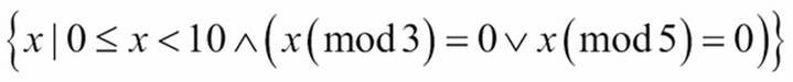
Using the filter() function to pass or reject data

This says that we're building a collection of x values such that x is in range(10) and x%3==0 or x%5==0. There's a very elegant symmetry between the filter() function and formal mathematical set comprehensions.

We often want to use the filter() function with defined functions instead of lambda forms. The following is an example of reusing a predicate defined earlier:

>>> from ch01_ex1 import isprimeg

>>> list(filter(isprimeg, range(100)))

[2, 3, 5, 7, 11, 13, 17, 19, 23, 29, 31, 37, 41, 43, 47, 53, 59, 61, 67, 71, 73, 79, 83, 89, 97]

In this example, we imported a function from another module called isprimeg(). We then applied this function to a collection of values to pass the prime numbers and reject any non-prime numbers from the collection.

This can be a remarkably inefficient way to generate a table of prime numbers. The superficial simplicity of this is the kind of thing lawyers call an attractive nuisance. It looks like it might be fun, but it doesn't scale well at all. A better algorithm is the Sieve of Eratosthenes; this algorithm retains the previously located prime numbers and uses them to prevent a lot of inefficient recalculation.

Using filter() to identify outliers

In the previous chapter, we defined some useful statistical functions to compute mean and standard deviation and normalize a value. We can use these functions to locate outliers in our trip data. What we can do is apply the mean() and stdev() functions to the distance value in each leg of a trip to get the population mean and standard deviation.

We can then use the z() function to compute a normalized value for each leg. If the normalized value is more than 3, the data is extremely far from the mean. If we reject this outliers, we have a more uniform set of data that's less likely to harbor reporting or measurement errors.

The following is how we can tackle this:

from stats import mean, stdev, z

dist_data = list(map(dist, trip))

μ_d = mean(dist_data)

σ_d = stdev(dist_data)

outlier = lambda leg: z(dist(leg),μ_d,σ_d) > 3

print("Outliers", list(filter(outlier, trip)))

We've mapped the distance function to each leg in the trip collection. As we'll do several things with the result, we must materialize a list object. We can't rely on the iterator as the first function will consume it. We can then use this extraction to compute population statistics μ_d and σ_d with the mean and standard deviation.

Given the statistics, we used the outlier lambda to filter our data. If the normalized value is too large, the data is an outlier.

The result of list(filter(outlier, trip)) is a list of two legs that are quite long compared to the rest of the legs in the population. The average distance is about 34 nm, with a standard deviation of 24 nm. No trip can have a normalized distance of less than -1.407.

Note

We're able to decompose a fairly complex problem into a number of independent functions, each one of which can be easily tested in isolation. Our processing is a composition of simpler functions. This can lead to succinct, expressive functional programming.

The iter() function with a sentinel value

The built-in iter() function creates an iterator over a collection object. We can use this to wrap an iterator object around a collection. In many cases, we'll allow the for statement to handle this implicitly. In a few cases, we might want to create an iterator explicitly so that we can separate the head from the tail of a collection. This function can also iterate through the values created by a callable or function until a sentinel value is found. This feature is sometimes used with the read() function of a file to consume rows until some sentinel value is found. In this case, the given function might be some file's readline() method. Providing a callable function to iter() is a bit hard for us because this function must maintain state internally. This hidden state is a feature of an open file, for example, each read() or readline() function advances some internal state to the next character or next line.

Another example of this is the way that a mutable collection object's pop() method makes a stateful change in the object. The following is an example of using the pop() method:

>>> tail= iter([1, 2, 3, None, 4, 5, 6].pop, None)

>>> list(tail)

[6, 5, 4]

The tail variable was set to an iterator over the list [1, 2, 3, None, 4, 5, 6] that will be traversed by the pop() function. The default behavior of pop() is pop(-1), that is, the elements are popped in the reverse order. When the sentinel value is found, the iteratorstops returning values.

This kind of internal state is something we'd like to avoid as much as possible. Consequently, we won't try to contrive a use for this feature.

Using sorted() to put data in order

When we need to produce results in a defined order, Python gives us two choices. We can create a list object and use the list.sort() method to put items in an order. An alternative is to use the sorted() function. This function works with any iterable, but it creates a final list object as part of the sorting operation.

The sorted() function can be used in two ways. It can be simply applied to collections. It can also be used as a higher-order function using the key= argument.

Let's say we have our trip data from the examples in Chapter 4, Working with Collections. We have a function that will generate a sequence of tuples with start, end, and distance for each leg of a trip. The data looks as follows:

We can see the default behavior of the sorted() function using the following interaction:

>>> sorted(dist(x) for x in trip)

[0.1731, 0.1898, 1.4235, 4.3155, ... 86.2095, 115.1751, 129.7748]

We used a generator expression (dist(x) for x in trip) to extract the distances from our trip data. We then sorted this iterable collection of numbers to get the distances from 0.17 nm to 129.77 nm.

If we want to keep the legs and distances together in their original three tuples, we can have the sorted() function apply a key() function to determine how to sort the tuples, as shown in the following code snippet:

>>> sorted(trip, key=dist)

[((35.505665, -76.653664), (35.508335, -76.654999), 0.1731), ((35.028175, -76.682495), (35.031334, -76.682663), 0.1898), ((27.154167, -80.195663), (29.195168, -81.002998), 129.7748)]

We've sorted the trip data, using a dist lambda to extract the distance from each tuple. The dist function is simply as follows:

dist = lambda leg: leg[2]

This shows the power of using simple lambda to decompose a complex tuple into constituent elements.

Writing higher-order functions

We can identify three varieties of higher-order functions; they are as follows:

· Functions that accept a function as one of its arguments.

· Functions that return a function. A Callable class is a common example of this. A function that returns a generator expression can be thought of as a higher-order function.

· Functions that accept and return a function. The functools.partial() function is a common example of this. We'll save this for Chapter 10, The Functools Module. A decorator is different; we'll save this for Chapter 11, Decorator Design Techinques.

We'll expand on these simple patterns using a higher-order function to also transform the structure of the data. We can do several common transformations such as the following:

· Wrap objects to create more complex objects

· Unwrap complex objects into their components

· Flatten a structure

· Structure a flat sequence

A Callable class object is a commonly used example of a function that returns a callable object. We'll look at this as a way to write flexible functions into which configuration parameters can be injected.

We'll also introduce simple decorators in this chapter. We'll defer deeper consideration of decorators until Chapter 11, Decorator Design Techniques.

Writing higher-order mappings and filters

Python's two built-in higher-order functions, map() and filter(), generally handle almost everything we might want to throw at them. It's difficult to optimize them in a general way to achieve higher performance. We'll look at functions of Python 3.4, such as imap(),ifilter(), and ifilterfalse(), in Chapter 8, The Itertools Module.

We have three largely equivalent ways to express a mapping. Assume that we have some function, f(x), and some collection of objects, C. We have three entirely equivalent ways to express a mapping; they are as follows:

· The map() function:

map(f, C)

· The generator expression:

(f(x) for x in C)

· The generator function:

· def mymap(f, C):

· for x in C:

· yield f(x)

mymap(f, C)

Similarly, we have three ways to apply a filter function to a collection, all of which are equivalent:

· The filter() function:

filter(f, C)

· The generator expression:

(x for x in C if f(x))

· The generator function:

· def myfilter(f, C):

· for x in C:

· if f(x):

· yield x

myfilter(f, C)

There are some performance differences; the map() and filter() functions are fastest. More importantly, there are different kinds of extensions that fit these mapping and filtering designs, which are as follows:

· We can create a more sophisticated function, g(x), that is applied to each element, or we can apply a function to the collection, C, prior to processing. This is the most general approach and applies to all three designs. This is where the bulk of our functional design energy is invested.

· We can tweak the for loop. One obvious tweak is to combine mapping and filtering into a single operation by extending the generator expression with an if clause. We can also merge the mymap() and myfilter() functions to combine mapping and filtering.

The profound change we can make is to alter the structure of the data handled by the loop. We have a number of design patterns, including wrapping, unwrapping (or extracting), flattening, and structuring. We've looked at a few of these techniques in previous chapters.

We need to exercise some caution when designing mappings that combine too many transformations in a single function. As far as possible, we want to avoid creating functions that fail to be succinct or expressive of a single idea. As Python doesn't have an optimizing compiler, we might be forced to manually optimize slow applications by combining functions. We need to do this kind of optimization reluctantly, only after profiling a poorly performing program.

Unwrapping data while mapping

When we use a construct such as (f(x) for x, y in C), we've used multiple assignment in the for statement to unwrap a multi-valued tuple and then apply a function. The whole expression is a mapping. This is a common Python optimization to change the structure and apply a function.

We'll use our trip data from Chapter 4, Working with Collections. The following is a concrete example of unwrapping while mapping:

def convert(conversion, trip):

return (conversion(distance) for start, end, distance in trip)

This higher-order function would be supported by conversion functions that we can apply to our raw data as follows:

to_miles = lambda nm: nm*5280/6076.12

to_km = lambda nm: nm*1.852

to_nm = lambda nm: nm

This function would then be used as follows to extract distance and apply a conversion function:

convert(to_miles, trip)

As we're unwrapping, the result will be a sequence of floating-point values. The results are as follows:

[20.397120559090908, 35.37291511060606, ..., 44.652462240151515]

This convert() function is highly specific to our start-end-distance trip data structure, as the for loop decomposes that three tuple.

We can build a more general solution for this kind of unwrapping while mapping a design pattern. It suffers from being a bit more complex. First, we need general-purpose decomposition functions like the following code snippet:

fst= lambda x: x[0]

snd= lambda x: x[1]

sel2= lambda x: x[2]

We'd like to be able to express f(sel2(s_e_d)) for s_e_d in trip. This involves functional composition; we're combining a function like to_miles() and a selector like sel2(). We can express functional composition in Python using yet another lambda, as follows:

to_miles= lambda s_e_d: to_miles(sel2(s_e_d))

This gives us a longer but more general version of unwrapping, as follows:

to_miles(s_e_d) for s_e_d in trip

While this second version is somewhat more general, it doesn't seem wonderfully helpful. When used with particularly complex tuples, however, it can be handy.

What's important to note about our higher-order convert() function is that we're accepting a function as an argument and returning a function as a result. The convert() function is not a generator function; it doesn't yield anything. The result of the convert() function is a generator expression that must be evaluated to accumulate the individual values.

The same design principle works to create hybrid filters instead of mappings. We'd apply the filter in an if clause of the generator expression that was returned.

Of course, we can combine mapping and filtering to create yet more complex functions. It might seem like a good idea to create more complex functions to limit the amount of processing. This isn't always true; a complex function might not beat the performance of a nested use of simple map() and filter() functions. Generally, we only want to create a more complex function if it encapsulates a concept and makes the software easier to understand.

Wrapping additional data while mapping

When we use a construct such as ((f(x), x) for x in C), we've done a wrapping to create a multi-valued tuple while also applying a mapping. This is a common technique to save derived results to create constructs that have the benefits of avoiding recalculation without the liability of complex state-changing objects.

This is part of the example shown in Chapter 4, Working with Collections, to create the trip data from the path of points. The code looks like this:

from ch02_ex3 import float_from_pair, lat_lon_kml, limits, haversine, legs

path= float_from_pair(lat_lon_kml())

trip= tuple((start, end, round(haversine(start, end),4)) for start,end in legs(iter(path)))

We can revise this slightly to create a higher-order function that separates the wrapping from the other functions. We can define a function like this:

def cons_distance(distance, legs_iter):

return ((start, end, round(distance(start,end),4)) for start, end in legs_iter)

This function will decompose each leg into two variables, start and end. These will be used with the given distance() function to compute the distance between the points. The result will build a more complex three tuple that includes the original two legs and also the calculated result.

We can then rewrite our trip assignment to apply the haversine() function to compute distances as follows:

path= float_from_pair(lat_lon_kml())

trip2= tuple(cons_distance(haversine, legs(iter(path))))

We've replaced a generator expression with a higher-order function, cons_distance(). The function not only accepts a function as an argument, but it also returns a generator expression.

A slightly different formulation of this is as follows:

def cons_distance3(distance, legs_iter):

return ( leg+(round(distance(*leg),4),) for leg in legs_iter)

This version makes the construction of a new object built up from an old object a bit clearer. We're iterating through legs of a trip. We're computing the distance along a leg. We're building new structures with the leg and the distance concatenated.

As both of these cons_distance() functions accept a function as an argument, we can use this feature to provide an alternative distance formula. For example, we can use the math.hypot(lat(start)-lat(end), lon(start)-lon(end)) method to compute a less-correct plane distance along each leg.

In Chapter 10, The Functools Module, we'll show how to use the partial() function to set a value for the R parameter of the haversine() function, which changes the units in which the distance is calculated.

Flattening data while mapping

In Chapter 4, Working with Collections, we looked at algorithms that flattened a nested tuple-of-tuples structure into single iterable. Our goal at the time was simply to restructure some data, without doing any real processing. We can create hybrid solutions that combine a function with a flattening operation.

Let's assume that we have a block of text that we want to convert to a flat sequence of numbers. The text looks as follows:

text= """\

2 3 5 7 11 13 17 19 23 29

31 37 41 43 47 53 59 61 67 71

73 79 83 89 97 101 103 107 109 113

127 131 137 139 149 151 157 163 167 173

179 181 191 193 197 199 211 223 227 229

"""

Each line is a block of 10 numbers. We need to unblock the rows to create a flat sequence of numbers.

This is done with a two part generator function as follows:

data= list(v for line in text.splitlines() for v in line.split())

This will split the text into lines and iterate through each line. It will split each line into words and iterate through each word. The output from this is a list of strings, as follows:

To convert the strings to numbers, we must apply a conversion function as well as unwind the blocked structure from its original format, using the following code snippet:

def numbers_from_rows(conversion, text):

return (conversion(v) for line in text.splitlines() for v in line.split())

This function has a conversion argument, which is a function that is applied to each value that will be emitted. The values are created by flattening using the algorithm shown above.

We can use this numbers_from_rows() function in the following kind of expression:

print(list(numbers_from_rows(float, text)))

Here we've used the built-in float() to create a list of floating-point values from the block of text.

We have many alternatives using mixtures of higher-order functions and generator expressions. For example, we might express this as follows:

map(float, v for line in text.splitlines() for v in line.split())

This might be helpful if it helps us understand the overall structure of the algorithm. The principle is called chunking; the details of a function with a meaningful name can be abstracted and we can work with the function in a new context. While we often use higher-order functions, there are times when a generator expression can be more clear.

Structuring data while filtering

The previous three examples combined additional processing with mapping. Combining processing with filtering doesn't seem to be quite as expressive as combining with mapping. We'll look at an example in detail to show that, although it is useful, it doesn't seem to have as compelling a use case as combining mapping and processing.

In Chapter 4, Working with Collections, we looked at structuring algorithms. We can easily combine a filter with the structuring algorithm into a single, complex function. The following is a version of our preferred function to group the output from an iterable:

def group_by_iter(n, iterable):

row= tuple(next(iterable) for i in range(n))

while row:

yield row

row= tuple(next(iterable) for i in range(n))

This will try to assemble a tuple of n items taken from an iterable. If there are any items in the tuple, they are yielded as part of the resulting iterable. In principle, the function then operates recursively on the remaining items from the original iterable. As the recursion is relatively inefficient in Python, we've optimized it into an explicit while loop.

We can use this function as follows:

group_by_iter(7, filter( lambda x: x%3==0 or x%5==0, range(100)))

This will group the results of applying a filter() function to an iterable created by the range() function.

We can merge grouping and filtering into a single function that does both operations in a single function body. The modification to group_by_iter() looks as follows:

def group_filter_iter(n, predicate, iterable):

data = filter(predicate, iterable)

row= tuple(next(data) for i in range(n))

while row:

yield row

row= tuple(next(data) for i in range(n))

This function applies the filter predicate function to the source iterable. As the filter output is itself a non-strict iterable, the data variable isn't computed in advance; the values for data are created as needed. The bulk of this function is identical to the version shown above.

We can slightly simplify the context in which we use this function as follows:

group_filter_iter(7, lambda x: x%3==0 or x%5==0, range(1,100))

Here, we've applied the filter predicate and grouped the results in a single function invocation. In the case of the filter() function, it's rarely a clear advantage to apply the filter in conjunction with other processing. It seems as if a separate, visible filter() function is more helpful than a combined function.

Writing generator functions

Many functions can be expressed neatly as generator expressions. Indeed, we've seen that almost any kind of mapping or filtering can be done as a generator expression. They can also be done with a built-in higher-order function such as map() or filter() or as a generator function. When considering multiple statement generator functions, we need to be cautious that we don't stray from the guiding principles of functional programming: stateless function evaluation.

Using Python for functional programming means walking on a knife edge between purely functional programming and imperative programming. We need to identify and isolate the places where we must resort to imperative Python code because there isn't a purely functional alternative available.

We're obligated to write generator functions when we need statement features of Python. Features like the following aren't available in generator expressions:

· A with context to work with external resources. We'll look at this in Chapter 6, Recursions and Reductions, where we address file parsing.

· A while statement to iterate somewhat more flexibly than a for statement. The example of this is shown previously in the Flattening data while mapping section.

· A break or return statement to implement a search that terminates a loop early.

· The try-except construct to handle exceptions.

· An internal function definition. We've looked at this in several examples in Chapter 1, Introducing Functional Programming and Chapter 2, Introducing Some Functional Features. We'll also revisit it in Chapter 6, Recursions and Reductions.

· A really complex if-elif sequence. Trying to express more than one alternatives via if-else conditional expressions can become complex-looking.

· At the edge of the envelope, we have less-used features of Python such as for-else, while-else, try-else, and try-else-finally. These are all statement-level features that aren't available in generator expressions.

The break statement is most commonly used to end processing of a collection early. We can end processing after the first item that satisfies some criteria. This is a version of the any() function we're looking at to find the existence of a value with a given property. We can also end after processing some larger numbers of items, but not all of them.

Finding a single value can be expressed succinctly as min(some-big-expression) or max(something big). In these cases, we're committed to examining all of the values to assure that we've properly found the minimum or the maximum.

In a few cases, we can stand to have a first(function, collection) function where the first value that is True is sufficient. We'd like the processing to terminate as early as possible, saving needless calculation.

We can define a function as follows:

def first(predicate, collection):

for x in collection:

if predicate(x): return x

We've iterated through the collection, applying the given predicate function. If the predicate is True, we'll return the associated value. If we exhaust the collection, the default value of None will be returned.

We can also download a version of this from PyPi. The first module contains a variation on this idea. For more details visit: https://pypi.python.org/pypi/first.

This can act as a helper when trying to determine whether a number is a prime number or not. The following is a function that tests a number for being prime:

import math

def isprimeh(x):

if x == 2: return True

if x % 2 == 0: return False

factor= first( lambda n: x%n==0, range(3,int(math.sqrt(x)+.5)+1,2))

return factor is None

This function handles a few of the edge cases regarding the number 2 being a prime number and every other even number being composite. Then, it uses the first() function defined above to locate the first factor in the given collection.

When the first() function will return the factor, the actual number doesn't matter. Its existence is all that matters for this particular example. Therefore, the isprimeh() function returns True if no factor was found.

We can do something similar to handle data exceptions. The following is a version of the map() function that also filters bad data:

def map_not_none(function, iterable):

for x in iterable:

try:

yield function(x)

except Exception as e:

pass # print(e)

This function steps through the items in the iterable. It attempts to apply the function to the item; if no exception is raised, this new value is yielded. If an exception is raised, the offending value is silently dropped.

This can be handy when dealing with data that include values that are not applicable or missing. Rather than working out complex filters to exclude these values, we attempt to process them and drop the ones that aren't valid.

We might use the map() function for mapping not-None values as follows:

data = map_not_none(int, some_source)

We'll apply the int() function to each value in some_source. When the some_source parameter is an iterable collection of strings, this can be a handy way to reject strings that don't represent a number.

Building higher-order functions with Callables

We can define higher-order functions as instances of the Callable class. This builds on the idea of writing generator functions; we'll write callables because we need statement features of Python. In addition to using statements, we can also apply a static configuration when creating the higher-order function.

What's important about a Callable class definition is that the class object, created by the class statement, defines essentially a function that emits a function. Commonly, we'll use a callable object to create a composite function that combines two other functions into something relatively complex.

To emphasize this, consider the following class:

from collections.abc import Callable

class NullAware(Callable):

def __init__(self, some_func):

self.some_func= some_func

def __call__(self, arg):

return None if arg is None else self.some_func(arg)

This class creates a function named NullAware() that is a higher-order function that is used to create a new function. When we evaluate the NullAware(math.log) expression, we're creating a new function that can be applied to argument values. The __init__() method will save the given function in the resulting object.

The __call__() method is how the resulting function is evaluated. In this case, the function that was created will gracefully tolerate None values without raising exceptions.

The common approach is to create the new function and save it for future use by assigning it a name as follows:

null_log_scale= NullAware(math.log)

This creates a new function and assigns the name null_log_scale(). We can then use the function in another context. Take a look at the following example:

>>> some_data = [10, 100, None, 50, 60]

>>> scaled = map(null_log_scale, some_data)

>>> list(scaled)

[2.302585092994046, 4.605170185988092, None, 3.912023005428146, 4.0943445622221]

A less common approach is to create and use the emitted function in one expression as follows:

>>> scaled= map(NullAware( math.log ), some_data)

>>> list(scaled)

[2.302585092994046, 4.605170185988092, None, 3.912023005428146, 4.0943445622221]

The evaluation of NullAware( math.log ) created a function. This anonymous function was then used by the map() function to process an iterable, some_data.

This example's __call__() method relies entirely on expression evaluation. It's an elegant and tidy way to define composite functions built up from lower-level component functions. When working with scalar functions, there are a few complex design considerations. When we work with iterable collections, we have to be a bit more careful.

Assuring good functional design

The idea of stateless functional programming requires some care when using Python objects. Objects are typically stateful. Indeed, one can argue that the entire purpose of object-oriented programming is to encapsulate state change into class definition. Because of this, we find ourselves pulled in opposing directions between functional programming and imperative programming when using Python class definitions to process collections.

The benefit of using a Callable to create a composite function gives us slightly simpler syntax when the resulting composite function is used. When we start working with iterable mappings or reductions, we have to be aware of how and why we introduce stateful objects.

We'll return to our sum_filter_f() composite function shown above. Here is a version built from a Callable class definition:

from collections.abc import Callable

class Sum_Filter(Callable):

__slots__ = ["filter", "function"]

def __init__(self, filter, function):

self.filter= filter

self.function= function

def __call__(self, iterable):

return sum(self.function(x) for x in iterable ifself.filter(x))

We've imported the abstract superclass Callable and used this as the basis for our class. We've defined precisely two slots in this object; this puts a few constraints on our ability to use the function as a stateful object. It doesn't prevent all modifications to the resulting object, but it limits us to just two attributes. Attempting to add attributes results in an exception.

The initialization method, __init__(), stows the two function names, filter and function, in the object's instance variables. The __call__() method returns a value based on a generator expression that uses the two internal function definitions. The self.filter()function is used to pass or reject items. The self.function() function is used to transform objects that are passed by the filter() function.

An instance of this class is a function that has two strategy functions built into it. We create an instance as follows:

count_not_none = Sum_Filter(lambda x: x is not None, lambda x: 1)

We've built a function named count_not_none() that counts the non-None values in a sequence. It does this by using a lambda to pass non-None values and a function that uses a constant 1 instead of the actual values present.

Generally, this count_not_none() object will behave like any other Python function. The use is somewhat simpler than our previous example of sum_filter_f().

We can use the count_not_None() function as follows:

N= count_not_none(data)

Instead of using sum_filter_f() funtion:

N= sum_filter_f(valid, count_, data)

The count_not_none() function, based on a Callable, doesn't require quite so many arguments as a conventional function. This makes it superficially simpler to use. However, it can also make it somewhat more obscure because the details of how the function works are in two places in the source code: where the function was created as an instance of the Callable class and where the function was used.

Looking at some of the design patterns

The max(), min(), and sorted() functions have a default behavior without a key= function. They can be customized by providing a function that defines how to compute a key from the available data. For many of our examples, the key() function has been a simple extraction of available data. This isn't a requirement; the key() function can do anything.

Imagine the following method: max(trip, key=random.randint()). Generally, we try not to have have key() functions that do something obscure.

The use of a key= function is a common design pattern. Our functions can easily follow this pattern.

We've also looked at lambda forms that we can use to simplify using higher-order functions. One significant advantage of using lambda forms is that it follows the functional paradigm very closely. When writing more conventional functions, we can create imperative programs that might clutter an otherwise succinct and expressive functional design.

We've looked at several kinds of higher-order functions that work with a collection of values. Throughout the previous chapters, we've hinted around at several different design patterns for higher-order collection and scalar functions. The following is a broad classification:

· Return a Generator. A higher-order function can return a generator expression. We consider the function higher-order because it didn't return scalar values or collections of values. Some of these higher-order functions also accept functions as arguments.

· Act as a Generator. Some function examples use the yield statement to make them first-class generator functions. The value of a generator function is an iterable collection of values that are evaluated lazily. We suggest that a generator function is essentially indistinguishable from a function that returns a generator expression. Both are non-strict. Both can yield a sequence of values. For this reason, we'll also consider generator functions as higher order. Built-in functions such as map() and filter() fall into this category.

· Materialize a Collection. Some functions must return a materialized collection object: list, tuple, set, or mapping. These kinds of functions can be of a higher order if they have a function as part of the arguments. Otherwise, they're ordinary functions that happen to work with collections.

· Reduce a Collection. Some functions work with an iterable (or a collection object) and create a scalar result. The len() and sum() functions are examples of this. We can create higher-order reductions when we accept a function as an argument. We'll return to this in the next chapter.

· Scalar. Some functions act on individual data items. These can be higher-order functions if they accept another function as an argument.

As we design our own software, we can pick and choose among these established design patterns.

Summary

In this chapter, we have seen two reductions that are higher-order functions: max() and min(). We also looked at the two central higher-order functions, map() and filter(). We also looked at sorted().

We also looked at how to use a higher-order function to also transform the structure of data. We can perform several common transformations, including wrapping, unwrapping, flattening, and structure sequences of different kinds.

We looked at three ways to define our own higher-order functions, which are as follows:

· The def statement. Similar to this is a lambda form that we assign to a variable.

· Defining a Callable class as a kind of function that emits composite functions.

· We can also use decorators to emit composite functions. We'll return to this in Chapter 11, Decorator Design Techniques.

In the next chapter, we'll look at the idea of purely functional iteration via recursion. We'll use Pythonic structures to make several common improvements over purely functional techniques. We'll also look at the associated problem of performing reductions from collections to individual values.