Functional Python Programming (2015)
Chapter 6. Recursions and Reductions
In previous chapters, we've looked at several related kinds of processing designs; some of them are as follows:
· Mapping and filtering that create collections from collections
· Reductions that create a scalar value from a collection
The distinction is exemplified by functions such as map() and filter() that accomplish the first kind of collection processing. There are several specialized reduction functions, which include min(), max(), len(), and sum(). There's a general-purpose reduction function, also, functools.reduce().
We'll also consider a collections.Counter() function as a kind of reduction operator. It doesn't produce a single scalar value per se, but it does create a new organization of the data that eliminates some of the original structure. At its heart, it's a kind of count-group-by operation that has more in common with a counting reduction than with a mapping.
In this chapter, we'll look at reduction functions in more detail. From a purely functional perspective, a reduction is defined recursively. For this reason, we'll look at recursion first before we look at reduction algorithms.
Generally, a functional programming language compiler will optimize a recursive function to transform a call in the tail of the function to a loop. This will dramatically improve performance. From a Python perspective, pure recursion is limited, so we must do the tail-call optimization manually. The tail-call optimization technique available in Python is to use an explicit for loop.
We'll look at a number of reduction algorithms including sum(), count(), max(), and min(). We'll also look at the collections.Counter() function and related groupby() reductions. We'll also look at how parsing (and lexical scanning) are proper reductions since they transform sequences of tokens (or sequences of characters) into higher-order collections with more complex properties.
Simple numerical recursions
We can consider all numeric operations to be defined by recursions. For more depth, read about the Peano axioms that define the essential features of numbers. http://en.wikipedia.org/wiki/Peano_axioms is one place to start.
From these axioms, we can see that addition is defined recursively using more primitive notions of the next number, or successor of a number, n, ![]() .
.
To simplify the presentation, we'll assume that we can define a predecessor function,![]() , such that
, such that ![]() , as long as
, as long as ![]()
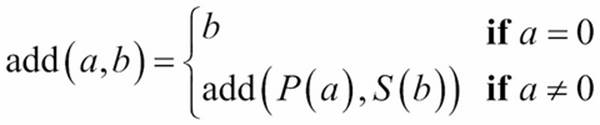
Addition between two natural numbers could be defined recursively as follows:
If we use more common ![]() and
and ![]() instead of
instead of ![]() and
and ![]() , we can see that
, we can see that ![]() .
.
This translates neatly in Python, as shown in the following command snippet:
def add(a,b):
if a == 0: return b
else: return add(a-1, b+1)
We've simply rearranged common mathematical notation into Python. The if clauses are placed to the left instead of the right.
Generally, we don't provide our own functions in Python to do simple addition. We rely on Python's underlying implementation to properly handle arithmetic of various kinds. Our point here is that fundamental scalar arithmetic can be defined recursively.
All of these recursive definitions include at least two cases: the nonrecursive cases where the value of the function is defined directly and recursive cases where the value of the function is computed from a recursive evaluation of the function with different values.
In order to be sure the recursion will terminate, it's important to see how the recursive case computes values that approach the defined nonrecursive case. There are often constraints on the argument values that we've omitted from the functions here. The add()function in the preceding command snippet, for example, can include assert a>= and b>=0 to establish the constraints on the input values.
Without these constraints. a-1 can't be guaranteed to approach the nonrecursive case of a == 0.
In most cases, this is obvious. In a few rare cases, it might be difficult to prove. One example is the Syracuse function. This is one of the pathological cases where termination is unclear.
Implementing tail-call optimization
In the case of some functions, the recursive definition is the one often stated because it is succinct and expressive. One of the most common examples is the factorial() function.
We can see how this is rewritten as a simple recursive function in Python from the following formula:
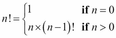
The preceding formula can be executed in Python by using the following commands:
def fact(n):
if n == 0: return 1
else: return n*fact(n-1)
This has the advantage of simplicity. The recursion limits in Python artificially constrain us; we can't do anything larger than about fact(997). The value of 1000! has 2,568 digits and generally exceeds our floating-point capacity; on some systems this is about ![]() Pragmatically, it's common to switch to a log gamma function, which works well with large floating-point values.
Pragmatically, it's common to switch to a log gamma function, which works well with large floating-point values.
This function demonstrates a typical tail recursion. The last expression in the function is a call to the function with a new argument value. An optimizing compiler can replace the function call stack management with a loop that executes very quickly.
Since Python doesn't have an optimizing compiler, we're obliged to look at scalar recursions with an eye toward optimizing them. In this case, the function involves an incremental change from n to n-1. This means that we're generating a sequence of numbers and then doing a reduction to compute their product.
Stepping outside purely functional processing, we can define an imperative facti() calculation as follows:
def facti(n):
if n == 0: return 1
f= 1
for i in range(2,n):
f= f*i
return f
This version of the factorial function will compute values beyond 1000! (2000!, for example, has 5733 digits). It isn't purely functional. We've optimized the tail recursion into a stateful loop depending on the i variable to maintain the state of the computation.
In general, we're obliged to do this in Python because Python can't automatically do the tail-call optimization. There are situations, however, where this kind of optimization isn't actually helpful. We'll look at a few situations.
Leaving recursion in place
In some cases, the recursive definition is actually optimal. Some recursions involve a divide and conquer strategy that minimizes the work from ![]() to
to ![]() . One example of this is the exponentiation by the squaring algorithm. We can state it formally like this:
. One example of this is the exponentiation by the squaring algorithm. We can state it formally like this:
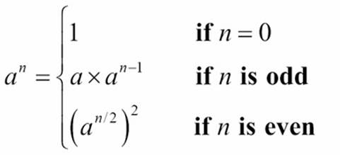
We've broken the process into three cases, easily written in Python as a recursion. Look at the following command snippet:
def fastexp(a, n):
if n == 0: return 1
elif n % 2 == 1: return a*fastexp(a,n-1)
else:
t= fastexp(a,n//2)
return t*t
This function has three cases. The base case, the fastexp(a, 0) method is defined as having a value of 1. The other two cases take two different approaches. For odd numbers, the fastexp() method is defined recursively. The exponent, n, is reduced by 1. A simple tail-recursion optimization would work for this case.
For even numbers, however, the fastexp() recursion uses n/2, chopping the problem into half of its original size. Since the problem size is reduced by a factor of 2, this case results in a significant speed-up of the processing.
We can't trivially reframe this kind of function into a tail-call optimization loop. Since it's already optimal, we don't really need to optimize this further. The recursion limit in Python would impose the constraint of ![]() , a generous upper bound.
, a generous upper bound.
Handling difficult tail-call optimization
We can look at the definition of Fibonacci numbers recursively. Following is one widely used definition for the nth Fibonacci number:
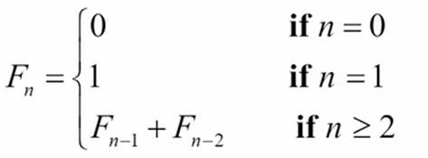
A given Fibonacci number, ![]() , is defined as the sum of the previous two numbers,
, is defined as the sum of the previous two numbers, ![]() . This is an example of multiple recursion: it can't be trivially optimized as a simple tail-recursion. However, if we don't optimize it to a tail-recursion, we'll find it to be too slow to be useful.
. This is an example of multiple recursion: it can't be trivially optimized as a simple tail-recursion. However, if we don't optimize it to a tail-recursion, we'll find it to be too slow to be useful.
The following is a naïve implementation:
def fib(n):
if n == 0: return 0
if n == 1: return 1
return fib(n-1) + fib(n-2)
This suffers from the multiple recursion problem. When computing the fib(n) method, we must compute fib(n-1) and fib(n-2) methods. The computation of fib(n-1) method involves a duplicate calculation of fib(n-2) method. The two recursive uses of the Fibonacci function will duplicate the amount of computation being done.
Because of the left-to-right Python evaluation rules, we can evaluate values up to about fib(1000). However, we have to be patient. Very patient.
Following is an alternative which restates the entire algorithm to use stateful variables instead of a simple recursion:
def fibi(n):
if n == 0: return 0
if n == 1: return 1
f_n2, f_n1 = 1, 1
for i in range(3, n+1):
f_n2, f_n1 = f_n1, f_n2+f_n1
return f_n1
Note
Our stateful version of this function counts up from 0, unlike the recursion, which counts down from the initial value of n. It saves the values of ![]() and
and ![]() that will be used to compute
that will be used to compute ![]() . This version is considerably faster than the recursive version.
. This version is considerably faster than the recursive version.
What's important here is that we couldn't trivially optimize the recursion with an obvious rewrite. In order to replace the recursion with an imperative version, we had to look closely at the algorithm to determine how many stateful intermediate variables were required.
Processing collections via recursion
When working with a collection, we can also define the processing recursively. We can, for example, define the map() function recursively. The formalism looks as follows:
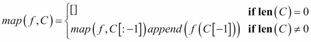
We've defined the mapping of a function to an empty collection as an empty sequence. We've also specified that applying a function to a collection can be defined recursively with a three step expression. First, apply the function to all of the collection except the last element, creating a sequence object. Then apply the function to the last element. Finally, append the last calculation to the previously built sequence.
Following is a purely recursive function version of the older map() function:
def mapr(f, collection):
if len(collection) == 0: return []
return mapr(f, collection[:-1]) + [f(collection[-1])]
The value of the mapr(f,[]) method is defined to be an empty list object. The value of the mapr() function with a non-empty list will apply the function to the last element in the list and append this to the list built recursively from the mapr() function applied to the head of the list.
We have to emphasize that this mapr() function actually creates a list object, similar to the older map() function in Python. The Python 3 map() function is an iterable, and isn't as good an example of tail-call optimization.
While this is an elegant formalism, it still lacks the tail-call optimization required. The tail-call optimization allows us to exceed the recursion depth of 1000 and also performs much more quickly than this naïve recursion.
Tail-call optimization for collections
We have two general ways to handle collections: we can use a higher-order function which returns a generator expression or we can create a function which uses a for loop to process each item in a collection. The two essential patterns are very similar.
Following is a higher-order function that behaves like the built-in map() function:
def mapf(f, C):
return (f(x) for x in C)
We've returned a generator expression which produces the required mapping. This uses an explicit for loop as a kind of tail-call optimization.
Following is a generator function with the same value:
def mapg(f, C):
for x in C:
yield f(x)
This uses a complete for statement for the required optimization.
In both cases, the result is iterable. We must do something following this to materialize a sequence object:
>>> list(mapg(lambda x:2**x, [0, 1, 2, 3, 4]))
[1, 2, 4, 8, 16]
For performance and scalability, this kind of tail-call optimization is essentially required in Python programs. It makes the code less than purely functional. However, the benefit far outweighs the lack of purity. In order to reap the benefits of succinct and expression functional design, it is helpful to treat these less-than-pure functions as if they were proper recursions.
What this means, pragmatically, is that we must avoid cluttering up a collection processing function with additional stateful processing. The central tenets of functional programming are still valid even if some elements of our programs are less than purely functional.
Reductions and folding – from many to one
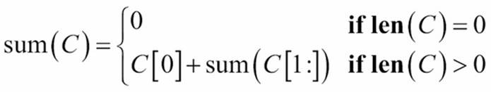
We can consider the sum() function to have the following kind of definition:
We could say that the sum of a collection is 0 for an empty collection. For a non-empty collection the sum is the first element plus the sum of the remaining elements.
Similarly, we can compute the product of a collection of numbers recursively using two cases:

The base case defines the product of an empty sequence as 1. The recursive case defines the product as the first item times the product of the remaining items.
We've effectively folded in × or + operators between each item of the sequence. Further, we've grouped the items so that processing will be done right-to-left. This could be called a fold-right way of reducing a collection to a single value.
In Python, the product function can be defined recursively as follows:
def prodrc(collection):
if len(collection) == 0: return 1
return collection[0] * prodrc(collection[1:])
This is technically correct. It's a trivial rewrite from mathematical notation to Python. However, it is less than optimal because it tends to create a large number of intermediate list objects. It's also limited to only working with explicit collections; it can't work easily with iterable objects.
We can revise this slightly to work with an iterable, which avoids creating any intermediate collection objects. Following is a properly recursive product function which works with an iterable source of data:
def prodri(iterable):
try:
head= next(iterable)
except StopIteration:
return 1
return head*prodri(iterable)
We can't interrogate an iterable with the len() function to see how many elements it has. All we can do is attempt to extract the head of the iterable sequence. If there are no items in the sequence, then any attempt to get the head will raise the StopIterationexception. If there is an item, then we can multiply this item by the product of the remaining items in the sequence. For a demo, we must explicitly create an iterable from a materialized sequence object, using the iter() function. In other contexts, we might have an iterable result that we can use. Following is an example:
>>> prodri(iter([1,2,3,4,5,6,7]))
5040
This recursive definition does not rely on explicit state or other imperative features of Python. While it's more purely functional, it is still limited to working with collections of under 1000 items. Pragmatically, we can use the following kind of imperative structure for reduction functions:
def prodi(iterable):
p= 1
for n in iterable:
p *= n
return p
This lacks the recursion limits. It includes the required tail-call optimization. Further, this will work equally well with either a sequence object or an iterable.
In other functional languages, this is called a foldl operation: the operators are folded into the iterable collection of values from left-to-right. This is unlike the recursive formulations which are generally called foldr operations because the evaluations are done from right-to-left in the collection.
For languages with optimizing compilers and lazy evaluation, the fold-left and fold-right distinction determines how intermediate results are created. This may have profound performance implications, but the distinction might not be obvious. A fold-left, for example, could immediately consume and process the first elements in a sequence. A fold-right, however, might consume the head of the sequence, but not do any processing until the entire sequence was consumed.
Group-by reductions – from many to fewer
A very common operation is a reduction that groups values by some key or indicator. In SQL, this is often called the SELECT GROUP BY operation. The raw data is grouped by some columns value and reductions (sometimes aggregate functions) are applied to other columns. The SQL aggregate functions include SUM, COUNT, MAX, and MIN.
The statistical summary called the mode is a count that's grouped by some independent variable. Python offers us several ways to group data before computing a reduction of the grouped values. We'll start by looking at two ways to get simple counts of grouped data. Then we'll look at ways to compute different summaries of grouped data.
We'll use the trip data that we computed in Chapter 4, Working with Collections. This data started as a sequence of latitude-longitude waypoints. We restructured it to create legs represented by three tuples of start, end, and distance for the leg. The data looks as follows:
(((37.5490162, -76.330295), (37.840832, -76.273834), 17.7246), ((37.840832, -76.273834), (38.331501, -76.459503), 30.7382), ((38.331501, -76.459503), (38.845501, -76.537331), 31.0756), ... ((38.330166, -76.458504), (38.976334, -76.473503), 38.8019))
A common operation that can be approached either as a stateful map or as a materialized, sorted object is computing the mode of a set of data values. When we look at our trip data, the variables are all continuous. To compute a mode, we'll need to quantize the distances covered. This is also called binning: we'll group the data into different bins. Binning is common in data visualization applications, also. In this case, we'll use 5 nautical miles as the size of each bin.
The quantized distances can be produced with a generator expression:
quantized= (5*(dist//5) for start,stop,dist in trip)
This will divide each distance by 5 – discarding any fractions – and then multiply by 5 to compute a number that represents the distance rounded down to the nearest 5 nautical miles.
Building a mapping with Counter
A mapping like the collections.Counter method is a great optimization for doing reductions that create counts (or totals) grouped by some value in the collection. A more typical functional programming solution to grouping data is to sort the original collection, and then use a recursive loop to identify when each group begins. This involves materializing the raw data, performing a  sort, and then doing a reduction to get the sums or counts for each key.
We'll use the following generator to create an simple sequence of distances transformed into bins:
quantized= (5*(dist//5) for start,stop,dist in trip)
We divided each distance by 5 using truncated integer division, and then multiplied by 5 to create a value that's rounded down to the nearest 5 miles.
The following expression creates a mapping from distance to frequency:
from collections import Counter
Counter(quantized)
This is a stateful object, that was created by – technically – imperative object-oriented programming. Since it looks like a function, however, it seems a good fit for a design based on functional programming ideas.
If we print Counter(quantized).most_common() function, we'll see the following results:
[(30.0, 15), (15.0, 9), (35.0, 5), (5.0, 5), (10.0, 5), (20.0, 5), (25.0, 5), (0.0, 4), (40.0, 3), (45.0, 3), (50.0, 3), (60.0, 3), (70.0, 2), (65.0, 1), (80.0, 1), (115.0, 1), (85.0, 1), (55.0, 1), (125.0, 1)]
The most common distance was about 30 nautical miles. The shortest recorded leg was four instances of 0. The longest leg was 125 nautical miles.
Note that your output may vary slightly from this. The results of the most_common() function are in order by frequency; equal-frequency bins may be in any order. These 5 lengths may not always be in the order shown:
(35.0, 5), (5.0, 5), (10.0, 5), (20.0, 5), (25.0, 5)
Building a mapping by sorting
If we want to implement this without using the Counter class, we can use a more functional approach of sorting and grouping. Following is a common algorithm:
def group_sort(trip):
def group(data):
previous, count = None, 0
for d in sorted(data):
if d == previous:
count += 1
elif previous is not None: # and d != previous
yield previous, count
previous, count = d, 1
elif previous is None:
previous, count = d, 1
else:
raise Exception("Bad bad design problem.")
yield previous, count
quantized= (5*(dist//5) for start,stop,dist in trip)
return dict(group(quantized))
The internal group() function steps through the sorted sequence of data items. If a given item has already been seen – it matches the value in previous – then the counter can be incremented. If a given item does not match the previous value and the previous value is not-None, then we've had a change in value; we can emit the previous value and the count, and begin a new accumulation of counts for the new value. The third condition only applies once: if the previous value has never been set, then this is the first value, and we should save it.
The final line of the function creates a dictionary from the grouped items. This dictionary will be similar to a Counter dictionary. The primary difference is that a Counter() function will have a most_common() method function which a default dictionary lacks.
The elif previous is None method case is an irksome overhead. Getting rid of this elif clause (and seeing a slight performance improvement) isn't terribly difficult.
To remove the extra elif clause, we need to use a slightly more elaborate initialization in the internal group() function:
def group(data):
sorted_data= iter(sorted(data))
previous, count = next(sorted_data), 1
for d in sorted_data:
if d == previous:
count += 1
elif previous is not None: # and d != previous
yield previous, count
previous, count = d, 1
else:
raise Exception("Bad bad design problem.")
yield previous, count
This picks the first item out of the set of data to initialize the previous variable. The remaining items are then processed through the loop. This design shows a loose parallel with recursive designs where we initialize the recursion with the first item, and each recursive call provides either a next item or None to indicate that no items are left to process.
We can also do this with itertools.groupby(). We'll look at this function closely in Chapter 8, The Itertools Module.
Grouping or partitioning data by key values
There are no limits to the kinds of reductions we might want to apply to grouped data. We might have data with a number of independent and dependent variables. We can consider partitioning the data by an independent variable and computing summaries like maximum, minimum, average, and standard deviation of the values in each partition.
The essential trick to doing more sophisticated reductions is to collect all of the data values into each group. The Counter() function merely collects counts of identical items. We want to create sequences of the original items based on a key value.
Looked at in a more general way, each 5-mile bin will contain the entire collection of legs of that distance, not merely a count of the legs. We can consider the partitioning as a recursion or as a stateful application of defaultdict(list) object. We'll look at the recursive definition of a groupby() function, since it's easy to design.
Clearly, the groupby(C, key) method for an empty collection, C, is the empty dictionary, dict(). Or, more usefully, the empty defaultdict(list) object.
For a non-empty collection, we need to work with item C[0], the head, and recursively process sequence C[1:], the tail. We can use head, *tail = C command to do this parsing of the collection, as follows:
>>> C= [1,2,3,4,5]
>>> head, *tail= C
>>> head
1
>>> tail
[2, 3, 4, 5]
We need to do the dict[key(head)].append(head) method to include the head element in the resulting dictionary. And then we need to do the groupby(tail,key) method to process the remaining elements.
We can create a function as follows:
def group_by(key, data):
def group_into(key, collection, dictionary):
if len(collection) == 0:
return dictionary
head, *tail= collection
dictionary[key(head)].append(head)
return group_into(key, tail, dictionary)
return group_into(key, data, defaultdict(list))
The interior function handles our essential recursive definition. An empty collection returns the provided dictionary. A non-empty collection is parsed into a head and tail. The head is used to update the dictionary. The tail is then used, recursively, to update the dictionary with all remaining elements.
We can't easily use Python's default values to collapse this into a single function. We cannot use the following command snippet:
def group_by(key, data, dictionary=defaultdict(list)):
If we try this, all uses of the group_by() function share one common defaultdict(list) object. Python builds default values just once. Mutable objects as default values rarely do what we want. Rather than try to include more sophisticated decision-making to handle an immutable default value (like None), we prefer to use a nested function definition. The wrapper() function properly initializes the arguments to the interior function.
We can group the data by distance as follows:
binned_distance = lambda leg: 5*(leg[2]//5)
by_distance= group_by(binned_distance, trip)
We've defined simple, reusable lambda which puts our distances into 5 nm bins. We then grouped the data using the provided lambda.
We can examine the binned data as follows:
import pprint
for distance in sorted(by_distance):
print(distance)
pprint.pprint(by_distance[distance])
Following is what the output looks like:
0.0
[((35.505665, -76.653664), (35.508335, -76.654999), 0.1731), ((35.028175, -76.682495), (35.031334, -76.682663), 0.1898), ((25.4095, -77.910164), (25.425833, -77.832664), 4.3155), ((25.0765, -77.308167), (25.080334, -77.334), 1.4235)]
5.0
[((38.845501, -76.537331), (38.992832, -76.451332), 9.7151), ((34.972332, -76.585167), (35.028175, -76.682495), 5.8441), ((30.717167, -81.552498), (30.766333, -81.471832), 5.103), ((25.471333, -78.408165), (25.504833, -78.232834), 9.7128), ((23.9555, -76.31633), (24.099667, -76.401833), 9.844)] ... 125.0
[((27.154167, -80.195663), (29.195168, -81.002998), 129.7748)]
This can also be written as an iteration as follows:
def partition(key, data):
dictionary= defaultdict(list)
for head in data:
dictionary[key(head)].append(head)
return dictionary
When doing the tail-call optimization, the essential line of the code in the imperative version will match the recursive definition. We've highlighted that line to emphasize that the rewrite is intended to have the same outcome. The rest of the structure represents the tail-call optimization we've adopted as a common way to work around the Python limitations.
Writing more general group-by reductions
Once we have partitioned the raw data, we can compute various kinds of reductions on the data elements in each partition. We might, for example, want the northern-most point for the start of each leg in the distance bins.
We'll introduce some helper functions to decompose the tuple as follows:
start = lambda s, e, d: s
end = lambda s, e, d: e
dist = lambda s, e, d: d
latitude = lambda lat, lon: lat
longitude = lambda lat, lon: lon
Each of these helper functions expects a tuple object to be provided using the * operator to map each element of the tuple to a separate parameter of the lambda. Once the tuple is expanded into the s, e, and p parameters, it's reasonably obvious to return the proper parameter by name. It's much more clear than trying to interpret the tuple_arg[2] method.
Following is how we use these helper functions:
>>> point = ((35.505665, -76.653664), (35.508335, -76.654999), 0.1731)
>>> start(*point)
(35.505665, -76.653664)
>>> end(*point)
(35.508335, -76.654999)
>>> dist(*point)
0.1731
>>> latitude(*start(*point))
35.505665
Our initial point object is a nested three tuple with (0) - a starting position, (1) - the ending position, and (2) - the distance. We extracted various fields using our helper functions.
Given these helpers, we can locate the northern-most starting position for the legs in each bin:
for distance in sorted(by_distance):
print(distance, max(by_distance[distance], key=lambda pt: latitude(*start(*pt))))
The data that we grouped by distance included each leg of the given distance. We supplied all of the legs in each bin to the max() function. The key function we provided to the max() function extracted just the latitude of the starting point of the leg.
This gives us a short list of the northern-most legs of each distance as follows:
0.0 ((35.505665, -76.653664), (35.508335, -76.654999), 0.1731)
5.0 ((38.845501, -76.537331), (38.992832, -76.451332), 9.7151)
10.0 ((36.444168, -76.3265), (36.297501, -76.217834), 10.2537)
...
125.0 ((27.154167, -80.195663), (29.195168, -81.002998), 129.7748)
Writing higher-order reductions
We'll look at an example of a higher-order reduction algorithm here. This will introduce a rather complex topic. The simplest kind of reduction develops a single value from a collection of values. Python has a number of built-in reductions, including any(), all(), max(),min(), sum(), and len().
As we noted in Chapter 4, Working with Collections, we can do a great deal of statistical calculation if we start with a few simple reductions such as the following:
def s0(data):
return sum(1 for x in data) # or len(data)
def s1(data):
return sum(x for x in data) # or sum(data)
def s2(data):
return sum(x*x for x in data)
This allows us to define mean, standard deviation, normalized values, correction, and even least-squares linear regression using a few simple functions.
The last of our simple reductions, s2(), shows how we can apply existing reductions to create higher-order functions. We might change our approach to be more like the following:
def sum_f(function, data):
return sum(function(x) for x in data)
We've added a function that we'll use to transform the data. We'll compute the sum of the transformed values.
Now we can apply this function in three different ways to compute the three essential sums as follows:
N= sum_f(lambda x: 1, data) # x**0
S= sum_f(lambda x: x, data) # x**1
S2= sum_f( lambda x: x*x, data ) # x**2
We've plugged in a small lambda to compute ![]() , which is the count,
, which is the count, ![]() , the sum, and
, the sum, and ![]() , the sum of the squares, which we can use to compute standard deviation.
, the sum of the squares, which we can use to compute standard deviation.
A common extension to this includes a filter to reject raw data which is unknown or unsuitable in some way. We might use the following command to reject bad data:
def sum_filter_f(filter, function, data):
return sum(function(x) for x in data if filter(x))
Execution of the following command snippet allows us to do things like reject None values in a simple way:
count_= lambda x: 1
sum_ = lambda x: x
valid = lambda x: x is not None
N = sum_filter_f(valid, count_, data)
This shows how we can provide two distinct lambda to our sum_filter_f() function. The filter argument is a lambda that rejects None values, we've called it valid to emphasize its meaning. The function argument is a lambda that implements a count or a sum method. We can easily add a lambda to compute a sum of squares.
It's important to note that this function is similar to other examples in that it actually returns a function rather than a value. This is one of the defining characteristics of higher-order functions, and is pleasantly simple to implement in Python.
Writing file parsers
We can often consider a file parser to be a kind of reduction. Many languages have two levels of definition: the lower-level tokens in the language and the higher-level structures built from those tokens. When looking at an XML file, the tags, tag names, and attribute names form this lower-level syntax; the structures which are described by XML form a higher-level syntax.
The lower-level lexical scanning is a kind of reduction that takes individual characters and groups them into tokens. This fits well with Python's generator function design pattern. We can often write functions that look as follows:
Def lexical_scan( some_source ):
for char in some_source:
if some_pattern completed: yield token
else: accumulate token
For our purposes, we'll rely on lower-level file parsers to handle this for us. We'll use the CSV, JSON, and XML packages to manage these details. We'll write higher-level parsers based on these packages.
We'll still rely on a two-level design pattern. A lower-level parser will produce a useful canonical representation of the raw data. It will be an iterator over tuples of text. This is compatible with many kinds of data files. The higher-level parser will produce objects useful for our specific application. These might be tuples of numbers, or namedtuples, or perhaps some other class of immutable Python objects.
We provided one example of a lower-level parser in Chapter 4, Working with Collections. The input was a KML file; KML is an XML representation of geographic information. The essential features of the parser look similar to the following command snippet:
def comma_split(text):
return text.split(",")
def row_iter_kml(file_obj):
ns_map={
"ns0": "http://www.opengis.net/kml/2.2",
"ns1": "http://www.google.com/kml/ext/2.2"}
doc= XML.parse(file_obj)
return (comma_split(coordinates.text)
for coordinates in doc.findall("./ns0:Document/ns0:Folder/ns0:Placemark/ns0:Point/ns0:coordinates", ns_map)
The bulk of the row_iter_kml() function is the XML parsing that allows us to use the doc.findall() function to iterate through the <ns0:coordinates> tags in the document. We've used a function named comma_split() to parse the text of this tag into a three tuple of values.
This is focused on working with the normalized XML structure. The document mostly fits the database designer's definitions of First Normal Form, that is, each attribute is atomic and only a single value. Each row in the XML data had the same columns with data of a consistent type. The data values weren't properly atomic; we had to split the points on a "," to separate longitude, latitude, and altitude into atomic string values.
A large volume of data – xml tags, attributes, and other punctuation – was reduced to a somewhat smaller volume including just floating-point latitude and longitude values. For this reason, we can think of parsers as a kind of reduction.
We'll need a higher-level set of conversions to map the tuples of text into floating-point numbers. Also, we'd like to discard altitude, and reorder longitude and latitude. This will produce the application-specific tuple we need. We can use functions as follows for this conversion:
def pick_lat_lon(lon, lat, alt):
return lat, lon
def float_lat_lon(row_iter):
return (tuple(map(float, pick_lat_lon(*row)))for row in row_iter)
The essential tool is the float_lat_lon() function. This is a higher-order function which returns a generator expression. The generator uses map() function to apply the float() function conversion to the results of pick_lat_lon() class. We've used the *row parameter to assign each member of the row tuple to a different parameter of the pick_lat_lon() function. This function then returns a tuple of the selected items in the required order.
We can use this parser as follows:
with urllib.request.urlopen("file:./Winter%202012-2013.kml") as source:
trip = tuple(float_lat_lon(row_iter_kml(source)))
This will build a tuple-of-tuple representation of each waypoint along the path in the original KML file. It uses a low-level parser to extract rows of text data from the original representation. It uses a high-level parser to transform the text items into more useful tuples of floating-point values. In this case, we have not implemented any validation.
Parsing CSV files
In Chapter 3, Functions, Iterators and Generators, we saw another example where we parsed a CSV file that was not in a normalized form: we had to discard header rows to make it useful. To do this, we used a simple function that extracted the header and returned an iterator over the remaining rows.
The data looks as follows:
Anscombe's quartet
I II III IV
x y x y x y x y
10.0 8.04 10.0 9.14 10.0 7.46 8.0 6.58
8.0 6.95 8.0 8.14 8.0 6.77 8.0 5.76
...
5.0 5.68 5.0 4.74 5.0 5.73 8.0 6.89
The columns are separated by tab characters. Plus there are three rows of headers that we can discard.
Here's another version of that CSV-based parser. We've broken it into three functions. The first, row_iter() function, returns the iterator over the rows in a tab-delimited file. The function looks as follows:
def row_iter_csv(source):
rdr= csv.reader(source, delimiter="\t")
return rdr
This is a simple wrapper around the CSV parsing process. When we look back at the previous parsers for XML and plain text, this was the kind of thing that was missing from those parsers. Producing an iterable over row tuples can be a common feature of parsers for normalized data.
Once we have a row of tuples, we can pass rows that contain usable data and reject rows that contain other metadata, like titles and column names. We'll introduce a helper function that we can use to do some of the parsing, plus a filter() function to validate a row of data.
Following is the conversion:
def float_none(data):
try:
data_f= float(data)
return data_f
except ValueError:
return None
This function handles the conversion of a single string to float values, converting bad data to None value. We can embed this function in a mapping so that we convert all columns of a row to a float or None value. The lambda looks as follows:
float_row = lambda row: list(map(float_none, row))
Following is a row-level validator based on the use of the all() function to assure that all values are float (or none of the values are None):
all_numeric = lambda row: all(row) and len(row) == 8
Following is a higher-order function which combines the row-level conversion and filtering:
def head_filter_map(validator, converter, validator, row_iter):
return filter(all_validator, map(converter, row_iter))
This function gives us a slightly more complete pattern for parsing an input file. The foundation is a lower-level function that iterates over tuples of text. We can then wrap this in functions to convert and validate the converted data. For the cases where files are either in first normal form (all rows are the same) or a simple validator can reject the other rows, this design works out nicely.
All parsing problems aren't quite this simple, however. Some files have important data in header or trailer rows that must be preserved, even though it doesn't match the format of the rest of the file. These non-normalized files will require a more sophisticated parser design.
Parsing plain text files with headers
In Chapter 3, Functions, Iterators, and Generators, the Crayola.GPL file was presented without showing the parser. This file looks as follows:
GIMP Palette
Name: Crayola
Columns: 16
#
239 222 205 Almond
205 149 117 Antique Brass
We can parse a text file using regular expressions. We need to use a filter to read (and parse) header rows. We also want to return an iterable sequence of data rows. This rather complex two-part parsing is based entirely on the two-part – head and tail – file structure.
Following is a low-level parser that handles both head and tail:
def row_iter_gpl(file_obj):
header_pat= re.compile(r"GIMP Palette\nName:\s*(.*?)\nColumns:\s*(.*?)\n#\n", re.M)
def read_head(file_obj):
match= header_pat.match("".join( file_obj.readline() for _ in range(4)))
return (match.group(1), match.group(2)), file_obj
def read_tail(headers, file_obj):
return headers, (next_line.split() for next_line in file_obj)
return read_tail(*read_head(file_obj))
We've defined a regular expression that parses all four lines of the header, and assigned this to the header_pat variable. There are two internal functions for parsing different parts of the file. The read_head() function parses the header lines. It does this by reading four lines and merging them into a single long string. This is then parsed with the regular expression. The results include the two data items from the header plus an iterator ready to process additional lines.
The read_tail() function accepts the output from the read_head() function and parses the iterator over the remaining lines. The parsed information from the header rows forms a two tuple that is given to the read_tail() function along with the iterator over the remaining lines. The remaining lines are merely split on spaces, since that fits the description of the GPL file format.
Note
For more information, visit the following link:
https://code.google.com/p/grafx2/issues/detail?id=518.
Once we've transformed each line of the file into a canonical tuple-of-strings format, we can apply the higher level of parsing to this data. This involves conversion and (if necessary) validation.
Following is a higher-level parser command snippet:
def color_palette(headers, row_iter):
name, columns = headers
colors = tuple(Color(int(r), int(g), int(b), " ".join(name))for r,g,b,*name in row_iter)
return name, columns, colors
This function will work with the output of the lower-level row_iter_gpl() parser: it requires the headers and the iterator. This function will use the multiple assignment to separate the color numbers and the remaining words into four variables, r, g, b, and name. The use of the *name parameter assures that all remaining values will be assigned to names as a tuple. The " ".join(name) method then concatenates the words into a single space-separated string.
Following is how we can use this two-tier parser:
with open("crayola.gpl") as source:
name, columns, colors = color_palette(*row_iter_gpl(source))
print(name, columns, colors)
We've applied the higher-level parser to the results of the lower-level parser. This will return the headers and a tuple built from the sequence of Color objects.
Summary
In this chapter, we've looked at two significant functional programming topics. We've looked at recursions in some detail. Many functional programming language compilers will optimize a recursive function to transform a call in the tail of the function to a loop. In Python, we must do the tail-call optimization manually by using an explicit for loop instead of a purely function recursion.
We've also looked at reduction algorithms including sum(), count(), max(), and min() functions. We looked at the collections.Counter() function and related groupby() reductions.
We've also looked at how parsing (and lexical scanning) are similar to reductions since they transform sequences of tokens (or sequences of characters) into higher-order collections with more complex properties. We've examined a design pattern that decomposes parsing into a lower level that tries to produce tuples of raw strings and a higher level that creates more useful application objects.
In the next chapter, we'll look at some techniques appropriate to working with namedtuples and other immutable data structures. We'll look at techniques that make stateful objects unnecessary. While stateful objects aren't purely functional, the idea of a class hierarchy can be used to package related method function definitions.
All materials on the site are licensed Creative Commons Attribution-Sharealike 3.0 Unported CC BY-SA 3.0 & GNU Free Documentation License (GFDL)
If you are the copyright holder of any material contained on our site and intend to remove it, please contact our site administrator for approval.
© 2016-2026 All site design rights belong to S.Y.A.