Functional Python Programming (2015)

Chapter 7. Additional Tuple Techniques

Many of the examples we've looked at have either been scalar functions, or relatively simple structures built from small tuples. We can often exploit Python's immutable namedtuple as a way to build complex data structures. We'll look at how we use and how we create namedtuples. We'll also look at ways that immutable namedtuples can be used instead of stateful object classes.

One of the beneficial features of object-oriented programming is the ability to create complex data structures incrementally. In some respects, an object is simply a cache for results of functions; this will often fit well with functional design patterns. In other cases, the object paradigm provides for property methods that include sophisticated calculations. This is an even better fit for functional design ideas.

In some cases, however, object class definitions are used statefully to create complex objects. We'll look at a number of alternatives that provide similar features without the complexities of stateful objects. We can identify stateful class definitions and then include meta-properties for valid or required ordering of method function calls. Statements such as If X.p() is called before X.q(), the results are undefined are outside the formalism of the language and are meta-properties of a class. Sometimes, stateful classes include the overhead of explicit assertions and error checking to assure that methods are used in the proper order. If we avoid stateful classes, we eliminate these kinds of overheads.

We'll also look at some techniques to write generic functions outside any polymorphic class definition. Clearly, we can rely on Callable classes to create a polymorphic class hierarchy. In some cases, this might be a needless overhead in a functional design.

Using an immutable namedtuple as a record

In Chapter 3, Functions, Iterators, and Generators, we showed two common techniques to work with tuples. We've also hinted at a third way to handle complex structures. We can do any of the following, depending on the circumstances:

· Use lambdas (or functions) to select a named item using the index

· Use lambdas (or functions) with *parameter to select an item by parameter name, which maps to an index

· Use namedtuples to select an item by attribute name or index

Our trip data, introduced in Chapter 4, Working with Collections, has a rather complex structure. The data started as an ordinary time series of position reports. To compute the distances covered, we transposed the data into a sequence of legs with a start position, end position, and distance as a nested three-tuple.

Each item in the sequence of legs looks as follows as a three-tuple:

first_leg= ((37.54901619777347, -76.33029518659048), (37.840832, -76.273834), 17.7246)

This is a short trip between two points on the Chesapeake Bay.

A nested tuple of tuples can be rather difficult to read; for example, expressions such as first_leg[0][0] aren't very informative.

Let's look at the three alternatives for selected values out of a tuple. The first technique involves defining some simple selection functions that can pick items from a tuple by index position:

start= lambda leg: leg[0]

end= lambda leg: leg[1]

distance= lambda leg: leg[2]

latitude= lambda pt: pt[0]

longitude= lambda pt: pt[1]

With these definitions, we can use latitude(start(first_leg)) to refer to a specific piece of data.

These definitions don't provide much guidance on the data types involved. We can use a simple naming convention to make this a bit more clear. The following are some examples of selection functions that use a suffix:

start_point = lambda leg: leg[0]

distance_nm= lambda leg: leg[2]

latitude_value= lambda point: point[0]

When used judiciously, this can be helpful. It can also degenerate into an elaborately complex Hungarian notation as a prefix (or suffix) of each variable.

The second technique uses the *parameter notation to conceal some details of the index positions. The following are some selection functions that use the * notation:

start= lambda start, end, distance: start

end= lambda start, end, distance: end

distance= lambda start, end, distance: distance

latitude= lambda lat, lon: lat

longitude= lambda lat, lon: lon

With these definitions, we can use latitude(*start(*first_leg)) to refer to a specific piece of data. This has the advantage of clarity. It can look a little odd to see the * operator in front of the tuple arguments to these selection functions.

The third technique is the namedtuple function. In this case, we have nested namedtuple functions such as the following:

Leg = namedtuple("Leg", ("start", "end", "distance"))

Point = namedtuple("Point", ("latitude", "longitude"))

This allows us to use first_leg.start.latitude to fetch a particular piece of data. The change from prefix function names to postfix attribute names can be seen as a helpful emphasis. It can also be seen as a confusing shift in the syntax.

We will also replace tuple() functions with appropriate Leg() or Point() function calls in our process that builds the raw data. We will also have to locate some return and yield statements that implicitly create tuples.

For example, take a look at the following code snippet:

def float_lat_lon(row_iter):

return (tuple(map(float, pick_lat_lon(*row))) for row in row_iter)

The preceding code would be changed to the following code snippet:

def float_lat_lon(row_iter):

return (Point(*map(float, pick_lat_lon(*row))) for row in row_iter)

This would build Point objects instead of anonymous tuples of floating-point coordinates.

Similarly, we can introduce the following to build the complete trip of Leg objects:

with urllib.request.urlopen("file:./Winter%202012-2013.kml") as source:

path_iter = float_lat_lon(row_iter_kml(source))

pair_iter = legs(path_iter)

trip_iter = (Leg(start, end, round(haversine(start, end),4)) for start,end in pair_iter)

trip= tuple(trip_iter)

This will iterate through the basic path of points, pairing them up to make start and end for each Leg object. These pairs are then used to build Leg instances using the start point, end point, and the haversine() function from Chapter 4, Working with Collections.

The trip object will look as follows when we try to print it:

(Leg(start=Point(latitude=37.54901619777347, longitude=-76.33029518659048), end=Point(latitude=37.840832, longitude=-76.273834), distance=17.7246), Leg(start=Point(latitude=37.840832, longitude=-76.273834), end=Point(latitude=38.331501, longitude=-76.459503), distance=30.7382),...

Leg(start=Point(latitude=38.330166, longitude=-76.458504), end=Point(latitude=38.976334, longitude=-76.473503), distance=38.8019))

Note

It's important to note that the haversine() function was written to use simple tuples. We've reused this function with namedtuples. As we carefully preserved the order the arguments, this small change in representation was handled gracefully by Python.

In some cases, the namedtuple function adds clarity. In other cases, the namedtuple is a needless change in syntax from prefix to suffix.

Building namedtuples with functional constructors

There are three ways we can build namedtuple instances. The choice of technique we use is generally based on how much additional information is available at the time of object construction.

We've shown two of the three techniques in the examples in the previous section. We'll emphasize the design considerations here. It includes the following choices:

· We can provide the parameter values according to their positions. This works out well when there are one or more expressions that we were evaluating. We used it when applying the haversine() function to the start and end points to create a Leg object.

· Leg(start, end, round(haversine(start, end),4))

· We can use the *argument notation to assign parameters according to their positions in a tuple. This works out well when we're getting the arguments from another iterable or an existing tuple. We used it when using map() to apply the float() function to thelatitude and longitude values.

· Point(*map(float, pick_lat_lon(*row)))

· We can use explicit keyword assignment. While not used in the previous example, we might see something like this as a way to make the relationships more obvious:

· Point(longitude=float(row[0]), latitude=float(row[1]))

It's helpful to have the flexibility of a variety of ways of created namedtuple instances. This allows us to more easily transform the structure of data. We can emphasize features of the data structure that are relevant for reading and understanding the application. Sometimes, the index number of 0 or 1 is an important thing to emphasize. Other times, the order of start, end, and distance is important.

Avoiding stateful classes by using families of tuples

In several previous examples, we've shown the idea of Wrap-Unwrap design patterns that allow us to work with immutable tuples and namedtuples. The point of this kind of designs is to use immutable objects that wrap other immutable objects instead of mutable instance variables.

A common statistical measure of correlation between two sets of data is the Spearman rank correlation. This compares the rankings of two variables. Rather than trying to compare values, which might have different scales, we'll compare the relative orders. For more information, visit http://en.wikipedia.org/wiki/Spearman%27s_rank_correlation_coefficient.

Computing the Spearman rank correlation requires assigning a rank value to each observation. It seems like we should be able to use enumerate(sorted()) to do this. Given two sets of possibly correlated data, we can transform each set into a sequence of rank values and compute a measure of correlation.

We'll apply the Wrap-Unwrap design pattern to do this. We'll wrap data items with their rank for the purposes of computing the correlation coefficient.

In Chapter 3, Functions, Iterators, and Generators, we showed how to parse a simple dataset. We'll extract the four samples from that dataset as follows:

from ch03_ex5 import series, head_map_filter, row_iter

with open("Anscombe.txt") as source:

data = tuple(head_map_filter(row_iter(source)))

series_I= tuple(series(0,data))

series_II= tuple(series(1,data))

series_III= tuple(series(2,data))

series_IV= tuple(series(3,data))

Each of these series is a tuple of Pair objects. Each Pair object has x and y attributes. The data looks as follows:

(Pair(x=10.0, y=8.04), Pair(x=8.0, y=6.95), …, Pair(x=5.0, y=5.68))

We can apply the enumerate() function to create sequences of values as follows:

y_rank= tuple(enumerate(sorted(series_I, key=lambda p: p.y)))

xy_rank= tuple(enumerate(sorted(y_rank, key=lambda rank: rank[1].x)))

The first step will create simple two-tuples with (0) a rank number and (1) the original Pair object. As the data was sorted by the y value in each pair, the rank value will reflect this ordering.

The sequence will look as follows:

((0, Pair(x=8.0, y=5.25)), (1, Pair(x=8.0, y=5.56)), ..., (10, Pair(x=19.0, y=12.5)))

The second step will wrap these two-tuples into yet another layer of wrapping. We'll sort by the x value in the original raw data. The second enumeration will be by the x value in each pair.

We'll create more deeply nested objects that should look like the following:

((0, (0, Pair(x=4.0, y=4.26))), (1, (2, Pair(x=5.0, y=5.68))), ..., (10, (9, Pair(x=14.0, y=9.96))))

In principle, we can now compute rank-order correlations between the two variables by using the x and y rankings. The extraction expression, however, is rather awkward. For each ranked sample in the data set, r, we have to compare r[0] with r[1][0].

To overcome these awkward references, we can write selector functions as follows:

x_rank = lambda ranked: ranked[0]

y_rank= lambda ranked: ranked[1][0]

raw = lambda ranked: ranked[1][1]

This allows us to compute correlation using x_rank(r) and y_rank(r), making references to values less awkward.

We've wrapped the original Pair object twice, which created new tuples with the ranking value. We've avoided stateful class definitions to create complex data structures incrementally.

Why create deeply nested tuples? The answer is simple: laziness. The processing required to unpack a tuple and build a new, flat tuple is simply time consuming. There's less processing involved in wrapping an existing tuple. There are some compelling reasons for giving up the deeply nested structure.

There are two improvements we'd like to make; they are as follows:

We'd like a flatter data structure. The use of a nested tuple of (x rank, (y rank, Pair())) doesn't feel expressive or succinct:

· The enumerate() function doesn't deal properly with ties. If two observations have the same value, they should get the same rank. The general rule is to average the positions of equal observations. The sequence [0.8, 1.2, 1.2, 2.3, 18] should have rank values of 1, 2.5, 2.5, 4. The two ties in positions 2 and 3 have the midpoint value of 2.5 as their common rank.

Assigning statistical ranks

We'll break the rank ordering problem into two parts. First, we'll look at a generic, higher-order function that we can use to assign ranks to either the x or y value of a Pair object. Then, we'll use this to create a wrapper around the Pair object that includes both x and yrankings. This will avoid a deeply nested structure.

The following is a function that will create a rank order for each observation in a dataset:

from collections import defaultdict

def rank(data, key=lambda obj:obj):

def rank_output(duplicates, key_iter, base=0):

for k in key_iter:

dups= len(duplicates[k])

for value in duplicates[k]:

yield (base+1+base+dups)/2, value

base += dups

def build_duplicates(duplicates, data_iter, key):

for item in data_iter:

duplicates[key(item)].append(item)

return duplicates

duplicates= build_duplicates(defaultdict(list), iter(data), key)

return rank_output(duplicates, iter(sorted(duplicates)), 0)

Our function to create the rank ordering relies on creating an object that is like Counter to discover duplicate values. We can't use a simple Counter function, as it uses the entire object to create a collection. We only want to use a key function applied to each object. This allows us to pick either the x or y value of a Pair object.

The duplicates collection in this example is a stateful object. We could have written a properly recursive function. We'd then have to do tail-call optimization to allow working with large collections of data. We've shown the optimized version of that recursion here.

As a hint to how this recursion would look, we've provided the arguments to build_duplicates() that expose the state as argument values. Clearly, the base case for the recursion is when data_iter is empty. When data_iter is not empty, a new collection is built from the old collection and the head next(data_iter). A recursive evaluation of build_duplicates() will handle all items in the tail of data_iter.

Similarly, we could have written two properly recursive functions to emit the collection with the assigned rank values. Again, we've optimized that recursion into nested for loops. To make it clear how we're computing the rank value, we've included the low end of the range (base+1) and the high end of the range (base+dups) and taken the midpoint of these two values. If there is only a single duplicate, we evaluate (2*base+2)/2, which has the advantage of being a general solution.

The following is how we can test this to be sure it works.

>>> list(rank([0.8, 1.2, 1.2, 2.3, 18]))

[(1.0, 0.8), (2.5, 1.2), (2.5, 1.2), (4.0, 2.3), (5.0, 18)]

>>> data= ((2, 0.8), (3, 1.2), (5, 1.2), (7, 2.3), (11, 18))

>>> list(rank(data, key=lambda x:x[1]))

[(1.0, (2, 0.8)), (2.5, (3, 1.2)), (2.5, (5, 1.2)), (4.0, (7, 2.3)), (5.0, (11, 18))]

The sample data included two identical values. The resulting ranks split positions 2 and 3 to assign position 2.5 to both values. This is the common statistical practice for computing the Spearman rank-order correlation between two sets of values.

Note

The rank() function involves rearranging the input data as part of discovering duplicated values. If we want to rank on both the x and y values in each pair, we need to reorder the data twice.

Wrapping instead of state changing

We have two general strategies to do wrapping; they are as follows:

· Parallelism: We can create two copies of the data and rank each copy. We then need to reassemble the two copies into a final result that includes both rankings. This can be a bit awkward because we'll need to somehow merge two sequences that are likely to be in different orders.

· Serialism: We can compute ranks on one variable and save the results as a wrapper that includes the original raw data. We can then rank this wrapped data on the other variable. While this can create a complex structure, we can optimize it slightly to create a flatter wrapper for the final results.

The following is how we can create an object that wraps a pair with the rank order based on the y value:

Ranked_Y= namedtuple("Ranked_Y", ("r_y", "raw",))

def rank_y(pairs):

return (Ranked_Y(*row) for row in rank(pairs, lambda pair: pair.y))

We've defined a namedtuple function that contains the y value rank plus the original (raw) value. Our rank_y() function will create instances of this tuple by applying the rank() function using a lambda that selects the y value of each pairs object. We then created instances of the resulting two tuples.

The idea is that we can provide the following input:

>>> data = (Pair(x=10.0, y=8.04), Pair(x=8.0, y=6.95), ..., Pair(x=5.0, y=5.68))

We can get the following output:

>>> list(rank_y(data))

[Ranked_Y(r_y=1.0, raw=Pair(x=4.0, y=4.26)), Ranked_Y(r_y=2.0, raw=Pair(x=7.0, y=4.82)), ... Ranked_Y(r_y=11.0, raw=Pair(x=12.0, y=10.84))]

The raw Pair objects have been wrapped in a new object that includes the rank. This isn't all we need; we'll need to wrap this one more time to create an object that has both x and y rank information.

Rewrapping instead of state changing

We can use a namedtuple named Ranked_X that contains two attributes: r_x and ranked_y. The ranked_y attribute is an instance of Ranked_Y that has two attributes: r_y and raw. Although this looks simple, the resulting objects are annoying to work with because the r_xand r_y values aren't simple peers in a flat structure. We'll introduce a slightly more complex wrapping process that produces a slightly simpler result.

We want the output to look like this:

Ranked_XY= namedtuple("Ranked_XY", ("r_x", "r_y", "raw",))

We're going to create a flat namedtuple with multiple peer attributes. This kind of expansion is often easier to work with than deeply nested structures. In some applications, we might have a number of transformations. For this application, we have only two transformations: x-ranking and y-ranking. We'll break this into two steps. First, we'll look at a simplistic wrapping like the one shown previously and then a more general unwrap-rewrap.

The following is how the x-y ranking builds on the y-ranking:

def rank_xy(pairs):

return (Ranked_XY(r_x=r_x, r_y=rank_y_raw[0], raw=rank_y_raw[1])

for r_x, rank_y_raw in rank(rank_y(pairs), lambda r: r.raw.x))

We've used the rank_y() function to build Rank_Y objects. Then, we applied the rank() function to those objects to order them by the original x values. The result of the second rank function will be two tuples with (0) the x rank and (1) the Rank_Y object. We build aRanked_XY object from the x ranking (r_x), the y ranking (rank_y_raw[0]), and the original object (rank_y_raw[1]).

What we've shown in this second function is a more general approach to adding data to a tuple. The construction of the Ranked_XY object shows how to unwrap the values from a data and rewrap to create a second, more complete structure. This approach can be used generally to introduce new variables to a tuple.

The following is some sample data:

>>> data = (Pair(x=10.0, y=8.04), Pair(x=8.0, y=6.95), ..., Pair(x=5.0, y=5.68))

This allows us to create ranking objects as follows:

>>> list(rank_xy(data))

[Ranked_XY(r_x=1.0, r_y=1.0, raw=Pair(x=4.0, y=4.26)), Ranked_XY(r_x=2.0, r_y=3.0, raw=Pair(x=5.0, y=5.68)), ...,

Ranked_XY(r_x=11.0, r_y=10.0, raw=Pair(x=14.0, y=9.96))]

Once we have this data with the appropriate x and y rankings, we can compute the Spearman rank-order correlation value. We can compute the Pearson correlation from the raw data.

Our multiranking approach involves decomposing a tuple and building a new, flat tuple with the additional attributes we need. We will often need this kind of design when computing multiple derived values from source data.

Computing the Spearman rank-order correlation

The Spearman rank-order correlation is a comparison between the rankings of two variables. It neatly bypasses the magnitude of the values, and it can often find a correlation even when the relationship is not linear. The formula is as follows:

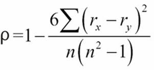
This formula shows us that we'll be summing the differences in rank, and , for all of the pairs of observed values. The Python version of this depends on the sum() and len() functions, as follows:

def rank_corr(pairs):

ranked= rank_xy(pairs)

sum_d_2 = sum((r.r_x - r.r_y)**2 for r in ranked)

n = len(pairs)

return 1-6*sum_d_2/(n*(n**2-1))

We've created Rank_XY objects for each pair. Given this, we can then subtract the r_x and r_y values from those pairs to compare their difference. We can then square and sum the differences.

A good article on statistics will provide detailed guidance on what the coefficient means. A value around 0 means that there is no correlation between the data ranks of the two series of data points. A scatter plot shows a random scattering of points. A value around +1 or -1 indicates a strong relationship between the two values. A graph shows a clear line or curve.

The following is an example based on Anscombe's Quartet series I:

>>> data = (Pair(x=10.0, y=8.04), Pair(x=8.0, y=6.95), …, Pair(x=5.0, y=5.68))

>>> round(rank_corr( data ), 3)

0.818

For this particular data set, the correlation is strong.

In Chapter 4, Working with Collections, we showed how to compute the Pearson correlation coefficient. The function we showed, corr(), worked with two separate sequences of values. We can use it with our sequence of Pair objects as follows:

import ch04_ex4

def pearson_corr(pairs):

X = tuple(p.x for p in pairs)

Y = tuple(p.y for p in pairs)

return ch04_ex4.corr(X, Y)

We've unwrapped the Pair objects to get the raw values that we can use with the existing corr() function. This provides a different correlation coefficient. The Pearson value is based on how well the standardized values compare between two sequences. For many data sets, the difference between the Pearson and Spearman correlations is relatively small. For some datasets, however, the differences can be quite large.

To see the importance of having multiple statistical tools for exploratory data analysis, compare the Spearman and Pearson correlations for the four sets of data in the Anscombe's Quartet.

Polymorphism and Pythonic pattern matching

Some functional programming languages offer clever approaches to working with statically typed function definitions. The issue is that many functions we'd like to write are entirely generic with respect to data type. For example, most of our statistical functions are identical for integer or floating-point numbers, as long as division returns a value that is a subclass of numbers.Real (for example, Decimal, Fraction, or float). In order to make a single generic definition work for multiple data types, sophisticated type or pattern-matching rules are used by the compiler.

Instead of the (possibly) complex features of statically typed functional languages, Python changes the issue using dynamic selection of the final implementation of an operator based on the data types being used. This means that a compiler doesn't certify that our functions are expecting and producing the proper data types. We generally rely on unit testing for this.

In Python, we're effectively writing generic definitions because the code isn't bound to any specific data type. The Python runtime will locate the appropriate operations using a simple set of matching rules. The 3.3.7 Coercion rules section of the language reference manual and the numbers module in the library provide details on how this mapping from operation to special method name works.

In rare cases, we might need to have different behavior based on the types of the data elements. We have two ways to tackle this; they are as follows:

· We can use the isinstance() function to distinguish the different cases

· We can create our own subclass of numbers.Number or tuple and implement a proper polymorphic special method names

In some cases, we'll actually need to do both so that we can include appropriate data type conversions.

When we look back at the ranking example in the previous section, we're tightly bound to the idea of applying rank-ordering to simple pairs. While this is the way the Spearman correlation is defined, we might have a multivariate dataset and have a need to do rank-order correlation among all the variables.

The first thing we'll need to do is generalize our idea of rank-order information. The following is a namedtuple that handles a tuple of ranks and a tuple of raw data:

Rank_Data = namedtuple("Rank_Data", ("rank_seq", "raw"))

For any specific piece of Rank_Data, such as r, we can use r.rank_seq[0] to get a specific ranking and r.raw to get the original observation.

We'll add some syntactic sugar to our ranking function. In many previous examples, we've required either an iterable or a collection. The for statement is graceful about working with either one. However, we don't always use the for statement, and for some functions, we've had to explicitly use iter() to make an iterable out of a collection. We can handle this situation with a simple isinstance() check, as shown in the following code snippet:

def some_function(seq_or_iter):

if not isinstance(seq_or_iter,collections.abc.Iterator):

yield from some_function(iter(seq_or_iter), key)

return

# Do the real work of the function using the iterable

We've included a type check to handle the small difference between the two collections, which doesn't work with next() and an iterable, which supports next().

In the context of our rank-ordering function, we will use this variation on the design pattern:

def rank_data(seq_or_iter, key=lambda obj:obj):

# Not a sequence? Materialize a sequence object

if isinstance(seq_or_iter, collections.abc.Iterator):

yield from rank_data(tuple(seq_or_iter), key)

data = seq_or_iter

head= seq_or_iter[0]

# Convert to Rank_Data and process.

if not isinstance(head, Rank_Data):

ranked= tuple(Rank_Data((),d) for d in data)

for r, rd in rerank(ranked, key):

yield Rank_Data(rd.rank_seq+(r,), rd.raw)

return

# Collection of Rank_Data is what we prefer.

for r, rd in rerank(data, key):

yield Rank_Data(rd.rank_seq+(r,), rd.raw)

We've decomposed the ranking into three cases for three different types of data. We're forced it to do this when the different kinds of data aren't polymorphic subclasses of a common superclass. The following are the three cases:

· Given an iterable (without a usable __getitem__() method), we'll materialize a tuple that we can work with

· Given a collection of some unknown type of data, we'll wrap the unknown objects into Rank_Data tuples

· Finally, given a collection of Rank_Data tuples, we'll add yet another ranking to the tuple of ranks inside the each Rank_Data container

This relies on a rerank() function that inserts and returns another ranking into the Rank_Data tuple. This will build up a collection of individual rankings from a complex record of raw data values. The rerank() function follows a slightly different design than the example of the rank() function shown previously.

This version of the algorithm uses sorting instead of creating a groups in a objects like Counter object:

def rerank(rank_data_collection, key):

sorted_iter= iter(sorted( rank_data_collection, key=lambda obj: key(obj.raw)))

head = next(sorted_iter)

yield from ranker(sorted_iter, 0, [head], key)

We've started by reassembling a single, sortable collection from the head and the data iterator. In the context in which this is used, we can argue that this is a bad idea.

This function relies on two other functions. They can be declared within the body of rerank(). We'll show them separately. The following is the ranker, which accepts an iterable, a base rank number, a collection of values with the same rank, and a key:

def ranker(sorted_iter, base, same_rank_seq, key):

"""Rank values from a sorted_iter using a base rank value.

If the next value's key matches same_rank_seq, accumulate those.

If the next value's key is different, accumulate same rank values

and start accumulating a new sequence.

"""

try:

value= next(sorted_iter)

except StopIteration:

dups= len(same_rank_seq)

yield from yield_sequence((base+1+base+dups)/2, iter(same_rank_seq))

return

if key(value.raw) == key(same_rank_seq[0].raw):

yield from ranker(sorted_iter, base, same_rank_seq+[value], key)

else:

dups= len(same_rank_seq)

yield from yield_sequence( (base+1+base+dups)/2, iter(same_rank_seq))

yield from ranker(sorted_iter, base+dups, [value], key)

We've extracted the next item from the iterable collection of sorted values. If this fails, there is no next item, and we need to emit the final collection of equal-valued items in the same_rank_seq sequence. If this works, then we need to use the key() function to see whether the next item, which is a value, has the same key as the collection of equal-ranked items. If the key is the same, the overall value is defined recursively; the reranking is the rest of the sorted items, the same base value for the rank, a larger collection ofsame_rank items, and the same key() function.

If the next item's key doesn't match the sequence of equal-valued items, the result is a sequence of equal-valued items. This will be followed by the reranking of the rest of the sorted items, a base value incremented by the number of equal-valued items, a fresh list of equal-rank items with just the new value, and the same key extraction function.

This depends on the yield_sequence() function, which looks as follows:

def yield_sequence(rank, same_rank_iter):

head= next(same_rank_iter)

yield rank, head

yield from yield_sequence(rank, same_rank_iter)

We've written this in a way that emphasizes the recursive definition. We don't really need to extract the head, emit it, and then recursively emit the remaining items. While a single for statement might be shorter, it's sometimes more clear to emphasize the recursive structure that has been optimized into a for loop.

The following are some examples of using this function to rank (and rerank) data. We'll start with a simple collection of scalar values:

>>> scalars= [0.8, 1.2, 1.2, 2.3, 18]

>>> list(ranker(scalars))

[Rank_Data(rank_seq=(1.0,), raw=0.8), Rank_Data(rank_seq=(2.5,), raw=1.2), Rank_Data(rank_seq=(2.5,), raw=1.2), Rank_Data(rank_seq=(4.0,), raw=2.3), Rank_Data(rank_seq=(5.0,), raw=18)]

Each value becomes the raw attribute of a Rank_Data object.

When we work with a slightly more complex object, we can also have multiple rankings. The following is a sequence of two tuples:

>>> pairs= ((2, 0.8), (3, 1.2), (5, 1.2), (7, 2.3), (11, 18))

>>> rank_x= tuple(ranker(pairs, key=lambda x:x[0] ))

>>> rank_x

(Rank_Data(rank_seq=(1.0,), raw=(2, 0.8)), Rank_Data(rank_seq=(2.0,), raw=(3, 1.2)), Rank_Data(rank_seq=(3.0,), raw=(5, 1.2)), Rank_Data(rank_seq=(4.0,), raw=(7, 2.3)), Rank_Data(rank_seq=(5.0,), raw=(11, 18)))

>>> rank_xy= (ranker(rank_x, key=lambda x:x[1] ))

>>> tuple(rank_xy)

(Rank_Data(rank_seq=(1.0, 1.0), raw=(2, 0.8)),Rank_Data(rank_seq=(2.0, 2.5), raw=(3, 1.2)), Rank_Data(rank_seq=(3.0, 2.5), raw=(5, 1.2)), Rank_Data(rank_seq=(4.0, 4.0), raw=(7, 2.3)), Rank_Data(rank_seq=(5.0, 5.0), raw=(11, 18)))

Here, we defined a collection of pairs. Then, we ranked the two tuples, assigning the sequence of Rank_Data objects to the rank_x variable. We then ranked this collection of Rank_Data objects, creating a second rank value and assigning the result to the rank_xyvariable.

The resulting sequence can be used to a slightly modified rank_corr() function to compute the rank correlations of any of the available values in the rank_seq attribute of the Rank_Data objects. We'll leave this modification as an exercise for the readers.

Summary

In this chapter, we looked at different ways to use namedtuple objects to implement more complex data structures. The essential features of a namedtuple are a good fit with functional design. They can be created with a creation function and accessed by position as well as name.

We looked at how to use immutable namedtuples instead of stateful object definitions. The core technique was to wrap an object in an immutable tuple to provide additional attribute values.

We also looked at ways to handle multiple data types in Python. For most arithmetic operations, Python's internal method dispatch locates proper implementations. To work with collections, however, we might want to handle iterators and sequences slightly differently.

In the next two chapters, we'll look at the itertools module. This library module provides a number of functions that help us work with iterators in sophisticated ways. Many of these tools are examples of higher-order functions. They can help make a functional design stay succinct and expressive.