Python and HDF5 (2013)
Chapter 2. Getting Started
HDF5 Basics
Before we jump into Python code examples, it’s useful to take a few minutes to address how HDF5 itself is organized. Figure 2-1 shows a cartoon of the various logical layers involved when using HDF5. Layers shaded in blue are internal to the library itself; layers in green represent software that uses HDF5.
Most client code, including the Python packages h5py and PyTables, uses the native C API (HDF5 is itself written in C). As we saw in the introduction, the HDF5 data model consists of three main public abstractions: datasets (see Chapter 3), groups (see Chapter 5), and attributes (seeChapter 6)in addition to a system to represent types. The C API (and Python code on top of it) is designed to manipulate these objects.
HDF5 uses a variety of internal data structures to represent groups, datasets, and attributes. For example, groups have their entries indexed using structures called “B-trees,” which make retrieving and creating group members very fast, even when hundreds of thousands of objects are stored in a group (see How Groups Are Actually Stored). You’ll generally only care about these data structures when it comes to performance considerations. For example, when using chunked storage (see Chapter 4), it’s important to understand how data is actually organized on disk.
The next two layers have to do with how your data makes its way onto disk. HDF5 objects all live in a 1D logical address space, like in a regular file. However, there’s an extra layer between this space and the actual arrangement of bytes on disk. HDF5 drivers take care of the mechanics of writing to disk, and in the process can do some amazing things.
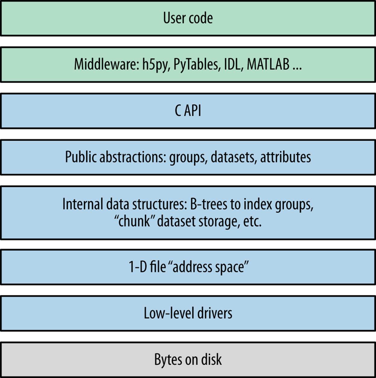
Figure 2-1. The HDF5 library: blue represents components inside the HDF5 library; green represents “client” code that calls into HDF5; gray represents resources provided by the operating system.
For example, the HDF5 core driver lets you use files that live entirely in memory and are blazingly fast. The family driver lets you split a single file into regularly sized pieces. And the mpio driver lets you access the same file from multiple parallel processes, using the Message Passing Interface (MPI) library (MPI and Parallel HDF5). All of this is transparent to code that works at the higher level of groups, datasets, and attributes.
Setting Up
That’s enough background material for now. Let’s get started with Python! But which Python?
Python 2 or Python 3?
A big shift is under way in the Python community. Over the years, Python has accumulated a number of features and misfeatures that have been deemed undesirable. Examples range from packages that use inconsistent naming conventions all the way to deficiencies in how strings are handled. To address these issues, it was decided to launch a new major version (Python 3) that would be freed from the “baggage” of old decisions in the Python 2 line.
Python 2.7, the most recent minor release in the Python series, will also be the last 2.X release. Although it will be updated with bug fixes for an extended period of time, new Python code development is now carried out exclusively on the 3.X line. The NumPy package, h5py, PyTables, and many other packages now support Python 3. While (in my opinion) it’s a little early to recommend that newcomers start with Python 3, the future is clear.
So at the moment, there are two major versions of Python widely deployed simultaneously. Since most people in the Python community are used to Python 2, the examples in this book are also written for Python 2. For the most part, the differences are minor; for example, on Python 3, the syntax for print is print(foo), instead of print foo. Wherever incompatibilities are likely to occur (mainly with string types and certain dictionary-style methods), these will be noted in the text.
“Porting” code to Python 3 isn’t actually that hard; after all, it’s still Python. Some of the most valuable features in Python 3 are already present in Python 2.7. A free tool is also available (2to3) that can accomplish most of the mechanical changes, for example changing print statements toprint() function calls. Check out the migration guide (and the 2to3 tool) at http://www.python.org.
Code Examples
To start with, most of the code examples will follow this form:
>>> a = 1.0
>>> print a
1.0
Or, since Python prints objects by default, an even simpler form:
>>> a
1.0
Lines starting with >>> represent input to Python (>>> being the default Python prompt); other lines represent output. Some of the longer examples, where the program output is not shown, omit the >>> in the interest of clarity.
Examples intended to be run from the command line will start with the Unix-style "$" prompt:
$ python --version
Python 2.7.3
Finally, to avoid cluttering up the examples, most of the code snippets you’ll find here will assume that the following packages have been imported:
>>> import numpy as np # Provides array object and data type objects
>>> import h5py # Provides access to HDF5
NumPy
“NumPy” is the standard numerical-array package in the Python world. This book assumes that you have some experience with NumPy (and of course Python itself), including how to use array objects.
Even if you’ve used NumPy before, it’s worth reviewing a few basic facts about how arrays work. First, NumPy arrays all have a fixed data type or “dtype,” represented by dtype objects. For example, let’s create a simple 10-element integer array:
>>> arr = np.arange(10)
>>> arr
array([0, 1, 2, 3, 4, 5, 6, 7, 8, 9])
The data type of this array is given by arr.dtype:
>>> arr.dtype
dtype('int32')
These dtype objects are how NumPy communicates low-level information about the type of data in memory. For the case of our 10-element array of 4-byte integers (32-bit or “int32” in NumPy lingo), there is a chunk of memory somewhere 40 bytes long that holds the values 0 through 9. Other code that receives the arr object can inspect the dtype object to figure out what the memory contents represent.
NOTE
The preceding example might print dtype('int64') on your system. All this means is that the default integer size available to Python is 64 bits long, instead of 32 bits.
HDF5 uses a very similar type system; every “array” or dataset in an HDF5 file has a fixed type represented by a type object. The h5py package automatically maps the HDF5 type system onto NumPy dtypes, which among other things makes it easy to interchange data with NumPy.Chapter 3 goes into more detail about this process.
Slicing is another core feature of NumPy. This means accessing portions of a NumPy array. For example, to extract the first four elements of our array arr:
>>> out = arr[0:4]
>>> out
array([0, 1, 2, 3])
You can also specify a “stride” or steps between points in the slice:
>>> out = arr[0:4:2]
>>> out
array([0, 2])
When talking to HDF5, we will borrow this “slicing” syntax to allow loading only portions of a dataset.
In the NumPy world, slicing is implemented in a clever way, which generally creates arrays that refer to the data in the original array, rather than independent copies. For example, the preceding out object is likely a “view” onto the original arr array. We can test this:
>>> out[:] = 42
>>> out
array([42, 42])
>>> arr
array([42, 1, 42, 3, 4, 5, 6, 7, 8, 9])
This means slicing is generally a very fast operation. But you should be careful to explicitly create a copy if you want to modify the resulting array without your changes finding their way back to the original:
>>> out2 = arr[0:4:2].copy()
CAUTION
Forgetting to make a copy before modifying a “slice” of the array is a very common mistake, especially for people used to environments like IDL. If you’re new to NumPy, be careful!
As we’ll see later, thankfully this doesn’t apply to slices read from HDF5 datasets. When you read from the file, since the data is on disk, you will always get a copy.
HDF5 and h5py
We’ll use the “h5py” package to talk to HDF5. This package contains high-level wrappers for the HDF5 objects of files, groups, datasets, and attributes, as well as extensive low-level wrappers for the HDF5 C data structures and functions. The examples in this book assume h5py version 2.2.0 or later, which you can get at http://www.h5py.org.
You should note that h5py is not the only commonly used package for talking to HDF5. PyTables is a scientific database package based on HDF5 that adds dataset indexing and an additional type system. Since we’ll be talking about native HDF5 constructs, we’ll stick to h5py, but I strongly recommend you also check out PyTables if those features interest you.
If you’re on Linux, it’s generally a good idea to install the HDF5 library via your package manager. On Windows, you can download an installer from http://www.h5py.org, or use one of the many distributions of Python that include HDF5/h5py, such as PythonXY, Anaconda from Continuum Analytics, or Enthought Python Distribution.
IPython
Apart from NumPy and h5py/HDF5 itself, IPython is a must-have component if you’ll be doing extensive analysis or development with Python. At its most basic, IPython is a replacement interpreter shell that adds features like command history and Tab-completion for object attributes. It also has tons of additional features for parallel processing, MATLAB-style “notebook” display of graphs, and more.
The best way to explore the features in this book is with an IPython prompt open, following along with the examples. Tab-completion alone is worth it, because it lets you quickly see the attributes of modules and objects. The h5py package is specifically designed to be “explorable” in this sense. For example, if you want to discover what properties and methods exist on the File object (see Your First HDF5 File), type h5py.File. and bang the Tab key:
>>> h5py.File.<TAB>
h5py.File.attrs h5py.File.get h5py.File.name
h5py.File.close h5py.File.id h5py.File.parent
h5py.File.copy h5py.File.items h5py.File.ref
h5py.File.create_dataset h5py.File.iteritems h5py.File.require_dataset
h5py.File.create_group h5py.File.iterkeys h5py.File.require_group
h5py.File.driver h5py.File.itervalues h5py.File.userblock_size
h5py.File.fid h5py.File.keys h5py.File.values
h5py.File.file h5py.File.libver h5py.File.visit
h5py.File.filename h5py.File.mode h5py.File.visititems
h5py.File.flush h5py.File.mro
To get more information on a property or method, use ? after its name:
>>> h5py.File.close?
Type: instancemethod
Base Class: <type 'instancemethod'>
String Form:<unbound method File.close>
Namespace: Interactive
File: /usr/local/lib/python2.7/dist-packages/h5py/_hl/files.py
Definition: h5py.File.close(self)
Docstring: Close the file. All open objects become invalid
NOTE
By default, IPython will save the output of your statements in special hidden variables. This is generally OK, but can be surprising if it hangs on to an HDF5 object you thought was discarded, or a big array that eats up memory. You can turn this off by setting the IPython configuration value cache_size to 0. See the docs at http://ipython.org for more information.
Timing and Optimization
For performance testing, we’ll use the timeit module that ships with Python. Examples using timeit will assume the following import:
>>> from timeit import timeit
The timeit function takes a (string or callable) command to execute, and an optional number of times it should be run. It then prints the total time spent running the command. For example, if we execute the “wait” function time.sleep five times:
>>> import time
>>> timeit("time.sleep(0.1)", number=5)
0.49967818316434887
If you’re using IPython, there’s a similar built-in “magic” function called %timeit that runs the specified statement a few times, and reports the lowest execution time:
>>> %timeit time.sleep(0.1)
10 loops, best of 3: 100 ms per loop
We’ll stick with the regular timeit function in this book, in part because it’s provided by the Python standard library.
Since people using HDF5 generally deal with large datasets, performance is always a concern. But you’ll notice that optimization and benchmarking discussions in this book don’t go into great detail about things like cache hits, data conversion rates, and so forth. The design of the h5py package, which this book uses, leaves nearly all of that to HDF5. This way, you benefit from the hundreds of man years of work spent on tuning HDF5 to provide the highest performance possible.
As an application builder, the best thing you can do for performance is to use the API in a sensible way and let HDF5 do its job. Here are some suggestions:
1. Don’t optimize anything unless there’s a demonstrated performance problem. Then, carefully isolate the misbehaving parts of the code before changing anything.
2. Start with simple, straightforward code that takes advantage of the API features. For example, to iterate over all objects in a file, use the Visitor feature of HDF5 (see Multilevel Iteration with the Visitor Pattern) rather than cobbling together your own approach.
3. Do “algorithmic” improvements first. For example, when writing to a dataset (see Chapter 3), write data in reasonably sized blocks instead of point by point. This lets HDF5 use the filesystem in an intelligent way.
4. Make sure you’re using the right data types. For example, if you’re running a compute-intensive program that loads floating-point data from a file, make sure that you’re not accidentally using double-precision floats in a calculation where single precision would do.
5. Finally, don’t hesitate to ask for help on the h5py or NumPy/Scipy mailing lists, Stack Overflow, or other community sites. Lots of people are using NumPy and HDF5 these days, and many performance problems have known solutions. The Python community is very welcoming.
The HDF5 Tools
We’ll be creating a number of files in later chapters, and it’s nice to have an independent way of seeing what they contain. It’s also a good idea to inspect files you create professionally, especially if you’ll be using them for archiving or sharing them with colleagues. The earlier you can detect the use of an incorrect data type, for example, the better off you and other users will be.
HDFView
HDFView is a free graphical browser for HDF5 files provided by the HDF Group. It’s a little basic, but is written in Java and therefore available on Windows, Linux, and Mac. There’s a built-in spreadsheet-like browser for data, and basic plotting capabilities.
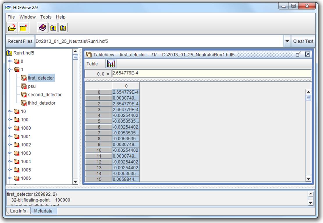
Figure 2-2. HDFView
Figure 2-2 shows the contents of an HDF5 file with multiple groups in the left-hand pane. One group (named “1”) is open, showing the datasets it contains; likewise, one dataset is opened, with its contents displayed in the grid view to the right.
HDFView also lets you inspect attributes of datasets and groups, and supports nearly all the data types that HDF5 itself supports, with the exception of certain variable-length structures.
ViTables
Figure 2-3 shows the same HDF5 file open in ViTables, another free graphical browser. It’s optimized for dealing with PyTables files, although it can handle generic HDF5 files perfectly well. One major advantage of ViTables is that it comes preinstalled with such Python distributions asPythonXY, so you may already have it.
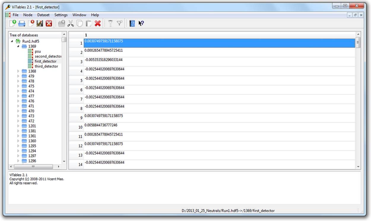
Figure 2-3. ViTables
Command Line Tools
If you’re used to the command line, it’s definitely worth installing the HDF command-line tools. These are generally available through a package manager; if not, you can get them at www.hdfgroup.org. Windows versions are also available.
The program we’ll be using most in this book is called h5ls, which as the name suggests lists the contents of a file. Here’s an example, in which h5ls is applied to a file containing a couple of datasets and a group:
$ h5ls demo.hdf5
array Dataset {10}
group Group
scalar Dataset {SCALAR}
We can get a little more useful information by using the option combo -vlr, which prints extended information and also recursively enters groups:
$ h5ls -vlr demo.hdf5
/ Group
Location: 1:96
Links: 1
/array Dataset {10/10}
Location: 1:1400
Links: 1
Storage: 40 logical bytes, 40 allocated bytes, 100.00% utilization
Type: native int
/group Group
Location: 1:1672
Links: 1
/group/subarray Dataset {2/2, 2/2}
Location: 1:1832
Links: 1
Storage: 16 logical bytes, 16 allocated bytes, 100.00% utilization
Type: native int
/scalar Dataset {SCALAR}
Location: 1:800
Links: 1
Storage: 4 logical bytes, 4 allocated bytes, 100.00% utilization
Type: native int
That’s a little more useful. We can see that the object at /array is of type “native int,” and is a 1D array 10 elements long. Likewise, there’s a dataset inside the group named group that is 2D, also of type native int.
h5ls is great for inspecting metadata like this. There’s also a program called h5dump, which prints data as well, although in a more verbose format:
$ h5dump demo.hdf5
HDF5 "demo.hdf5" {
GROUP "/" {
DATASET "array" {
DATATYPE H5T_STD_I32LE
DATASPACE SIMPLE { ( 10 ) / ( 10 ) }
DATA {
(0): 0, 1, 2, 3, 4, 5, 6, 7, 8, 9
}
}
GROUP "group" {
DATASET "subarray" {
DATATYPE H5T_STD_I32LE
DATASPACE SIMPLE { ( 2, 2 ) / ( 2, 2 ) }
DATA {
(0,0): 2, 2,
(1,0): 2, 2
}
}
}
DATASET "scalar" {
DATATYPE H5T_STD_I32LE
DATASPACE SCALAR
DATA {
(0): 42
}
}
}
}
Your First HDF5 File
Before we get to groups and datasets, let’s start by exploring some of the capabilities of the File object, which will be your entry point into the world of HDF5.
Here’s the simplest possible program that uses HDF5:
>>> f = h5py.File("name.hdf5")
>>> f.close()
The File object is your starting point; it has methods that let you create new datasets or groups in the file, as well as more pedestrian properties such as .filename and .mode.
Speaking of .mode, HDF5 files support the same kind of read/write modes as regular Python files:
>>> f = h5py.File("name.hdf5", "w") # New file overwriting any existing file
>>> f = h5py.File("name.hdf5", "r") # Open read-only (must exist)
>>> f = h5py.File("name.hdf5", "r+") # Open read-write (must exist)
>>> f = h5py.File("name.hdf5", "a") # Open read-write (create if doesn't exist)
There’s one additional HDF5-specific mode, which can save your bacon should you accidentally try to overwrite an existing file:
>>> f = h5py.File("name.hdf5", "w-")
This will create a new file, but fail if a file of the same name already exists. For example, if you’re performing a long-running calculation and don’t want to risk overwriting your output file should the script be run twice, you could open the file in w- mode:
>>> f = h5py.File("important_file.hdf5", "w-")
>>> f.close()
>>> f = h5py.File("important_file.hdf5", "w-")
IOError: unable to create file (File accessability: Unable to open file)
By the way, you’re free to use Unicode filenames! Just supply a normal Unicode string and it will transparently work, assuming the underlying operating system supports the UTF-8 encoding:
>>> name = u"name_eta_\u03b7"
>>> f = h5py.File(name)
>>> print f.filename
name_eta_η
NOTE
You might wonder what happens if your program crashes with open files. If the program exits with a Python exception, don’t worry! The HDF library will automatically close every open file for you when the application exits.
Use as a Context Manager
One of the coolest features introduced in Python 2.6 is support for context managers. These are objects with a few special methods called on entry and exit from a block of code, using the with statement. The classic example is the built-in Python file object:
>>> with open("somefile.txt", "w") as f:
... f.write("Hello!")
The preceding code opens a brand-new file object, which is available in the code block with the name f. When the block exits, the file is automatically closed (even if an exception occurs!).
The h5py.File object supports exactly this kind of use. It’s a great way to make sure the file is always properly closed, without wrapping everything in try/except blocks:
>>> with h5py.File("name.hdf5", "w") as f:
... print f["missing_dataset"]
KeyError: "unable to open object (Symbol table: Can't open object)"
>>> print f
<Closed HDF5 file>
File Drivers
File drivers sit between the filesystem and the higher-level world of HDF5 groups, datasets, and attributes. They deal with the mechanics of mapping the HDF5 “address space” to an arrangement of bytes on disk. Typically you won’t have to worry about which driver is in use, as the default driver works well for most applications.
The great thing about drivers is that once the file is opened, they’re totally transparent. You just use the HDF5 library as normal, and the driver takes care of the storage mechanics.
Here are a couple of the more interesting ones, which can be helpful for unusual problems.
core driver
The core driver stores your file entirely in memory. Obviously there’s a limit to how much data you can store, but the trade-off is blazingly fast reads and writes. It’s a great choice when you want the speed of memory access, but also want to use the HDF5 structures. To enable, set thedriver keyword to "core":
>>> f = h5py.File("name.hdf5", driver="core")
You can also tell HDF5 to create an on-disk “backing store” file, to which the file image is saved when closed:
>>> f = h5py.File("name.hdf5", driver="core", backing_store=True)
By the way, the backing_store keyword will also tell HDF5 to load any existing image from disk when you open the file. So if the entire file will fit in memory, you need to read and write the image only once; things like dataset reads and writes, attribute creation, and so on, don’t take any disk I/O at all.
family driver
Sometimes it’s convenient to split a file up into multiple images, all of which share a certain maximum size. This feature was originally implemented to support filesystems that couldn’t handle file sizes above 2GB.
>>> # Split the file into 1-GB chunks
>>> f = h5py.File("family.hdf5", driver="family", memb_size=1024**3)
The default for memb_size is 231-1, in keeping with the historical origins of the driver.
mpio driver
This driver is the heart of Parallel HDF5. It lets you access the same file from multiple processes at the same time. You can have dozens or even hundreds of parallel computing processes, all of which share a consistent view of a single file on disk.
Using the mpio driver correctly can be tricky. Chapter 9 covers both the details of this driver and best practices for using HDF5 in a parallel environment.
The User Block
One interesting feature of HDF5 is that files may be preceeded by arbitrary user data. When a file is opened, the library looks for the HDF5 header at the beginning of the file, then 512 bytes in, then 1024, and so on in powers of 2. Such space at the beginning of the file is called the “user block,” and you can store whatever data you want there.
The only restrictions are on the size of the block (powers of 2, and at least 512), and that you shouldn’t have the file open in HDF5 when writing to the user block. Here’s an example:
>>> f = h5py.File("userblock.hdf5", "w", userblock_size=512)
>>> f.userblock_size # Would be 0 if no user block present
512
>>> f.close()
>>> with open("userblock.hdf5", "rb+") as f: # Open as regular Python file
... f.write("a"*512)
Let’s move on to the first major object in the HDF5 data model, one that will be familiar to users of the NumPy array type: datasets.