DOING MATH WITH PYTHON Use Programming to Explore Algebra, Statistics, Calculus, and More! (2015)

In this chapter, we’ll start by learning how we can make our programs understand and manipulate sets of numbers. We’ll then see how sets can help us understand basic concepts in probability. Finally, we’ll learn about generating random numbers to simulate random events. Let’s get started!

What’s a Set?

A set is a collection of distinct objects, often called elements or members. Two characteristics of a set make it different from just any collection of objects. A set is “well defined,” meaning the question “Is a particular object in this collection?” always has a clear yes or no answer, usually based on a rule or some given criteria. The second characteristic is that no two members of a set are the same. A set can contain anything—numbers, people, things, words, and so on.

Let’s walk through some basic properties of sets as we learn how to work with sets in Python using SymPy.

Set Construction

In mathematical notation, you represent a set by writing the set members enclosed in curly brackets. For example, {2, 4, 6} represents a set with 2, 4, and 6 as its members. To create a set in Python, we can use the FiniteSet class from the sympy package, as follows:

>>> from sympy import FiniteSet
>>> s = FiniteSet(2, 4, 6)
>>> s
{2, 4, 6}

Here, we first import the FiniteSet class from SymPy and then create an object of this class by passing in the set members as arguments. We assign the label s to the set we just created.

We can store different types of numbers—including integers, floating point numbers, and fractions—in the same set:

>>> from sympy import FiniteSet
>>> from fractions import Fraction
>>> s = FiniteSet(1, 1.5, Fraction(1, 5))
>>> s
{1/5, 1, 1.5}

The cardinality of a set is the number of members in the set, which you can find by using the len() function:

>>> s = FiniteSet(1, 1.5, 3)
>>> len(s)
3

Checking Whether a Number Is in a Set

To check whether a number is a member of an existing set, use the in operator. This operator asks Python, “Is this number in this set?” It returns True if the number belongs to the set and False if it doesn’t. If, for example, we wanted to check whether 4 was in the previous set, we’d do the following:

>>> 4 in s
False

Because 4 is not present in the set, the operator returns False.

Creating an Empty Set

If you want to make an empty set, which is a set that doesn’t have any elements or members, create a FiniteSet object without passing any arguments. The result is an EmptySet object:

>>> s = FiniteSet()
>>> s
EmptySet()

Creating Sets from Lists or Tuples

You can also create a set by passing in a list or a tuple of set members as an argument to FiniteSet:

>>> members = [1, 2, 3]
>>> s = FiniteSet(*members)
>>> s
{1, 2, 3}

Here, instead of passing in the set members directly to FiniteSet, we first stored them in a list, which we called members. Then, we passed the list to FiniteSet using this special Python syntax, which basically translates to creating a FiniteSet object that passes the list members as separate arguments and not as a list. That is, this approach to creating a FiniteSet object is equivalent to FiniteSet(1, 2, 3). We will make use of this syntax when the set members are computed at runtime.

Set Repetition and Order

Sets in Python (like mathematical sets) ignore any repeats of a member, and they don’t keep track of the order of set members. For example, if you create a set from a list that has multiple instances of a number, the number is added to the set only once, and the other instances are discarded:

>>> from sympy import FiniteSet
>>> members = [1, 2, 3, 2]
>>> FiniteSet(*members)
{1, 2, 3}

Here, even though we passed in a list that had two instances of the number 2, the number 2 appears only once in the set created from that list.

In Python lists and tuples, each element is stored in a particular order, but the same is not always true for sets. For example, we can print out each member of a set by iterating through it as follows:

>>> from sympy import FiniteSet
>>> s = FiniteSet(1, 2, 3)
>>> for member in s:
print(member)

2
1
3

When you run this code, the elements could be printed in any possible order. This is because of how sets are stored by Python—it keeps track of what members are in the set, but it doesn’t keep track of any particular order for those members.

Let’s see another example. Two sets are equal when they have the same elements. In Python, you can use the equality operator, ==, to check whether two sets are equal:

>>> from sympy import FiniteSet
>>> s = FiniteSet(3, 4, 5)
>>> t = FiniteSet(5, 4, 3)
>>> s == t
True

Although the members of these two sets appear in different orders, the sets are still equal.

Subsets, Supersets, and Power Sets

A set, s, is a subset of another set, t, if all the members of s are also members of t. For example, the set {1} is a subset of the set {1, 2}. You can check whether a set is a subset of another set using the is_subset() method:

>>> s = FiniteSet(1)
>>> t = FiniteSet(1,2)
>>> s.is_subset(t)
True
>>> t.is_subset(s)
False

Note that an empty set is a subset of every set. Also, any set is a subset of itself, as you can see in the following:

>>> s.is_subset(s)
True
>>> t.is_subset(t)
True

Similarly, a set, t, is said to be a superset of another set, s, if t contains all of the members contained in s. You can check whether one set is a superset of another using the is_superset() method:

>>> s.is_superset(t)
False
>>> t.is_superset(s)
True

The power set of a set, s, is the set of all possible subsets of s. Any set, s, has precisely 2^|s| subsets, where |s| is the cardinality of the set. For example, the set {1, 2, 3} has a cardinality of 3, so it has 2³ or 8 subsets: {} (the empty set), {1}, {2}, {3}, {1, 2}, {2, 3}, {1, 3}, and {1, 2, 3}.

The set of all these subsets form the power set, and we can find the power set using the powerset() method:

>>> s = FiniteSet(1, 2, 3)
>>> ps = s.powerset()
>>> ps
{{1}, {1, 2}, {1, 3}, {1, 2, 3}, {2}, {2, 3}, {3}, EmptySet()}

As the power set is a set itself, you can find its cardinality using the len() function:

>>> len(ps)
8

The cardinality of the power set is 2^|s|, which is 2³ = 8.

Based on our definition of a subset, any two sets with the exact same members would be subsets as well as supersets of each other. By contrast, a set, s, is a proper subset of t only if all the members of s are also in t and t has at least one member that is not in s. So if s = {1, 2, 3}, it’s only a proper subset of t if t contains 1, 2, and 3 plus at least one more member. This would also mean that t is a proper superset of s. You can use the is_proper_subset() method and the is_proper_superset() method to check for these relationships:

>>> from sympy import FiniteSet
>>> s = FiniteSet(1, 2, 3)
>>> t = FiniteSet(1, 2, 3)
>>> s.is_proper_subset(t)
False
>>> t.is_proper_superset(s)
False

Now, if we re-create the set t to include another member, s will be considered a proper subset of t and t a proper superset of s:

>>> t = FiniteSet(1, 2, 3, 4)
>>> s.is_proper_subset(t)
True
>>> t.is_proper_superset(s)
True

COMMON NUMBER SETS

In the first chapter, we learned that there are different kinds of numbers— integers, floating point numbers, fractions, and complex numbers. All these numbers form different sets of numbers, which have special names.

All positive and negative whole numbers form the set of integers. All positive integers form the set of natural numbers (sometimes 0 is included in this set of numbers even though it’s not positive, but sometimes not). This means the set of natural numbers is a proper subset of the set of integers.

The set of rational numbers includes any number that can be expressed as a fraction, which includes all integers, plus any number with a decimal ending that terminates or repeats (including numbers like 1/4 or 0.25, and 1/3 or 0.33333 ...). By contrast, nonrepeating, nonterminating decimal numbers are known as irrational numbers. The square root of 2 and π are both examples of irrational numbers because they go on forever without repeating.

If you put together all the rational and irrational numbers, you get the set of real numbers. But even larger than that is the set of complex numbers, which includes all real numbers and all numbers with an imaginary component.

All of these sets of numbers are infinite sets because they have infinite members. In contrast, the sets we’ve discussed in this chapter have a finite number of members, which is why the SymPy class we’re using is called FiniteSet.

Set Operations

Set operations such as union, intersection, and the Cartesian product allow you to combine sets in certain methodical ways. These set operations are extremely useful in real-world problem-solving situations when we have to consider multiple sets together. Later in this chapter, we’ll see how to use these operations to apply a formula to multiple sets of data and calculate the probabilities of random events.

Union and Intersection

The union of two sets is a set that contains all of the distinct members of the two sets. In set theory, we use the symbol ∪ to refer to the union operation. For example, {1, 2}∪ {2, 3} will result in a new set, {1, 2, 3}. In SymPy, the union of these two sets can be created using the union()method:

>>> from sympy import FiniteSet
>>> s = FiniteSet(1, 2, 3)
>>> t = FiniteSet(2, 4, 6)
>>> s.union(t)
{1, 2, 3, 4, 6}

We find the union of s and t by applying the union method to s and passing in t as an argument. The result is a third set with all the distinct members of the two sets. In other words, each member of this third set is a member of one or both of the first two sets.

The intersection of two sets creates a new set from the elements common to both sets. For example, the intersection of the sets {1, 2} and {2, 3} will result in a new set with the only common element, {2}. Mathematically, this operation is written as {1, 2} ∩ {2, 3}.

In SymPy, use the intersect() method to find the intersection:

>>> s = FiniteSet(1, 2)
>>> t = FiniteSet(2, 3)
>>> s.intersect(t)
{2}

Whereas the union operation finds members that are in one set or another, the intersection operation finds elements that are present in both. Both of these operations can also be applied to more than two sets. For example, here’s how you’d find the union of three sets:

>>> from sympy import FiniteSet
>>> s = FiniteSet(1, 2, 3)
>>> t = FiniteSet(2, 4, 6)
>>> u = FiniteSet(3, 5, 7)
>>> s.union(t).union(u)
{1, 2, 3, 4, 5, 6, 7}

Similarly, here’s how you’d find the intersection of three sets:

>>> s.intersect(t).intersect(u)
EmptySet()

The intersection of the sets s, t, and u turns out to be an empty set because there are no elements that all three sets share.

Cartesian Product

The Cartesian product of two sets creates a set that consists of all possible pairs made by taking an element from each set. For example, the Cartesian product of the sets {1, 2} and {3, 4} is {(1, 3), (1, 4), (2, 3), (2, 4)}. In SymPy, you can find the Cartesian product of two sets by simply using the multiplication operator:

>>> from sympy import FiniteSet
>>> s = FiniteSet(1, 2)
>>> t = FiniteSet(3, 4)
>>> p = s*t
>>> p
{1, 2} x {3, 4}

This takes the Cartesian product of the sets s and t and stores it as p. To actually see each pair in that Cartesian product, we can iterate through and print them out as follows:

>>> for elem in p:
print(elem)
(1, 3)
(1, 4)
(2, 3)
(2, 4)

Each element of the product is a tuple consisting of a member from the first set and a member from the second set.

The cardinality of the Cartesian product is the product of the cardinality of the individual sets. We can demonstrate this in Python:

>>> len(p) == len(s)*len(t)
True

If we apply the exponential operator (**) to a set, we get the Cartesian product of that set times itself the specified number of times.

>>> from sympy import FiniteSet
>>> s = FiniteSet(1, 2)
>>> p = s**3
>>> p
{1, 2} x {1, 2} x {1, 2}

Here, for example, we raised the set s to the power of 3. Because we’re taking the Cartesian product of three sets, this gives us a set of all possible triplets that contain a member of each set:

>>> for elem in p:
print(elem)
(1, 1, 1)
(1, 1, 2)
(1, 2, 1)
(1, 2, 2)
(2, 1, 1)
(2, 1, 2)
(2, 2, 1)
(2, 2, 2)

Finding the Cartesian product of sets is useful for finding all possible combinations of the set members, which we’ll explore next.

Applying a Formula to Multiple Sets of Variables

Consider a simple pendulum of length L. The time period, T, of this pendulum—that is, the amount of time it takes for the pendulum to complete one full swing—is given by the formula

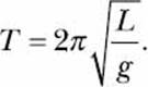
Here, π is the mathematical constant, pi, and g is the local gravitational acceleration, which is around 9.8 m/s² on Earth. Because π and g are constants, the length, L, is the only variable on the right side of the equation that doesn’t have a constant value.

If you wanted to see how the time period of a simple pendulum varies with its length, you’d assume different values for the length and measure the corresponding time period at each of these values using the formula. A typical high school experiment is to compare the time period you get using the preceding formula, which is the theoretical result, to the one you measure in the laboratory, which is the experimental result. For example, let’s choose five different values: 15, 18, 21, 22.5, and 25 (all expressed in centimeters). With Python, we can write a quick program that’ll speed through the calculations for the theoretical results:

from sympy import FiniteSet, pi
➊ def time_period(length):
g = 9.8
T = 2*pi*(length/g)**0.5
return T

if __name__ == '__main__':
➋ L = FiniteSet(15, 18, 21, 22.5, 25)
for l in L:
➌ t = time_period(l/100)
print('Length: {0} cm Time Period: {1:.3f} s'. format(float(l), float(t)))

We first define the function time_period at ➊. This function applies the formula shown earlier to a given length, which is passed in as length. Then, our program defines a set of lengths at ➋ and applies the time_period function to each value at ➌. Notice that when we pass in the length values to time_period, we divide them by 100. This operation converts the lengths from centimeters to meters so that they match the unit of gravitational acceleration, which is expressed in units of meters/second². Finally, we print the calculated time period. When you run the program, you’ll see the following output:

Length: 15.0 cm Time Period: 0.777 s
Length: 18.0 cm Time Period: 0.852 s
Length: 21.0 cm Time Period: 0.920 s
Length: 22.5 cm Time Period: 0.952 s
Length: 25.0 cm Time Period: 1.004 s

Different Gravity, Different Results

Now, imagine we conducted this experiment in three different places— my current location, Brisbane, Australia; the North Pole; and the equator. The force of gravity varies slightly depending on the latitude of your location: it’s a bit lower (approximately 9.78 m/s²) at the equator and higher (9.83 m/s²) at the North Pole. This means we can treat the force of gravity as a variable in our formula, rather than a constant, and calculate results for three different values of gravitational acceleration: {9.8, 9.78, 9.83}.

If we want to calculate the period of a pendulum for each of our five lengths at each of these three locations, a systematic way to work out all of these combinations of the values is to take the Cartesian product, as shown in the following program:

from sympy import FiniteSet, pi

def time_period(length, g):

T = 2*pi*(length/g)**0.5
return T

if __name__ == '__main__':

L = FiniteSet(15, 18, 21, 22.5, 25)
g_values = FiniteSet(9.8, 9.78, 9.83)
➊ print('{0:^15}{1:^15}{2:^15}'.format('Length(cm)', 'Gravity(m/s^2)', 'Time Period(s)'))
➋ for elem in L*g_values:
➌ l = elem[0]
➍ g = elem[1]
t = time_period(l/100, g)

➎ print('{0:^15}{1:^15}{2:^15.3f}'.format(float(l), float(g), float(t)))

At ➋, we take the Cartesian product of our two sets of variables, L and g_values, and we iterate through each resulting combination of values to calculate the time period. Each combination is represented as a tuple, and for each tuple, we extract the first value, the length, at ➌ and the second value, the gravity, at ➍. Then, just as before, we call the time_period() function with these two labels as parameters, and we print the values of length (l), gravity (g), and the corresponding time period (T).

The output is presented in a table to make it easy to follow. The table is formatted by the print statements at ➊ and ➎. The format string {0:^15} {1:^15}{2:^15.3f} creates three fields, each 15 spaces wide, and the ^ symbol centers each entry in each field. In the last field of the printstatement at ➎, '.3f' limits the number of digits after the decimal point to three.

When you run the program, you’ll see the following output:

Length(cm) Gravity(m/s^2) Time Period(s)
15.0 9.78 0.778
15.0 9.8 0.777
15.0 9.83 0.776

18.0 9.78 0.852
18.0 9.8 0.852
18.0 9.83 0.850
21.0 9.78 0.921
21.0 9.8 0.920
21.0 9.83 0.918
22.5 9.78 0.953
22.5 9.8 0.952
22.5 9.83 0.951
25.0 9.78 1.005
25.0 9.8 1.004
25.0 9.83 1.002

This experiment presents a simple scenario where you need all possible combinations of the elements of multiple sets (or a group of numbers). In this type of situation, the Cartesian product is exactly what you need.

Probability

Sets allow us to reason about the basic concepts of probability. We’ll begin with a few definitions:

Experiment The experiment is simply the test we want to perform. We perform the test because we’re interested in the probability of each possible outcome. Rolling a die, flipping a coin, and pulling a card from a deck of cards are all examples of experiments. A single run of an experiment is referred to as a trial.

Sample space All possible outcomes of an experiment form a set known as the sample space, which we’ll usually call S in our formulas. For example, when a six-sided die is rolled once, the sample space is {1, 2, 3, 4, 5, 6}.

Event An event is a set of outcomes that we want to calculate the probability of and that form a subset of the sample space. For example, we might want to know the probability of a particular outcome, like rolling a 3, or the probability of a set of multiple outcomes, such as rolling an even number (either 2, 4, or 6). We’ll use the letter E in our formulas to stand for an event.

If there’s a uniform distribution—that is, if each outcome in the sample space is equally likely to occur—then the probability of an event, P(E), occurring is calculated using the following formula (I’ll talk about nonuniform distributions a bit later in this chapter):

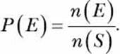
Here, n(E) and n(S) are the cardinality of the sets E, the event, and S, the sample space, respectively. The value of P(E) ranges from 0 to 1, with higher values indicating a higher chance of the event happening.

We can apply this formula to a die roll to calculate the probability of a particular roll—say, 3:

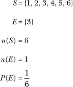
This confirms what was obvious all along: the probability of a particular die roll is 1/6. You could easily do this calculation in your head, but we can use this formula to write the following function in Python that calculates the probability of any event, event, in any sample space, space:

def probability(space, event):
return len(event)/len(space)

In this function, the two arguments space and event—the sample space and event—need not be sets created using FiniteSet. They can also be lists or, for that matter, any other Python object that supports the len() function.

Using this function, let’s write a program to find the probability of a prime number appearing when a 20-sided die is rolled:

def probability(space, event):
return len(event)/len(space)

➊ def check_prime(number):
if number != 1:
for factor in range(2, number):
if number % factor == 0:
return False
else:
return False
return True

if __name__ == '__main__':
➋ space = FiniteSet(*range(1, 21))
primes = []
for num in s:
➌ if check_prime(num):
primes.append(num)
➍ event= FiniteSet(*primes)
p = probability(space, event)

print('Sample space: {0}'.format(space))
print('Event: {0}'.format(event))
print('Probability of rolling a prime: {0:.5f}'.format(p))

We first create a set representing the sample space, space, using the range() function at ➋. To create the event set, we need to find the prime numbers from the sample space, so we define a function, check_prime(), at ➊. This function takes an integer and checks to see whether it’s divisible (with no remainder) by any number between 2 and itself. If so, it returns False. Because a prime number is only divisible by 1 and itself, this function returns True if an integer is prime and False otherwise.

We call this function for each of the numbers in the sample space at ➌ and add the prime numbers to a list, primes. Then, we create our event set, event, from this list at ➍. Finally, we call the probability() function we created earlier. We get the following output when we run the program:

Sample space: {1, 2, 3, ..., 18, 19, 20}
Event: {2, 3, 5, 7, 11, 13, 17, 19}
Probability of rolling a prime: 0.40000

Here, n(E) = 8 and n(S) = 20, so the probability, P, is 0.4.

In our 20-sided die program, we really didn’t need to create the sets; instead, we could have called the probability() function with the sample space and events as lists:

if __name__ == '__main__':
space = range(1, 21)
primes = []
for num in space:
if check_prime(num):
primes.append(num)
p = probability(space, primes)

The probability() function works equally well in this case.

Probability of Event A or Event B

Let’s say we’re interested in two possible events, and we want to find the probability of either one of them happening. For example, going back to a simple die roll, let’s consider the following two events:

A = The number is a prime number.

B = The number is odd.

As it was earlier, the sample space, S, is {1, 2, 3, 4, 5, 6}. Event A can be represented as the subset {2, 3, 5}, the set of prime numbers in the sample space, and event B can be represented as {1, 3, 5}, the odd numbers in the sample space. To calculate the probability of either set of outcomes, we can find the probability of the union of the two sets. In our notation, we could say:

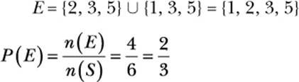
Now let’s perform this calculation in Python:

>>> from sympy import FiniteSet
>>> s = FiniteSet(1, 2, 3, 4, 5, 6)
>>> a = FiniteSet(2, 3, 5)
>>> b = FiniteSet(1, 3, 5)
➊ >>> e = a.union(b)
>>> len(e)/len(s)
0.6666666666666666

We first create a set, s, representing the sample space, followed by the two sets a and b. Then, at ➊, we use the union() method to find the event set, e. Finally, we calculate the probability of the union of the two sets using the earlier formula.

Probability of Event A and Event B

Say you have two events in mind and you want to calculate the chances of both of them happening—for example, the chances that a die roll is both prime and odd. To determine this, you calculate the probability of the intersection of the two event sets:

E = A ∩ B = {2, 3, 5} ∩ {1, 3, 5} = {3, 5}

We can calculate the probability of both A and B happening by using the intersect() method, which is similar to what we did in the previous case:

>>> from sympy import FiniteSet
>>> s = FiniteSet(1, 2, 3, 4, 5, 6)
>>> a = FiniteSet(2, 3, 5)
>>> b = FiniteSet(1, 3, 5)
>>> e = a.intersect(b)
>>> len(e)/len(s)
0.3333333333333333

Generating Random Numbers

Probability concepts allow us to reason about and calculate the chance of an event happening. To actually simulate such events—like a simple dice game—using computer programs, we need a way to generate random numbers.

Simulating a Die Roll

To simulate a six-sided die roll, we need a way to generate a random integer between 1 and 6. The random module in Python’s standard library provides us with various functions to generate random numbers. Two functions that we’ll use in this chapter are the randint() function, which generates a random integer in a given range, and the random() function, which generates a floating point number between 0 and 1. Let’s see a quick example of how the randint() function works:

>>> import random
>>> random.randint(1, 6)
4

The randint() function takes two integers as arguments and returns a random integer that falls between these two numbers (both inclusive). In this example, we passed in the range (1, 6), and it returned the number 4, but if we call it again, we’ll very likely get a different number:

>>> random.randint(1, 6)
6

Calling the randint() function allows us to simulate the roll of our virtual die. Every time we call this function, we’re going to get a number between 1 and 6, just as we would if we were rolling a six-sided die. Note that randint() expects you to supply the lower number first, sorandint(6, 1) isn’t valid.

Can You Roll That Score?

Our next program will simulate a simple die-rolling game, where we keep rolling the six-sided die until we’ve rolled a total of 20:

'''
Roll a die until the total score is 20
'''

import matplotlib.pyplot as plt
import random

target_score = 20

def roll():
return random.randint(1, 6)

if __name__ == '__main__':
score = 0
num_rolls = 0
➊ while score < target_score:
die_roll = roll()
num_rolls += 1
print('Rolled: {0}'.format(die_roll))
score += die_roll

print('Score of {0} reached in {1} rolls'.format(score, num_rolls))

First, we define the same roll() function we created earlier. Then, we use a while loop at ➊ to call this function, keep track of the number of rolls, print the current roll, and add up the total score. The loop repeats until the score reaches 20, and then the program prints the total score and number of rolls.

Here’s a sample run:

Rolled: 6
Rolled: 2
Rolled: 5
Rolled: 1
Rolled: 3
Rolled: 4
Score of 21 reached in 6 rolls

If you run the program several times, you’ll notice that the number of rolls it takes to reach 20 varies.

Is the Target Score Possible?

Our next program is similar, but it’ll tell us whether a certain target score is reachable within a maximum number of rolls:

from sympy import FiniteSet
import random

def find_prob(target_score, max_rolls):

die_sides = FiniteSet(1, 2, 3, 4, 5, 6)
# Sample space
➊ s = die_sides**max_rolls
# Find the event set
if max_rolls > 1:
success_rolls = []
➋ for elem in s:
if sum(elem) >= target_score:
success_rolls.append(elem)
else:
if target_score > 6:
➌ success_rolls = []
else:
success_rolls = []
for roll in die_sides:
➍ if roll >= target_score:
success_rolls.append(roll)
➎ e = FiniteSet(*success_rolls)
# Calculate the probability of reaching target score
return len(e)/len(s)

if __name__ == '__main__':

target_score = int(input('Enter the target score: '))
max_rolls = int(input('Enter the maximum number of rolls allowed: '))

p = find_prob(target_score, max_rolls)
print('Probability: {0:.5f}'.format(p))

When you run this program, it asks for the target score and the maximum number of allowed rolls as input, and then it prints out the probability of achieving that.

Here are two sample executions:

Enter the target score: 25
Enter the maximum number of rolls allowed: 4
Probability: 0.00000

Enter the target score: 25
Enter the maximum number of rolls allowed: 5
Probability: 0.03241

Let’s understand the workings of the find_prob() function, which performs the probability calculation. The sample space here is the Cartesian product, die_sides^max_rolls ➊, where die_sides is the set {1, 2, 3, 4, 5, 6}, representing the numbers on a six-sided die, and max_rolls is the maximum number of die rolls allowed.

The event set is all the sets in the sample space that help us reach this target score. There are two cases here: when the number of turns left is greater than 1 and when we’re in the last turn. For the first case, at ➋, we iterate over each of the tuples in the Cartesian product and add the ones that add up to or exceed target_score in the success_rolls list. The second case is special: our sample space is just the set {1, 2, 3, 4, 5, 6}, and we have only one throw of the die left. If the value of the target score is greater than 6, it isn’t possible to achieve it, and we set success_rolls to be an empty list at ➌. If however, the target_score is less than or equal to 6, we iterate over each possible roll and add the ones that are greater than or equal to the value of target_score at ➍.

At ➎, we calculate the event set, e, from the success_rolls list that we constructed earlier and then return the probability of reaching the target score.

Nonuniform Random Numbers

Our discussions of probability have so far assumed that each of the outcomes in the sample space is equally likely. The random.randint() function, for example, returns an integer in the specified range assuming that each integer is equally likely. We refer to such probability as uniform probability and to random numbers generated by the randint() function as uniform random numbers. Let’s say, however, that we want to simulate a biased coin toss—a loaded coin for which heads is twice as likely to occur as tails. We’d then need a way to generate nonuniform random numbers.

Before we write the program to do so, we’ll review the idea behind it.

Consider a number line with a length of 1 and with two equally divided intervals, as shown in Figure 5-1.

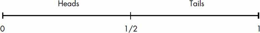
Figure 5-1: A number line with a length of 1 divided into two equal intervals corresponding to the probability of heads or tails on a coin toss

We’ll refer to this line as the probability number line, with each division representing an equally possible outcome—for example, heads or tails upon a fair coin toss. Now, in Figure 5-2, consider a different version of this number line.

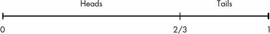
Figure 5-2: A number line with a length of 1 divided into two unequal intervals corresponding to the probability of heads or tails on a biased coin toss

Here, the division corresponding to heads is 2/3 of the total length and the division corresponding to tails is 1/3. This represents the situation of a coin that’s likely to turn up heads in 2/3 of tosses and tails only in 1/3 of tosses. The following Python function will simulate such a coin toss, considering this unequal probability of heads or tails appearing:

import random

def toss():
# 0 -> Heads, 1-> Tails
➊ if random.random() < 2/3:
return 0
else:
return 1

We assume that the function returns 0 to indicate heads and 1 to indicate tails, and then we generate a random number between 0 and 1 at ➊ using the random.random() function. If the generated number is less than 2/3—the probability of flipping heads with our biased coin—the program returns 0; otherwise it returns 1 (tails).

We’ll now see how we can extrapolate the preceding function to simulate a nonuniform event with multiple possible outcomes. Let’s consider a fictional ATM that dispenses a $5, $10, $20, or $50 bill when its button is pressed. The different denominations have varying probabilities of being dispensed, as shown in Figure 5-3.

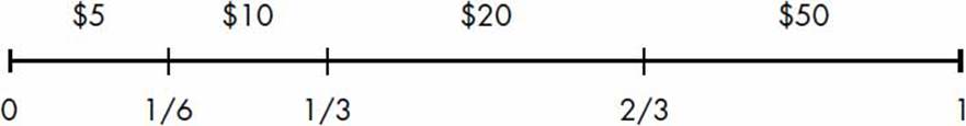
Figure 5-3: A number line with a length of 1 divided into four intervals of different lengths corresponding to the probability of dispensing bills of different denominations

Here, the probability of a $5 bill or $10 bill being dispensed is 1/6, and the probability of a $20 bill or $50 bill being dispensed is 1/3.

We create a list to store the rolling sum of the probabilities, and then we generate a random number between 0 and 1. We start from the left end of the list that stores the sum and return the first index of this list for which the corresponding sum is lesser than or equal to the random number generated. The get_index() function implements this idea:

'''
Simulate a fictional ATM that dispenses dollar bills
of various denominations with varying probability
'''

import random

def get_index(probability):
c_probability = 0
➊ sum_probability = []
for p in probability:
c_probability += p
sum_probability.append(c_probability)
➋ r = random.random()
for index, sp in enumerate(sum_probability):
➌ if r <= sp:
return index
➍ return len(probability)-1

def dispense():

dollar_bills = [5, 10, 20, 50]
probability = [1/6, 1/6, 1/3, 2/3]
bill_index = get_index(probability)
return dollar_bills[bill_index]

We call the get_index() function with a list containing the probability that the event in the corresponding position is expected to occur. We then, at ➊, construct the list sum_probability, where the ith element is the sum of the first i elements in the list probability. That is, the first element in sum_probability is equal to the first element in probability, the second element is equal to the sum of the first two elements in probability, and so on. At ➋, a random number between 0 and 1 is generated using the label r. Next, at ➌, we traverse through sum_probability and return the index of the first element that exceeds r.

The last line of the function, at ➍, takes care of a special case best illustrated through an example. Consider a list of three events with percentages of occurrence each expressed as 0.33. In this case, the list sum_probability would look like [0.33, 0.66, 0.99]. Now, consider that the random number generated, r, is 0.99314. For this value of r, we want the last element in the list of events to be chosen. You may argue that this isn’t exactly right because the last event has a higher than 33 percent chance of being selected. As per the condition at ➌, there’s no element insum_probability that’s greater than r; hence, the function wouldn’t return any index at all. The statement at ➍ takes care of this and returns the last index.

If you call the dispense() function to simulate a large number of dollar bills disbursed by the ATM, you’ll see that the ratio of the number of times each bill appears closely obeys the probability specified. We’ll find this technique useful when creating fractals in the next chapter.

What You Learned

In this chapter, you started by learning how to represent a set in Python. Then, we discussed the various set concepts and you learned about the union, the intersection, and the Cartesian product of sets. You applied some of the set concepts to explore the basics of probability and, finally, learned how to simulate uniform and nonuniform random events in your programs.

Programming Challenges

Next, you have a few programming challenges to solve that’ll give you the opportunity to apply what you’ve learned in this chapter.

#1: Using Venn Diagrams to Visualize Relationships Between Sets

A Venn diagram is an easy way to see the relationship between sets graphically. It tells us how many elements are common between the two sets, how many elements are only in one set, and how many elements are in neither set. Consider a set, A, that represents the set of positive odd numbers less than 20—that is, A = {1, 3, 5, 7, 9, 11, 13, 15, 17, 19}—and consider another set, B, that represents the set of prime numbers less than 20—that is, B = {2, 3, 5, 7, 11, 13, 17, 19}. We can draw Venn diagrams with Python using the matplotlib_venn package (see Appendix A for installation instructions for this package). Once you’ve installed it, you can draw the Venn diagram as follows:

'''
Draw a Venn diagram for two sets
'''

from matplotlib_venn import venn2
import matplotlib.pyplot as plt
from sympy import FiniteSet

def draw_venn(sets):

venn2(subsets=sets)
plt.show()

if __name__ == '__main__':

s1 = FiniteSet(1, 3, 5, 7, 9, 11, 13, 15, 17, 19)
s2 = FiniteSet(2, 3, 5, 7, 11, 13, 17, 19)

draw_venn([s1, s2])

Once we import all the required modules and functions (the venn2() function, matplotlib.pyplot, and the FiniteSet class), all we have to do is create the two sets and then call the venn2() function, using the subsets key-word argument to specify the sets as a tuple.

Figure 5-4 shows the Venn diagram created by the preceding program. The sets A and B share seven common elements, so 7 is written in the common area. Each of the sets also has unique elements, so the number of unique elements—3 and 1, respectively—is written in the individual areas. The labels below the two sets are shown as A and B. You can specify your own labels using the set_labels keyword argument:

>>> venn2(subsets=(a,b), set_labels=('S', 'T'))

This would change the set labels to S and T.

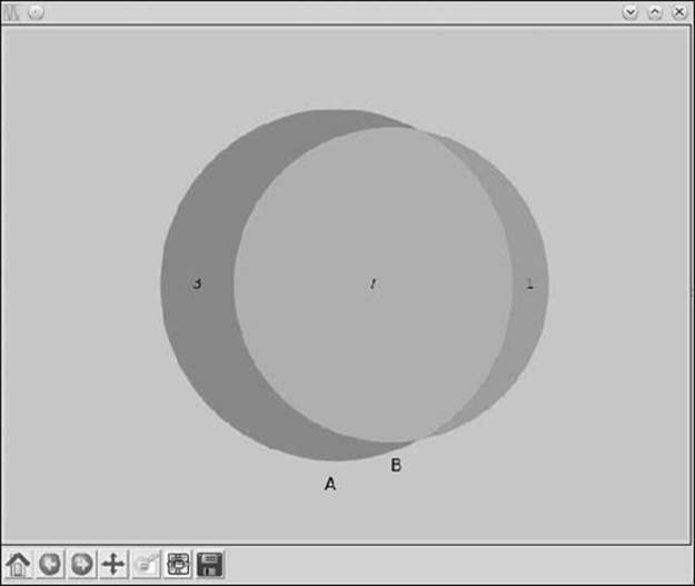
Figure 5-4: Venn diagram showing the relationship between two sets, A and B

For your challenge, imagine you’ve created an online questionnaire asking your classmates the following question: Do you play football, another sport, or no sports? Once you have the results, create a CSV file, sports.csv, as follows:

StudentID,Football,Others
1,1,0
2,1,1
3,0,1
--snip--

Create 20 such rows for the 20 students in your class. The first column is the student ID (the survey isn’t anonymous), the second column has a 1 if the student has marked “football” as the sport they love to play, and the third column has a 1 if the student plays any other sport or none at all. Write a program to create a Venn diagram to depict the summarized results of the survey, as shown in Figure 5-5.

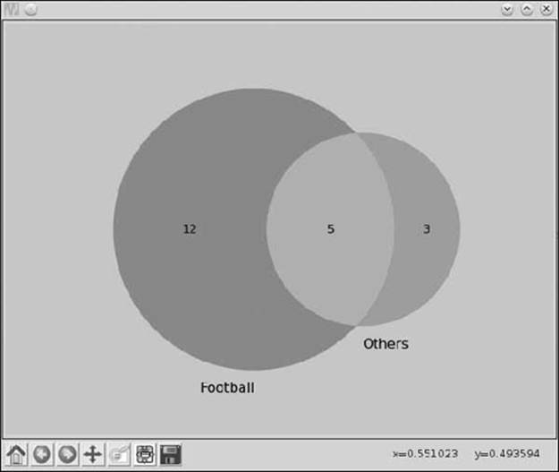
Figure 5-5: A Venn diagram showing the number of students who love to play football and the number who love to play other sports

Depending on the data in the sports.csv file you created, the numbers in each set will vary. The following function reads a CSV file and returns two lists corresponding to the IDs of those students who play football and other sports:

def read_csv(filename):
football = []
others = []
with open(filename) as f:
reader = csv.reader(f)
next(reader)
for row in reader:
if row[1] == '1':
football.append(row[0])
if row[2] == '1':
others.append(row[0])

return football, others

#2: Law of Large Numbers

We’ve referred to a die roll and coin toss as two examples of random events that we can simulate using random numbers. We’ve used the term event to refer to a certain number showing up on a die roll or to heads or tails showing up on a coin toss, with each event having an associated probability value. In probability, a random variable—usually denoted by X—describes an event. For example, X = 1 describes the event of 1 appearing upon a die roll, and P(X = 1) describes the associated probability. There are two kinds of random variables: (1) discrete random variables, which take only integral values and are the only kind of random variables we see in this chapter, and (2) continuous random variables, which—as the name suggests—can take any real value.

The expectation, E, of a discrete random variable is the equivalent of the average or mean that we learned about in Chapter 3. The expectation can be calculated as follows:

E = x₁P(x₁) + x₂P(x₂) + x₃P(x₃) + ... + x_nP(x_n)

Thus, for a six-sided die, the expected value of a die roll can be calculated like this:

>>> e = 1*(1/6) + 2*(1/6) + 3*(1/6) + 4*(1/6) + 5*(1/6) + 6*(1/6)
>>> e
3.5

According to the law of large numbers, the average value of results over multiple trials approaches the expected value as the number of trials increases. Your challenge in this task is to verify this law when rolling a six-sided die for the following number of trials: 100, 1000, 10000, 100000, and 500000. Here’s an expected sample run of your complete program:

Expected value: 3.5
Trials: 100 Trial average 3.39
Trials: 1000 Trial average 3.576
Trials: 10000 Trial average 3.5054
Trials: 100000 Trial average 3.50201
Trials: 500000 Trial average 3.495568

#3: How Many Tosses Before You Run Out of Money?

Let’s consider a simple game played with a fair coin toss. A player wins $1 for heads and loses $1.50 for tails. The game is over when the player’s balance reaches $0. Given a certain starting amount specified by the user as input, your challenge is to write a program that simulates this game. Assume there’s an unlimited cash reserve with the computer—your opponent here. Here’s a possible game play session:

Enter your starting amount: 10
Tails! Current amount: 8.5
Tails! Current amount: 7.0
Tails! Current amount: 5.5
Tails! Current amount: 4.0
Tails! Current amount: 2.5
Heads! Current amount: 3.5
Tails! Current amount: 2.0
Tails! Current amount: 0.5
Tails! Current amount: -1.0
Game over :( Current amount: -1.0. Coin tosses: 9

#4: Shuffling a Deck of Cards

Consider a standard deck of 52 playing cards. Your challenge here is to write a program to simulate the shuffling of this deck. To keep the implementation simple, I suggest you use the integers 1, 2, 3, ..., 52 to represent the deck. Every time you run the program, it should output a shuffled deck—in this case, a shuffled list of integers.

Here’s a possible output of your program:

[3, 9, 21, 50, 32, 4, 20, 52, 7, 13, 41, 25, 49, 36, 23, 45, 1, 22, 40, 19, 2,
35, 28, 30, 39, 44, 29, 38, 48, 16, 15, 18, 46, 31, 14, 33, 10, 6, 24, 5, 43,
47, 11, 34, 37, 27, 8, 17, 51, 12, 42, 26]

The random module in Python’s standard library has a function, shuffle(), for this exact operation:

>>> import random
>>> x = [1, 2, 3, 4]
➊ >>> random.shuffle(x)
>>> x
[4, 2, 1, 3]

Create a list, x, consisting of the numbers [1, 2, 3, 4]. Then, call the shuffle() function ➊, passing this list as an argument. You’ll see that the numbers in x have been shuffled. Note that the list is shuffled “in place.” That is, the original order is lost.

But what if you wanted to use this program in a card game? There, it’s not enough to simply output the shuffled list of integers. You’ll also need a way to map back the integers to the specific suit and rank of each card. One way you might do this is to create a Python class to represent a single card:

class Card:
def __init__(self, suit, rank):
self.suit = suit
self.rank = rank

To represent the ace of clubs, create a card object, card1 = Card('clubs', 'ace'). Then, do the same for all the other cards. Next, create a list consisting of each of the card objects and shuffle this list. The result will be a shuffled deck of cards where you also know the suit and rank of each card. Output of the program should look something like this:

10 of spades
6 of clubs
jack of spades
9 of spades

#5: Estimating the Area of a Circle

Consider a dartboard with a circle of radius r inscribed in a square with side 2r. Now let’s say you start throwing a large number of darts at it. Some of these will hit the board within the circle—let’s say, N—and others outside it—let’s say, M. If we consider the fraction of darts that land inside the circle,

then the value of f × A, where A is the area of the square, would roughly be equal to the area of the circle (see Figure 5-6). The darts are represented by the small circular dots in the figure. We shall refer to the value of f × A as the estimated area. The actual area is, of course, πr².

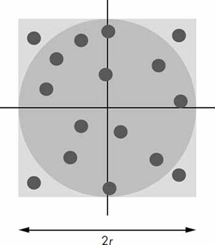
Figure 5-6: A circle of radius r inscribed in a square board with side 2r. The dots represent darts randomly thrown at the board.

As part of this challenge, write a program that will find the estimated area of a circle, given any radius, using this approach. The program should print the estimated area of the circle for three different values of the number of darts: 10³, 10⁵, and 10⁶. That’s a lot of darts! You’ll see that increasing the number of darts brings the estimated area close to the actual area. Here’s a sample output of the completed solution:

Radius: 2
Area: 12.566370614359172, Estimated (1000 darts): 12.576
Area: 12.566370614359172, Estimated (100000 darts): 12.58176
Area: 12.566370614359172, Estimated (1000000 darts): 12.560128

The dart throw can be simulated by a call to the random.uniform(a, b) function, which will return a random number between a and b. In this case, use the values a = 0, b = 2r (the side of the square).

Estimating the Value of Pi

Consider Figure 5-6 once again. The area of the square is 4r², and the area of the inscribed circle is πr². If we divide the area of the circle by the area of the square, we get π/4. The fraction f that we calculated earlier,

is thus an approximation of π/4, which in turn means that the value of

should be close to the value of π. Your next challenge is to write a program that will estimate the value of π assuming any value for the radius. As you increase the number of darts, the estimated value of π should get close to the known value of the constant.