Working with Data - Data Science from Scratch: First Principles with Python (2015)

Data Science from Scratch: First Principles with Python (2015)

Chapter 10. Working with Data

Experts often possess more data than judgment.

Colin Powell

Working with data is both an art and a science. We’ve mostly been talking about the science part, but in this chapter we’ll look at some of the art.

Exploring Your Data

After you’ve identified the questions you’re trying to answer and have gotten your hands on some data, you might be tempted to dive in and immediately start building models and getting answers. But you should resist this urge. Your first step should be to explore your data.

Exploring One-Dimensional Data

The simplest case is when you have a one-dimensional data set, which is just a collection of numbers. For example, these could be the daily average number of minutes each user spends on your site, the number of times each of a collection of data science tutorial videos was watched, or the number of pages of each of the data science books in your data science library.

An obvious first step is to compute a few summary statistics. You’d like to know how many data points you have, the smallest, the largest, the mean, and the standard deviation.

But even these don’t necessarily give you a great understanding. A good next step is to create a histogram, in which you group your data into discrete buckets and count how many points fall into each bucket:

def bucketize(point, bucket_size):
    """floor the point to the next lower multiple of bucket_size"""
    return bucket_size * math.floor(point / bucket_size)
 
def make_histogram(points, bucket_size):
    """buckets the points and counts how many in each bucket"""
    return Counter(bucketize(point, bucket_size) for point in points)
 
def plot_histogram(points, bucket_size, title=""):
    histogram = make_histogram(points, bucket_size)
    plt.bar(histogram.keys(), histogram.values(), width=bucket_size)
    plt.title(title)
    plt.show()

For example, consider the two following sets of data:

random.seed(0)
 
# uniform between -100 and 100
uniform = [200 * random.random() - 100 for _ in range(10000)]
 
# normal distribution with mean 0, standard deviation 57
normal = [57 * inverse_normal_cdf(random.random())
          for _ in range(10000)]

Both have means close to 0 and standard deviations close to 58. However, they have very different distributions. Figure 10-1 shows the distribution of uniform:

plot_histogram(uniform, 10, "Uniform Histogram")

while Figure 10-2 shows the distribution of normal:

plot_histogram(normal, 10, "Normal Histogram")

In this case, both distributions had pretty different max and min, but even knowing that wouldn’t have been sufficient to understand how they differed.

Histogram of uniform

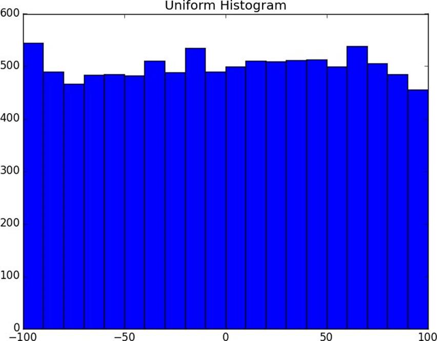
Figure 10-1. Histogram of uniform

Two Dimensions

Now imagine you have a data set with two dimensions. Maybe in addition to daily minutes you have years of data science experience. Of course you’d want to understand each dimension individually. But you probably also want to scatter the data.

For example, consider another fake data set:

def random_normal():
    """returns a random draw from a standard normal distribution"""
    return inverse_normal_cdf(random.random())
 
xs = [random_normal() for _ in range(1000)]
ys1 = [ x + random_normal() / 2 for x in xs]
ys2 = [-x + random_normal() / 2 for x in xs]

If you were to run plot_histogram on ys1 and ys2 you’d get very similar looking plots (indeed, both are normally distributed with the same mean and standard deviation).

Histogram of normal

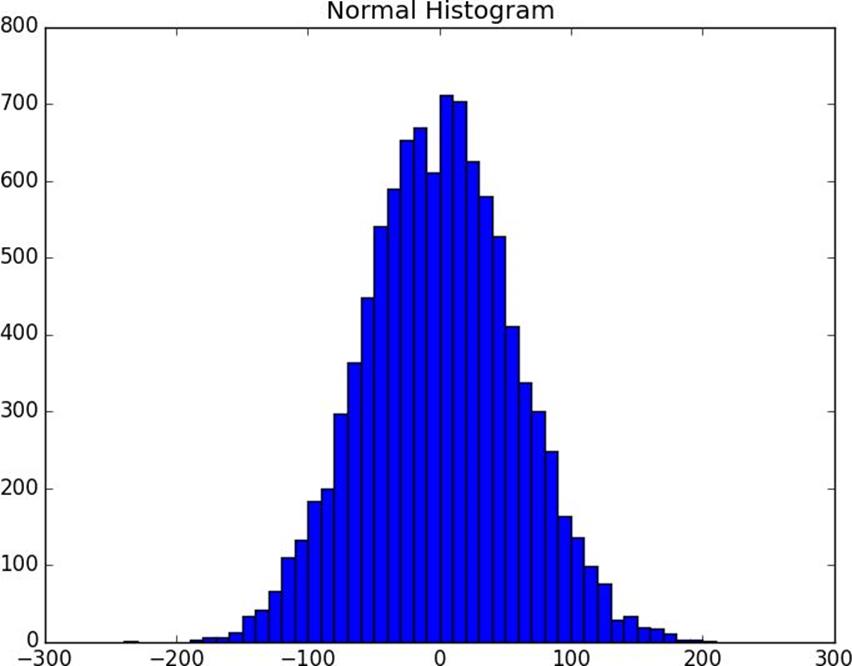
Figure 10-2. Histogram of normal

But each has a very different joint distribution with xs, as shown in Figure 10-3:

plt.scatter(xs, ys1, marker='.', color='black', label='ys1')
plt.scatter(xs, ys2, marker='.', color='gray',  label='ys2')
plt.xlabel('xs')
plt.ylabel('ys')
plt.legend(loc=9)
plt.title("Very Different Joint Distributions")
plt.show()

Scattering two different ys

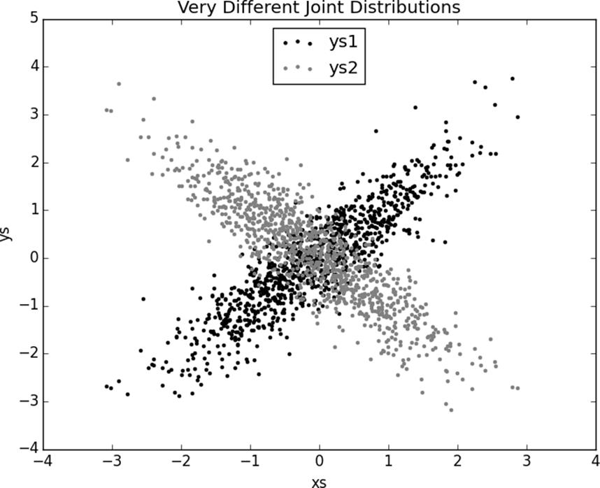
Figure 10-3. Scattering two different ys

This difference would also be apparent if you looked at the correlations:

print correlation(xs, ys1)      #  0.9
print correlation(xs, ys2)      # -0.9

Many Dimensions

With many dimensions, you’d like to know how all the dimensions relate to one another. A simple approach is to look at the correlation matrix, in which the entry in row i and column j is the correlation between the ith dimension and the jth dimension of the data:

def correlation_matrix(data):
    """returns the num_columns x num_columns matrix whose (i, j)th entry
    is the correlation between columns i and j of data"""
 
    _, num_columns = shape(data)
 
    def matrix_entry(i, j):
        return correlation(get_column(data, i), get_column(data, j))
 
    return make_matrix(num_columns, num_columns, matrix_entry)

A more visual approach (if you don’t have too many dimensions) is to make a scatterplot matrix (Figure 10-4) showing all the pairwise scatterplots. To do that we’ll use plt.subplots(), which allows us to create subplots of our chart. We give it the number of rows and the number of columns, and it returns a figure object (which we won’t use) and a two-dimensional array of axes objects (each of which we’ll plot to):

import matplotlib.pyplot as plt
 
_, num_columns = shape(data)
fig, ax = plt.subplots(num_columns, num_columns)
 
for i in range(num_columns):
    for j in range(num_columns):
 
        # scatter column_j on the x-axis vs column_i on the y-axis
        if i != j: ax[i][j].scatter(get_column(data, j), get_column(data, i))
 
        # unless i == j, in which case show the series name
        else: ax[i][j].annotate("series " + str(i), (0.5, 0.5),
                                xycoords='axes fraction',
                                ha="center", va="center")
 
        # then hide axis labels except left and bottom charts
        if i < num_columns - 1: ax[i][j].xaxis.set_visible(False)
        if j > 0: ax[i][j].yaxis.set_visible(False)
 
# fix the bottom right and top left axis labels, which are wrong because
# their charts only have text in them
ax[-1][-1].set_xlim(ax[0][-1].get_xlim())
ax[0][0].set_ylim(ax[0][1].get_ylim())
 
plt.show()

Scatterplot matrix

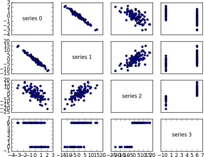
Figure 10-4. Scatterplot matrix

Looking at the scatterplots, you can see that series 1 is very negatively correlated with series 0, series 2 is positively correlated with series 1, and series 3 only takes on the values 0 and 6, with 0 corresponding to small values of series 2 and 6 corresponding to large values.

This is a quick way to get a rough sense of which of your variables are correlated (unless you spend hours tweaking matplotlib to display things exactly the way you want them to, in which case it’s not a quick way).

Cleaning and Munging

Real-world data is dirty. Often you’ll have to do some work on it before you can use it. We’ve seen examples of this in Chapter 9. We have to convert strings to floats or ints before we can use them. Previously, we did that right before using the data:

        closing_price = float(row[2])

But it’s probably less error-prone to do the parsing on the way in, which we can do by creating a function that wraps csv.reader. We’ll give it a list of parsers, each specifying how to parse one of the columns. And we’ll use None to represent “don’t do anything to this column”:

def parse_row(input_row, parsers):
    """given a list of parsers (some of which may be None)
    apply the appropriate one to each element of the input_row"""
 
    return [parser(value) if parser is not None else value
            for value, parser in zip(input_row, parsers)]
 
def parse_rows_with(reader, parsers):
    """wrap a reader to apply the parsers to each of its rows"""
    for row in reader:
        yield parse_row(row, parsers)

What if there’s bad data? A “float” value that doesn’t actually represent a number? We’d usually rather get a None than crash our program. We can do this with a helper function:

def try_or_none(f):
    """wraps f to return None if f raises an exception
    assumes f takes only one input"""
    def f_or_none(x):
        try: return f(x)
        except: return None
    return f_or_none

after which we can rewrite parse_row to use it:

def parse_row(input_row, parsers):
    return [try_or_none(parser)(value) if parser is not None else value
            for value, parser in zip(input_row, parsers)]

For example, if we have comma-delimited stock prices with bad data:

6/20/2014,AAPL,90.91
6/20/2014,MSFT,41.68
6/20/3014,FB,64.5
6/19/2014,AAPL,91.86
6/19/2014,MSFT,n/a
6/19/2014,FB,64.34

we can now read and parse in a single step:

import dateutil.parser
data = []
 
with open("comma_delimited_stock_prices.csv", "rb") as f:
    reader = csv.reader(f)
    for line in parse_rows_with(reader, [dateutil.parser.parse, None, float]):
        data.append(line)

after which we just need to check for None rows:

for row in data:
    if any(x is None for x in row):
        print row

and decide what we want to do about them. (Generally speaking, the three options are to get rid of them, to go back to the source and try to fix the bad/missing data, or to do nothing and cross our fingers.)

We could create similar helpers for csv.DictReader. In that case, you’d probably want to supply a dict of parsers by field name. For example:

def try_parse_field(field_name, value, parser_dict):
    """try to parse value using the appropriate function from parser_dict"""
    parser = parser_dict.get(field_name)   # None if no such entry
    if parser is not None:
        return try_or_none(parser)(value)
    else:
        return value
 
def parse_dict(input_dict, parser_dict):
    return { field_name : try_parse_field(field_name, value, parser_dict)
             for field_name, value in input_dict.iteritems() }

A good next step is to check for outliers, using techniques from “Exploring Your Data” or by ad hoc investigating. For example, did you notice that one of the dates in the stocks file had the year 3014? That won’t (necessarily) give you an error, but it’s quite plainly wrong, and you’ll get screwy results if you don’t catch it. Real-world data sets have missing decimal points, extra zeroes, typographical errors, and countless other problems that it’s your job to catch. (Maybe it’s not officially your job, but who else is going to do it?)

Manipulating Data

One of the most important skills of a data scientist is manipulating data. It’s more of a general approach than a specific technique, so we’ll just work through a handful of examples to give you the flavor of it.

Imagine we’re working with dicts of stock prices that look like:

data = [
    {'closing_price': 102.06,
     'date': datetime.datetime(2014, 8, 29, 0, 0),
     'symbol': 'AAPL'},
    # ...
]

Conceptually we’ll think of them as rows (as in a spreadsheet).

Let’s start asking questions about this data. Along the way we’ll try to notice patterns in what we’re doing and abstract out some tools to make the manipulation easier.

For instance, suppose we want to know the highest-ever closing price for AAPL. Let’s break this down into concrete steps:

1. Restrict ourselves to AAPL rows.

2. Grab the closing_price from each row.

3. Take the max of those prices.

We can do all three at once using a list comprehension:

max_aapl_price = max(row["closing_price"]
                     for row in data
                     if row["symbol"] == "AAPL")

More generally, we might want to know the highest-ever closing price for each stock in our data set. One way to do this is:

1. Group together all the rows with the same symbol.

2. Within each group, do the same as before:

# group rows by symbol
by_symbol = defaultdict(list)
for row in data:
    by_symbol[row["symbol"]].append(row)
 
# use a dict comprehension to find the max for each symbol
max_price_by_symbol = { symbol : max(row["closing_price"]
                                     for row in grouped_rows)
                        for symbol, grouped_rows in by_symbol.iteritems() }

There are some patterns here already. In both examples, we needed to pull the closing_price value out of every dict. So let’s create a function to pick a field out of a dict, and another function to pluck the same field out of a collection of dicts:

def picker(field_name):
    """returns a function that picks a field out of a dict"""
    return lambda row: row[field_name]
 
def pluck(field_name, rows):
    """turn a list of dicts into the list of field_name values"""
    return map(picker(field_name), rows)

We can also create a function to group rows by the result of a grouper function and to optionally apply some sort of value_transform to each group:

def group_by(grouper, rows, value_transform=None):
    # key is output of grouper, value is list of rows
    grouped = defaultdict(list)
    for row in rows:
        grouped[grouper(row)].append(row)
 
    if value_transform is None:
        return grouped
    else:
        return { key : value_transform(rows)
                 for key, rows in grouped.iteritems() }

This allows us to rewrite our previous examples quite simply. For example:

max_price_by_symbol = group_by(picker("symbol"),
                               data,
                               lambda rows: max(pluck("closing_price", rows)))

We can now start to ask more complicated things, like what are the largest and smallest one-day percent changes in our data set. The percent change is price_today / price_yesterday - 1, which means we need some way of associating today’s price and yesterday’s price. One approach is to group the prices by symbol, then, within each group:

1. Order the prices by date.

2. Use zip to get pairs (previous, current).

3. Turn the pairs into new “percent change” rows.

We’ll start by writing a function to do all the within-each-group work:

def percent_price_change(yesterday, today):
    return today["closing_price"] / yesterday["closing_price"] - 1
 
def day_over_day_changes(grouped_rows):
    # sort the rows by date
    ordered = sorted(grouped_rows, key=picker("date"))
 
    # zip with an offset to get pairs of consecutive days
    return [{ "symbol" : today["symbol"],
              "date" : today["date"],
              "change" : percent_price_change(yesterday, today) }
            for yesterday, today in zip(ordered, ordered[1:])]

Then we can just use this as the value_transform in a group_by:

# key is symbol, value is list of "change" dicts
changes_by_symbol = group_by(picker("symbol"), data, day_over_day_changes)
 
# collect all "change" dicts into one big list
all_changes = [change
               for changes in changes_by_symbol.values()
               for change in changes]

At which point it’s easy to find the largest and smallest:

max(all_changes, key=picker("change"))
# {'change': 0.3283582089552237,
#  'date': datetime.datetime(1997, 8, 6, 0, 0),
#  'symbol': 'AAPL'}
# see, e.g. http://news.cnet.com/2100-1001-202143.html
 
min(all_changes, key=picker("change"))
# {'change': -0.5193370165745856,
#  'date': datetime.datetime(2000, 9, 29, 0, 0),
#  'symbol': 'AAPL'}
# see, e.g. http://money.cnn.com/2000/09/29/markets/techwrap/

We can now use this new all_changes data set to find which month is the best to invest in tech stocks. First we group the changes by month; then we compute the overall change within each group.

Once again, we write an appropriate value_transform and then use group_by:

# to combine percent changes, we add 1 to each, multiply them, and subtract 1
# for instance, if we combine +10% and -20%, the overall change is
#    (1 + 10%) * (1 - 20%) - 1 = 1.1 * .8 - 1 = -12%
def combine_pct_changes(pct_change1, pct_change2):
    return (1 + pct_change1) * (1 + pct_change2) - 1
 
def overall_change(changes):
    return reduce(combine_pct_changes, pluck("change", changes))
 
overall_change_by_month = group_by(lambda row: row['date'].month,
                                   all_changes,
                                   overall_change)

We’ll be doing these sorts of manipulations throughout the book, usually without calling too much explicit attention to them.

Rescaling

Many techniques are sensitive to the scale of your data. For example, imagine that you have a data set consisting of the heights and weights of hundreds of data scientists, and that you are trying to identify clusters of body sizes.

Intuitively, we’d like clusters to represent points near each other, which means that we need some notion of distance between points. We already have a Euclidean distance function, so a natural approach might be to treat (height, weight) pairs as points in two-dimensional space. Consider the people listed in Table 10-1.

Person

Height (inches)

Height (centimeters)

Weight

A

63 inches

160 cm

150 pounds

B

67 inches

170.2 cm

160 pounds

C

70 inches

177.8 cm

171 pounds

Table 10-1. Heights and Weights

If we measure height in inches, then B’s nearest neighbor is A:

a_to_b = distance([63, 150], [67, 160])        # 10.77
a_to_c = distance([63, 150], [70, 171])        # 22.14
b_to_c = distance([67, 160], [70, 171])        # 11.40

However, if we measure height in centimeters, then B’s nearest neighbor is instead C:

a_to_b = distance([160, 150], [170.2, 160])    # 14.28
a_to_c = distance([160, 150], [177.8, 171])    # 27.53
b_to_c = distance([170.2, 160], [177.8, 171])  # 13.37

Obviously it’s problematic if changing units can change results like this. For this reason, when dimensions aren’t comparable with one another, we will sometimes rescale our data so that each dimension has mean 0 and standard deviation 1. This effectively gets rid of the units, converting each dimension to “standard deviations from the mean.”

To start with, we’ll need to compute the mean and the standard_deviation for each column:

def scale(data_matrix):
    """returns the means and standard deviations of each column"""
    num_rows, num_cols = shape(data_matrix)
    means = [mean(get_column(data_matrix,j))
             for j in range(num_cols)]
    stdevs = [standard_deviation(get_column(data_matrix,j))
              for j in range(num_cols)]
    return means, stdevs

And then use them to create a new data matrix:

def rescale(data_matrix):
    """rescales the input data so that each column
    has mean 0 and standard deviation 1
    leaves alone columns with no deviation"""
    means, stdevs = scale(data_matrix)
 
    def rescaled(i, j):
        if stdevs[j] > 0:
            return (data_matrix[i][j] - means[j]) / stdevs[j]
        else:
            return data_matrix[i][j]
 
    num_rows, num_cols = shape(data_matrix)
    return make_matrix(num_rows, num_cols, rescaled)

As always, you need to use your judgment. If you were to take a huge data set of heights and weights and filter it down to only the people with heights between 69.5 inches and 70.5 inches, it’s quite likely (depending on the question you’re trying to answer) that the variation remaining is simply noise, and you might not want to put its standard deviation on equal footing with other dimensions’ deviations.

Dimensionality Reduction

Sometimes the “actual” (or useful) dimensions of the data might not correspond to the dimensions we have. For example, consider the data set pictured in Figure 10-5.

Data with the 'wrong' axes

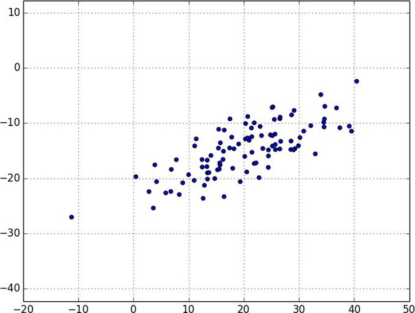
Figure 10-5. Data with the “wrong” axes

Most of the variation in the data seems to be along a single dimension that doesn’t correspond to either the x-axis or the y-axis.

When this is the case, we can use a technique called principal component analysis to extract one or more dimensions that capture as much of the variation in the data as possible.

NOTE

In practice, you wouldn’t use this technique on such a low-dimensional data set. Dimensionality reduction is mostly useful when your data set has a large number of dimensions and you want to find a small subset that captures most of the variation. Unfortunately, that case is difficult to illustrate in a two-dimensional book format.

As a first step, we’ll need to translate the data so that each dimension has mean zero:

def de_mean_matrix(A):
    """returns the result of subtracting from every value in A the mean
    value of its column. the resulting matrix has mean 0 in every column"""
    nr, nc = shape(A)
    column_means, _ = scale(A)
    return make_matrix(nr, nc, lambda i, j: A[i][j] - column_means[j])

(If we don’t do this, our techniques are likely to identify the mean itself rather than the variation in the data.)

Figure 10-6 shows the example data after de-meaning.

PCA data with mean removed.

Figure 10-6. Data after de-meaning

Now, given a de-meaned matrix X, we can ask which is the direction that captures the greatest variance in the data?

Specifically, given a direction d (a vector of magnitude 1), each row x in the matrix extends dot(x, d) in the d direction. And every nonzero vector w determines a direction if we rescale it to have magnitude 1:

def direction(w):
    mag = magnitude(w)
    return [w_i / mag for w_i in w]

Therefore, given a nonzero vector w, we can compute the variance of our data set in the direction determined by w:

def directional_variance_i(x_i, w):
    """the variance of the row x_i in the direction determined by w"""
    return dot(x_i, direction(w)) ** 2
 
def directional_variance(X, w):
    """the variance of the data in the direction determined w"""
    return sum(directional_variance_i(x_i, w)
               for x_i in X)

We’d like to find the direction that maximizes this variance. We can do this using gradient descent, as soon as we have the gradient function:

def directional_variance_gradient_i(x_i, w):
    """the contribution of row x_i to the gradient of
    the direction-w variance"""
    projection_length = dot(x_i, direction(w))
    return [2 * projection_length * x_ij for x_ij in x_i]
 
def directional_variance_gradient(X, w):
    return vector_sum(directional_variance_gradient_i(x_i,w)
                      for x_i in X)

The first principal component is just the direction that maximizes the directional_variance function:

def first_principal_component(X):
    guess = [1 for _ in X[0]]
    unscaled_maximizer = maximize_batch(
        partial(directional_variance, X),           # is now a function of w
        partial(directional_variance_gradient, X),  # is now a function of w
        guess)
    return direction(unscaled_maximizer)

Or, if you’d rather use stochastic gradient descent:

# here there is no "y", so we just pass in a vector of Nones
# and functions that ignore that input
def first_principal_component_sgd(X):
    guess = [1 for _ in X[0]]
    unscaled_maximizer = maximize_stochastic(
        lambda x, _, w: directional_variance_i(x, w),
        lambda x, _, w: directional_variance_gradient_i(x, w),
        X,
        [None for _ in X],   # the fake "y"
        guess)
    return direction(unscaled_maximizer)

On the de-meaned data set, this returns the direction [0.924, 0.383], which does appear to capture the primary axis along which our data varies (Figure 10-7).

PCA data with first component.

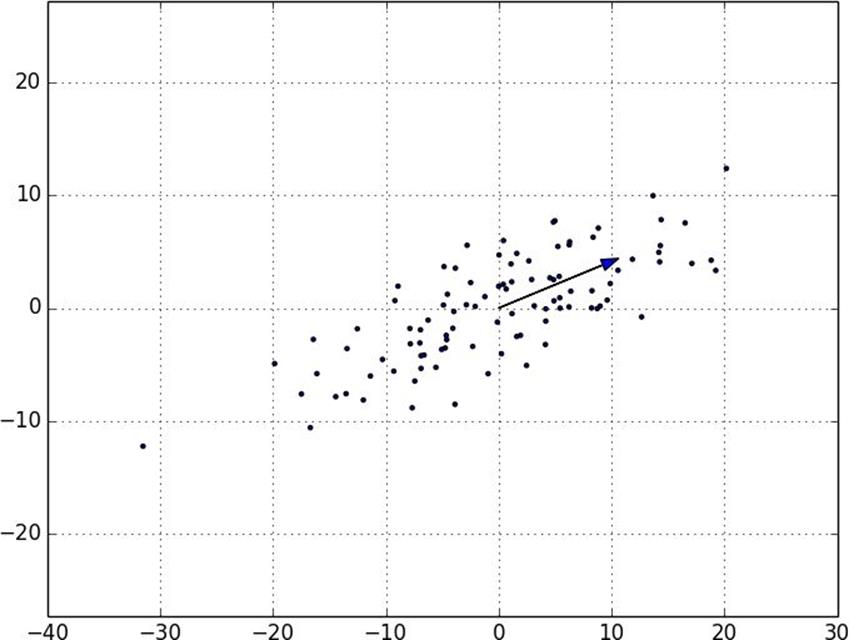
Figure 10-7. First principal component

Once we’ve found the direction that’s the first principal component, we can project our data onto it to find the values of that component:

def project(v, w):
    """return the projection of v onto the direction w"""
    projection_length = dot(v, w)
    return scalar_multiply(projection_length, w)

If we want to find further components, we first remove the projections from the data:

def remove_projection_from_vector(v, w):
    """projects v onto w and subtracts the result from v"""
    return vector_subtract(v, project(v, w))
 
def remove_projection(X, w):
    """for each row of X
    projects the row onto w, and subtracts the result from the row"""
    return [remove_projection_from_vector(x_i, w) for x_i in X]

Because this example data set is only two-dimensional, after we remove the first component, what’s left will be effectively one-dimensional (Figure 10-8).

Data after removing first principal component

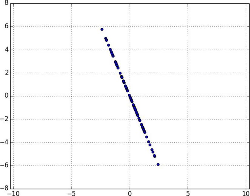
Figure 10-8. Data after removing first principal component

At that point, we can find the next principal component by repeating the process on the result of remove_projection (Figure 10-9).

On a higher-dimensional data set, we can iteratively find as many components as we want:

def principal_component_analysis(X, num_components):
    components = []
    for _ in range(num_components):
        component = first_principal_component(X)
        components.append(component)
        X = remove_projection(X, component)
 
    return components

We can then transform our data into the lower-dimensional space spanned by the components:

def transform_vector(v, components):
    return [dot(v, w) for w in components]
 
def transform(X, components):
    return [transform_vector(x_i, components) for x_i in X]

This technique is valuable for a couple of reasons. First, it can help us clean our data by eliminating noise dimensions and consolidating dimensions that are highly correlated.

First two principal components.

Figure 10-9. First two principal components

Second, after extracting a low-dimensional representation of our data, we can use a variety of techniques that don’t work as well on high-dimensional data. We’ll see examples of such techniques throughout the book.

At the same time, while it can help you build better models, it can also make those models harder to interpret. It’s easy to understand conclusions like “every extra year of experience adds an average of $10k in salary.” It’s much harder to make sense of “every increase of 0.1 in the third principal component adds an average of $10k in salary.”

For Further Exploration

§ As we mentioned at the end of Chapter 9, pandas is probably the primary Python tool for cleaning, munging, manipulating, and working with data. All the examples we did by hand in this chapter could be done much more simply using pandas. Python for Data Analysis (O’Reilly) is probably the best way to learn pandas.

§ scikit-learn has a wide variety of matrix decomposition functions, including PCA.