Machine Learning - Data Science from Scratch: First Principles with Python (2015)
Data Science from Scratch: First Principles with Python (2015)
Chapter 11.Machine Learning
I am always ready to learn although I do not always like being taught.
Winston Churchill
Many people imagine that data science ismostly machine learning and that data scientists mostly build and train and tweak machine-learning models all day long. (Then again, many of those people don’t actually know what machine learningis.) In fact, data science is mostly turning business problems into data problems and collecting data and understanding data and cleaning data and formatting data, after which machine learning is almost an afterthought. Even so, it’s an interesting and essential afterthought that you pretty much have to know about in order to do data science.
Modeling
Before we can talk about machine learning we need totalk aboutmodels.
What is a model? It’s simply a specification of a mathematical (or probabilistic) relationship that exists between different variables.
For instance, if you’re trying to raise money for your social networking site, you mightbuild abusiness model(likely in a spreadsheet) that takes inputs like “number of users” and “ad revenue per user” and “number of employees” and outputs your annual profit for the next several years. A cookbook recipe entails a model that relates inputs like “number of eaters” and “hungriness” to quantities of ingredients needed. And if you’ve ever watched poker on television, you know that they estimate each player’s “win probability” in real time based on a model that takes into account the cards that have been revealed so far and the distribution of cards in the deck.
The business model is probably based on simple mathematical relationships: profit is revenue minus expenses, revenue is units sold times average price, and so on. The recipe model is probably based on trial and error — someone went in a kitchen and tried different combinations of ingredients until they found one they liked. And the poker model is based on probability theory, the rules of poker, and some reasonably innocuous assumptions about the random process by which cards are dealt.
What Is Machine Learning?
Everyone has her own exact definition, but we’ll usemachine learningto refer to creating and usingmodels that arelearned from data.In other contexts this might be calledpredictive modelingordata mining, but we will stick with machine learning. Typically, our goal will be to use existing data to develop models that we can use topredictvarious outcomes for new data, such as:
§ Predicting whether an email message is spam or not
§ Predicting whether a credit card transaction is fraudulent
§ Predicting which advertisement a shopper is most likely to click on
§ Predicting which football team is going to win the Super Bowl
We’ll look atbothsupervisedmodels (in which there is a set of data labeled with the correct answers to learn from), andunsupervisedmodels (in which there are no such labels).There are various other types likesemisupervised(in which only some of the data are labeled) andonline(in which the model needs to continuously adjust to newly arriving data) that we won’t cover in this book.
Now, in even the simplest situation there are entire universes of models that might describe the relationship we’re interested in. In most cases we will ourselves choose aparameterizedfamily of modelsand then use data to learn parameters that are in some way optimal.
For instance, we might assume that a person’s height is (roughly) a linear function of his weight and then use data to learn what that linear function is. Or we might assume that a decision tree is a good way to diagnose what diseases our patients have and then use data to learn the “optimal” such tree. Throughout the rest of the book we’ll be investigating different families of models that we can learn.
But before we can do that, we need to better understand the fundamentals of machine learning. For the rest of the chapter, we’ll discuss some of those basic concepts, before we move on to the models themselves.
Overfitting and Underfitting
A common danger in machine learning isoverfitting— producing a model that performs well on the data you trainit on but that generalizes poorly to any new data.This could involve learningnoisein the data. Or it could involve learning to identify specific inputs rather than whatever factors are actually predictive for the desired output.
The other side ofthis isunderfitting, producing a model that doesn’t perform well even on the training data, although typically when this happens you decide your model isn’t good enough and keep looking for a better one.
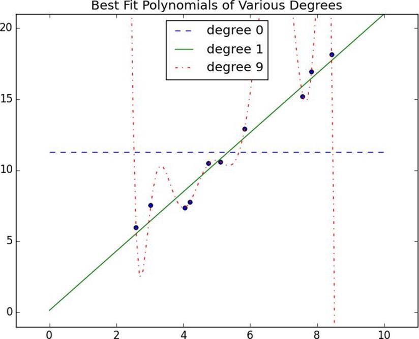
Figure 11-1.Overfitting and underfitting
InFigure 11-1, I’ve fit three polynomials to a sample of data. (Don’t worry about how; we’ll get to that in later chapters.)
The horizontal line shows the best fit degree 0 (i.e., constant) polynomial. It severelyunderfitsthe training data. The best fit degree 9 (i.e., 10-parameter) polynomial goes through every training data point exactly, but it very severelyoverfits— if we were to pick a few more data points it would quite likely miss them by a lot. And the degree 1 line strikes a nice balance — it’s pretty close to every point, and (if these data are representative) the line will likely be close to new data points as well.
Clearly models that are too complex lead to overfitting and don’t generalize well beyond the data they were trained on. So how do we make sure our models aren’t too complex? The most fundamental approach involves using different data to train the model and to test the model.
The simplest way to do this is to split your data set, so that (for example) two-thirds of it is used to train the model, after which we measure the model’s performance on the remaining third:
defsplit_data(data,prob):
"""split data into fractions [prob, 1 - prob]"""
results=[],[]
forrowindata:
results[0ifrandom.random()<probelse1].append(row)
returnresults
Often, we’ll have a matrixxof input variables and a vectoryof output variables. In that case, we need to make sure to put corresponding values together in either the training data or the test data:
deftrain_test_split(x,y,test_pct):
data=zip(x,y)# pair corresponding values
train,test=split_data(data,1-test_pct)# split the data set of pairs
If the model was overfit to the training data, then it will hopefully perform really poorly on the (completely separate) test data. Said differently, if it performs well on the test data, then you can be more confident that it’sfittingrather thanoverfitting.
However, there are a couple of ways this can go wrong.
The first is if there are common patterns in the test and train data that wouldn’t generalize to a larger data set.
For example, imagine that your data set consists of user activity, one row per user per week. In such a case, most users will appear in both the training data and the test data, and certain models might learn toidentifyusers rather than discover relationships involvingattributes. This isn’t a huge worry, although it did happen to me once.
A bigger problem is if you use the test/train split not just to judge a model but also tochoosefrom among many models. In that case, although each individual model may not be overfit, the “choose a model that performs best on the test set” is a meta-training that makes the test set function as a second training set. (Of course the model that performed best on the test set is going to perform well on the test set.)
In such a situation, you should split the data into three parts: atrainingset for building models, avalidationset for choosing among trained models, and atestset for judging the final model.
Correctness
When I’m not doing data science, I dabble in medicine.And in my spare time I’ve come up with a cheap, noninvasive test that can be given to a newborn baby that predicts — with greater than 98% accuracy — whether the newborn will ever develop leukemia. My lawyer has convinced me the test is unpatentable, so I’ll share with you the details here: predict leukemia if and only if the baby is named Luke (which sounds sort of like “leukemia”).
As we’ll see below, this test is indeed more than 98% accurate. Nonetheless, it’s an incredibly stupid test, and a good illustration of why we don’t typically use “accuracy” to measure how good a model is.
Imagine building a model to make abinaryjudgment. Is this email spam? Should we hire this candidate? Is this air traveler secretly a terrorist?
Given a set of labeled data and such a predictive model, every data point lies in one of four categories:
§ True positive: “This message is spam, and we correctly predicted spam.”
§ False positive (Type 1 Error): “This message is not spam, but we predicted spam.”
§ False negative (Type 2 Error): “This message is spam, but we predicted not spam.”
§ True negative: “This message is not spam, and we correctly predicted not spam.”
We often represent these as countsin aconfusion matrix:
Spam
not Spam
predict “Spam”
True Positive
False Positive
predict “Not Spam”
False Negative
True Negative
Let’s see how my leukemia test fits into this framework. These days approximately5 babies out of 1,000 are named Luke. And the lifetime prevalence of leukemia is about 1.4%, or14 out of every 1,000 people.
If we believe these two factors are independent and apply my “Luke is for leukemia” test to 1 million people, we’d expect to see a confusion matrix like:
leukemia
no leukemia
total
“Luke”
70
4,930
5,000
not “Luke”
13,930
981,070
995,000
total
14,000
986,000
1,000,000
We can then use these to compute various statistics about model performance. For example,accuracyisdefined as the fraction of correct predictions:
defaccuracy(tp,fp,fn,tn):
correct=tp+tn
total=tp+fp+fn+tn
returncorrect/total
printaccuracy(70,4930,13930,981070)# 0.98114
That seems like a pretty impressive number. But clearly this is not a good test, which means that we probably shouldn’t put a lot of credence in raw accuracy.
It’s common to look at the combination ofprecisionandrecall.Precision measures how accurate ourpositivepredictions were:
defprecision(tp,fp,fn,tn):
returntp/(tp+fp)
printprecision(70,4930,13930,981070)# 0.014
And recall measures whatfraction of the positives our model identified:
defrecall(tp,fp,fn,tn):
returntp/(tp+fn)
printrecall(70,4930,13930,981070)# 0.005
These are both terrible numbers, reflecting that this is a terrible model.
Sometimes precision and recall arecombined into theF1 score, which is defined as:
deff1_score(tp,fp,fn,tn):
p=precision(tp,fp,fn,tn)
r=recall(tp,fp,fn,tn)
return2*p*r/(p+r)
This is theharmonic meanof precisionand recall and necessarily lies between them.
Usually the choice of a model involves a trade-off between precision and recall. A model that predicts “yes” when it’s even a little bit confident will probably have a high recall but a low precision; a model that predicts “yes” only when it’s extremely confident is likely to have a low recall and a high precision.
Alternatively, you can think of this as a trade-off between false positives and false negatives. Saying “yes” too often will give you lots of false positives; saying “no” too often will give you lots of false negatives.
Imagine that there were 10 risk factors for leukemia, and that the more of them you had the more likely you were to develop leukemia. In that case you can imagine a continuum of tests: “predict leukemia if at least one risk factor,” “predict leukemia if at least two risk factors,” and so on. As you increase the threshhold, you increase the test’s precision (since people with more risk factors are more likely to develop the disease), and you decrease the test’s recall (since fewer and fewer of the eventual disease-sufferers will meet the threshhold). In cases like this, choosing the right threshhold is a matter of finding the right trade-off.
The Bias-Variance Trade-off
Another way of thinking about the overfitting problem is as a trade-off between bias and variance.
Both are measures of what would happen if you were to retrain your model many times on different sets of training data (from the same larger population).
For example, the degree 0 model in“Overfitting and Underfitting”will make a lot of mistakes for pretty much any training set (drawn from the same population), which means that it has a highbias.However, any two randomly chosen training sets should give pretty similar models (since any two randomly chosen training sets should have pretty similar average values). So we say that it has a lowvariance.High bias and low variance typically correspond to underfitting.
On the other hand, the degree 9 model fit the training set perfectly. It has very low bias but very high variance (since any two training sets would likely give rise to very different models).This corresponds to overfitting.
Thinking about model problems this way can help you figure out what do when your model doesn’t work so well.
If your model has high bias (which means it performs poorly even on your training data) then one thing to try is adding more features. Going from the degree 0 model in“Overfitting and Underfitting”to the degree 1 model was a big improvement.
If your model has high variance, then you can similarlyremovefeatures.But another solution is to obtain more data (if you can).
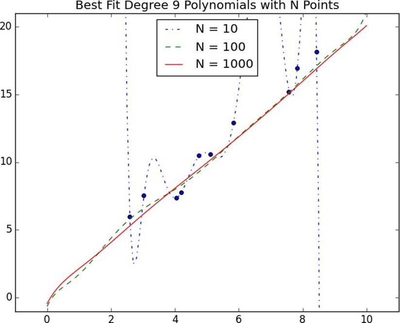
Figure 11-2.Reducing variance with more data
InFigure 11-2, we fit a degree 9 polynomial to different size samples. The model fit based on 10 data points is all over the place, as we saw before. If we instead trained on 100 data points, there’s much less overfitting. And the model trained from 1,000 data points looks very similar to the degree 1 model.
Holding model complexity constant, the more data you have, the harder it is to overfit.
On the other hand, more data won’t help with bias.If your model doesn’t use enough features to capture regularities in the data, throwing more data at it won’t help.
Feature Extraction and Selection
As we mentioned, when your data doesn’t have enough features, your model is likely to underfit.And when your data has too many features, it’s easy to overfit. But what are features and where do they come from?
Featuresare whatever inputswe provide to our model.
In the simplest case, features are simply given to you. If you want to predict someone’s salary based on her years of experience, then years of experience is the only feature you have.
(Although, as we saw in“Overfitting and Underfitting”, you might also consider adding years of experience squared, cubed, and so on if that helps you build a better model.)
Things become more interesting as your data becomes more complicated. Imagine trying to build a spam filter to predict whether an email is junk or not. Most models won’t know what to do with a raw email, which is just a collection of text.You’ll have to extract features. For example:
§ Does the email contain the word “Viagra”?
§ How many times does the letter d appear?
§ What was the domain of the sender?
The first is simply a yes or no, which we typically encode as a 1 or 0. The second is a number. And the third is a choice from a discrete set of options.
Pretty much always, we’ll extract features from our data that fall into one of these three categories. What’s more, the type of features we have constrains the type of models we can use.
The Naive Bayes classifier we’ll build inChapter 13is suited to yes-or-no features, like the first one in the preceding list.
Regression models, as we’ll study inChapter 14andChapter 16, require numeric features (which could include dummy variables that are 0s and 1s).
And decision trees, which we’ll look at inChapter 17, can deal with numeric or categorical data.
Although in the spam filter example we looked for ways to create features, sometimes we’ll instead look for ways to remove features.
For example, your inputs might be vectors of several hundred numbers. Depending on the situation, it might be appropriate to distill these down to handful of important dimensions (as in“Dimensionality Reduction”) and use only those small number of features. Or it might be appropriate to use a technique (like regularization, which we’ll look at in“Regularization”) that penalizes models the more features they use.
How do we choosefeatures? That’s where a combination ofexperienceanddomain expertisecomes into play. If you’ve received lots of emails, then you probably have a sense that the presence of certain words might be a good indicator of spamminess. And you might also have a sense that the number of d’s is likely not a good indicator of spamminess. But in general you’ll have to try different things, which is part of the fun.
For Further Exploration
§ Keep reading! The next several chapters are about different families of machine-learning models.
§ The CourseraMachine Learningcourse is the original MOOC and is a good place to get a deeper understanding of the basics of machine learning. The CaltechMachine LearningMOOC is also good.
§ The Elements of Statistical Learningis a somewhat canonical textbook that can bedownloaded online for free. But be warned: it’sverymathy.