Data Science from Scratch: First Principles with Python (2015)
Chapter 14. Simple Linear Regression
Art, like morality, consists in drawing the line somewhere.
G. K. Chesterton
The Model
In particular, you hypothesize that there are constants ![]() (alpha) and
(alpha) and ![]() (beta) such that:
(beta) such that:
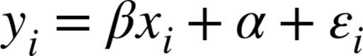
where ![]() is the number of minutes user i spends on the site daily,
is the number of minutes user i spends on the site daily, ![]() is the number of friends user i has, and
is the number of friends user i has, and ![]() is a (hopefully small) error term representing the fact that there are other factors not accounted for by this simple model.
is a (hopefully small) error term representing the fact that there are other factors not accounted for by this simple model.
defpredict(alpha,beta,x_i):
returnbeta*x_i+alpha
deferror(alpha,beta,x_i,y_i):
"""the error from predicting beta * x_i + alpha
when the actual value is y_i"""returny_i-predict(alpha,beta,x_i)
defsum_of_squared_errors(alpha,beta,x,y):
returnsum(error(alpha,beta,x_i,y_i)**2
forx_i,y_iinzip(x,y))
defleast_squares_fit(x,y):
"""given training values for x and y,
find the least-squares values of alpha and beta"""beta=correlation(x,y)*standard_deviation(y)/standard_deviation(x)
alpha=mean(y)-beta*mean(x)
returnalpha,beta
alpha,beta=least_squares_fit(num_friends_good,daily_minutes_good)
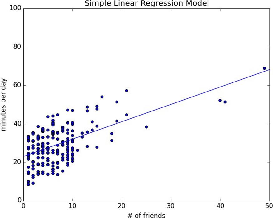
Figure 14-1. Our simple linear model
deftotal_sum_of_squares(y):
"""the total squared variation of y_i's from their mean"""
returnsum(v**2forvinde_mean(y))
defr_squared(alpha,beta,x,y):
"""the fraction of variation in y captured by the model, which equals
1 - the fraction of variation in y not captured by the model"""return1.0-(sum_of_squared_errors(alpha,beta,x,y)/
total_sum_of_squares(y))
r_squared(alpha,beta,num_friends_good,daily_minutes_good)# 0.329
Using Gradient Descent
defsquared_error(x_i,y_i,theta):
alpha,beta=theta
returnerror(alpha,beta,x_i,y_i)**2
defsquared_error_gradient(x_i,y_i,theta):
alpha,beta=theta
return[-2*error(alpha,beta,x_i,y_i),# alpha partial derivative
-2*error(alpha,beta,x_i,y_i)*x_i]# beta partial derivative
# choose random value to startrandom.seed(0)theta=[random.random(),random.random()]
alpha,beta=minimize_stochastic(squared_error,
squared_error_gradient,
num_friends_good,
daily_minutes_good,
theta,
0.0001)
alpha,beta
Maximum Likelihood Estimation
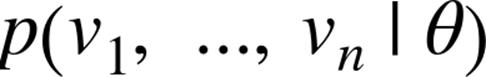
Imagine that we have a sample of data ![]() that comes from a distribution that depends on some unknown parameter
that comes from a distribution that depends on some unknown parameter ![]() :
:
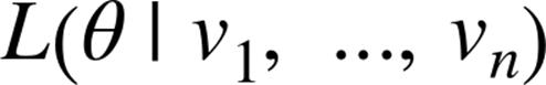
If we didn’t know theta, we could turn around and think of this quantity as the likelihood of ![]() given the sample:
given the sample:
Under this approach, the most likely ![]() is the value that maximizes this likelihood function; that is, the value that makes the observed data the most probable. In the case of a continuous distribution, in which we have a probability distribution function rather than a probability mass function, we can do the same thing.
is the value that maximizes this likelihood function; that is, the value that makes the observed data the most probable. In the case of a continuous distribution, in which we have a probability distribution function rather than a probability mass function, we can do the same thing.
Back to regression. One assumption that’s often made about the simple regression model is that the regression errors are normally distributed with mean 0 and some (known) standard deviation ![]() . If that’s the case, then the likelihood based on seeing a pair
. If that’s the case, then the likelihood based on seeing a pair (x_i, y_i) is:

For Further Exploration
All materials on the site are licensed Creative Commons Attribution-Sharealike 3.0 Unported CC BY-SA 3.0 & GNU Free Documentation License (GFDL)
If you are the copyright holder of any material contained on our site and intend to remove it, please contact our site administrator for approval.
© 2016-2026 All site design rights belong to S.Y.A.