Data Science from Scratch: First Principles with Python (2015)
Chapter 15. Multiple Regression
I don’t look at a problem and put variables in there that don’t affect it.
Bill Parcells

The Model

Now imagine that each input ![]() is not a single number but rather a vector of k numbers
is not a single number but rather a vector of k numbers ![]() . The multiple regression model assumes that:
. The multiple regression model assumes that:

In multiple regression the vector of parameters is usually called ![]() . We’ll want this to include the constant term as well, which we can achieve by adding a column of ones to our data:
. We’ll want this to include the constant term as well, which we can achieve by adding a column of ones to our data:
beta=[alpha,beta_1,...,beta_k]
x_i=[1,x_i1,...,x_ik]
defpredict(x_i,beta):
"""assumes that the first element of each x_i is 1"""
returndot(x_i,beta)
[1,# constant term
49,# number of friends
4,# work hours per day
0]# doesn't have PhD
Further Assumptions of the Least Squares Model
The second important assumption is that the columns of x are all uncorrelated with the errors ![]() . If this fails to be the case, our estimates of
. If this fails to be the case, our estimates of beta will be systematically wrong.
§ People who work more hours spend less time on the site.
§ People with more friends tend to work more hours.


we will underestimate ![]() .
.
Think about what would happen if we made predictions using the single variable model with the “actual” value of ![]() . (That is, the value that arises from minimizing the errors of what we called the “actual” model.) The predictions would tend to be too small for users who work many hours and too large for users who work few hours, because
. (That is, the value that arises from minimizing the errors of what we called the “actual” model.) The predictions would tend to be too small for users who work many hours and too large for users who work few hours, because ![]() and we “forgot” to include it. Because work hours is positively correlated with number of friends, this means the predictions tend to be too small for users with many friends and too large for users with few friends.
and we “forgot” to include it. Because work hours is positively correlated with number of friends, this means the predictions tend to be too small for users with many friends and too large for users with few friends.
The result of this is that we can reduce the errors (in the single-variable model) by decreasing our estimate of ![]() , which means that the error-minimizing
, which means that the error-minimizing ![]() is smaller than the “actual” value. That is, in this case the single-variable least squares solution is biased to underestimate
is smaller than the “actual” value. That is, in this case the single-variable least squares solution is biased to underestimate ![]() . And, in general, whenever the independent variables are correlated with the errors like this, our least squares solution will give us a biased estimate of
. And, in general, whenever the independent variables are correlated with the errors like this, our least squares solution will give us a biased estimate of ![]() .
.
Fitting the Model
deferror(x_i,y_i,beta):
returny_i-predict(x_i,beta)
defsquared_error(x_i,y_i,beta):
returnerror(x_i,y_i,beta)**2
defsquared_error_gradient(x_i,y_i,beta):
"""the gradient (with respect to beta)
corresponding to the ith squared error term"""return[-2*x_ij*error(x_i,y_i,beta)
forx_ijinx_i]
defestimate_beta(x,y):
beta_initial=[random.random()forx_iinx[0]]
returnminimize_stochastic(squared_error,
squared_error_gradient,
x,y,
beta_initial,
0.001)
random.seed(0)beta=estimate_beta(x,daily_minutes_good)# [30.63, 0.972, -1.868, 0.911]

Goodness of Fit
defmultiple_r_squared(x,y,beta):
sum_of_squared_errors=sum(error(x_i,y_i,beta)**2
forx_i,y_iinzip(x,y))
return1.0-sum_of_squared_errors/total_sum_of_squares(y)
Because of this, in a multiple regression, we also need to look at the standard errors of the coefficients, which measure how certain we are about our estimates of each ![]() . The regression as a whole may fit our data very well, but if some of the independent variables are correlated (or irrelevant), their coefficients might not mean much.
. The regression as a whole may fit our data very well, but if some of the independent variables are correlated (or irrelevant), their coefficients might not mean much.
The typical approach to measuring these errors starts with another assumption — that the errors ![]() are independent normal random variables with mean 0 and some shared (unknown) standard deviation
are independent normal random variables with mean 0 and some shared (unknown) standard deviation ![]() . In that case, we (or, more likely, our statistical software) can use some linear algebra to find the standard error of each coefficient. The larger it is, the less sure our model is about that coefficient. Unfortunately, we’re not set up to do that kind of linear algebra from scratch.
. In that case, we (or, more likely, our statistical software) can use some linear algebra to find the standard error of each coefficient. The larger it is, the less sure our model is about that coefficient. Unfortunately, we’re not set up to do that kind of linear algebra from scratch.
Digression: The Bootstrap
data=get_sample(num_points=n)
defbootstrap_sample(data):
"""randomly samples len(data) elements with replacement"""
return[random.choice(data)for_indata]
defbootstrap_statistic(data,stats_fn,num_samples):
"""evaluates stats_fn on num_samples bootstrap samples from data"""
return[stats_fn(bootstrap_sample(data))
for_inrange(num_samples)]
# 101 points all very close to 100close_to_100=[99.5+random.random()for_inrange(101)]
# 101 points, 50 of them near 0, 50 of them near 200far_from_100=([99.5+random.random()]+
[random.random()for_inrange(50)]+
[200+random.random()for_inrange(50)])
bootstrap_statistic(close_to_100,median,100)
bootstrap_statistic(far_from_100,median,100)
Standard Errors of Regression Coefficients
defestimate_sample_beta(sample):
"""sample is a list of pairs (x_i, y_i)"""
x_sample,y_sample=zip(*sample)# magic unzipping trick
returnestimate_beta(x_sample,y_sample)
random.seed(0)# so that you get the same results as me
bootstrap_betas=bootstrap_statistic(zip(x,daily_minutes_good),
estimate_sample_beta,
100)
bootstrap_standard_errors=[
standard_deviation([beta[i]forbetainbootstrap_betas])
foriinrange(4)]
# [1.174, # constant term, actual error = 1.19# 0.079, # num_friends, actual error = 0.080# 0.131, # unemployed, actual error = 0.127# 0.990] # phd, actual error = 0.998We can use these to test hypotheses such as “does ![]() equal zero?” Under the null hypothesis
equal zero?” Under the null hypothesis ![]() (and with our other assumptions about the distribution of
(and with our other assumptions about the distribution of ![]() ) the statistic:
) the statistic:
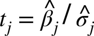
which is our estimate of ![]() divided by our estimate of its standard error, follows a Student’s t-distribution with “
divided by our estimate of its standard error, follows a Student’s t-distribution with “![]() degrees of freedom.”
degrees of freedom.”
defp_value(beta_hat_j,sigma_hat_j):
ifbeta_hat_j>0:
# if the coefficient is positive, we need to compute twice the
# probability of seeing an even *larger* value
return2*(1-normal_cdf(beta_hat_j/sigma_hat_j))
else:
# otherwise twice the probability of seeing a *smaller* value
return2*normal_cdf(beta_hat_j/sigma_hat_j)
p_value(30.63,1.174)# ~0 (constant term)
p_value(0.972,0.079)# ~0 (num_friends)
p_value(-1.868,0.131)# ~0 (work_hours)
p_value(0.911,0.990)# 0.36 (phd)
In more elaborate regression scenarios, you sometimes want to test more elaborate hypotheses about the data, such as “at least one of the ![]() is non-zero” or “
is non-zero” or “![]() equals
equals ![]() and
and ![]() equals
equals ![]() ,” which you can do with an F-test, which, alas, falls outside the scope of this book.
,” which you can do with an F-test, which, alas, falls outside the scope of this book.
# alpha is a *hyperparameter* controlling how harsh the penalty is# sometimes it's called "lambda" but that already means something in Pythondefridge_penalty(beta,alpha):
returnalpha*dot(beta[1:],beta[1:])
defsquared_error_ridge(x_i,y_i,beta,alpha):
"""estimate error plus ridge penalty on beta"""
returnerror(x_i,y_i,beta)**2+ridge_penalty(beta,alpha)
defridge_penalty_gradient(beta,alpha):
"""gradient of just the ridge penalty"""
return[0]+[2*alpha*beta_jforbeta_jinbeta[1:]]
defsquared_error_ridge_gradient(x_i,y_i,beta,alpha):
"""the gradient corresponding to the ith squared error term
including the ridge penalty"""returnvector_add(squared_error_gradient(x_i,y_i,beta),
ridge_penalty_gradient(beta,alpha))
defestimate_beta_ridge(x,y,alpha):
"""use gradient descent to fit a ridge regression
with penalty alpha"""beta_initial=[random.random()forx_iinx[0]]
returnminimize_stochastic(partial(squared_error_ridge,alpha=alpha),
partial(squared_error_ridge_gradient,
alpha=alpha),
x,y,
beta_initial,
0.001)
random.seed(0)beta_0=estimate_beta_ridge(x,daily_minutes_good,alpha=0.0)
# [30.6, 0.97, -1.87, 0.91]dot(beta_0[1:],beta_0[1:])# 5.26
multiple_r_squared(x,daily_minutes_good,beta_0)# 0.680
beta_0_01=estimate_beta_ridge(x,daily_minutes_good,alpha=0.01)
# [30.6, 0.97, -1.86, 0.89]dot(beta_0_01[1:],beta_0_01[1:])# 5.19
multiple_r_squared(x,daily_minutes_good,beta_0_01)# 0.680
beta_0_1=estimate_beta_ridge(x,daily_minutes_good,alpha=0.1)
# [30.8, 0.95, -1.84, 0.54]dot(beta_0_1[1:],beta_0_1[1:])# 4.60
multiple_r_squared(x,daily_minutes_good,beta_0_1)# 0.680
beta_1=estimate_beta_ridge(x,daily_minutes_good,alpha=1)
# [30.7, 0.90, -1.69, 0.085]dot(beta_1[1:],beta_1[1:])# 3.69
multiple_r_squared(x,daily_minutes_good,beta_1)# 0.676
beta_10=estimate_beta_ridge(x,daily_minutes_good,alpha=10)
# [28.3, 0.72, -0.91, -0.017]dot(beta_10[1:],beta_10[1:])# 1.36
multiple_r_squared(x,daily_minutes_good,beta_10)# 0.573
NOTE
deflasso_penalty(beta,alpha):
returnalpha*sum(abs(beta_i)forbeta_iinbeta[1:])
For Further Exploration
§ Regression has a rich and expansive theory behind it. This is another place where you should consider reading a textbook or at least a lot of Wikipedia articles.
§ scikit-learn has a linear_model module that provides a LinearRegression model similar to ours, as well as Ridge regression, Lasso regression, and other types of regularization too.
§ Statsmodels is another Python module that contains (among other things) linear regression models.
All materials on the site are licensed Creative Commons Attribution-Sharealike 3.0 Unported CC BY-SA 3.0 & GNU Free Documentation License (GFDL)
If you are the copyright holder of any material contained on our site and intend to remove it, please contact our site administrator for approval.
© 2016-2026 All site design rights belong to S.Y.A.