Algorithms (2014)
One. Fundamentals
1.5 Case Study: Union-Find
TO ILLUSTRATE our basic approach to developing and analyzing algorithms, we now consider a detailed example. Our purpose is to emphasize the following themes.
• Good algorithms can make the difference between being able to solve a practical problem and not being able to address it at all.
• An efficient algorithm can be as simple to code as an inefficient one.
• Understanding the performance characteristics of an implementation can be an interesting and satisfying intellectual challenge.
• The scientific method is an important tool in helping us choose among different methods for solving the same problem.
• An iterative refinement process can lead to increasingly efficient algorithms.
These themes are reinforced throughout the book. This prototypical example sets the stage for our use of the same general methodology for many other problems.
The problem that we consider is not a toy problem; it is a fundamental computational task, and the solution that we develop is of use in a variety of applications, from percolation in physical chemistry to connectivity in communications networks. We start with a simple solution, then seek to understand that solution’s performance characteristics, which help us to see how to improve the algorithm.
Dynamic connectivity
We start with the following problem specification: The input is a sequence of pairs of integers, where each integer represents an object of some type and we are to interpret the pair p q as meaning “p is connected to q.” We assume that “is connected to” is an equivalence relation, which means that it is
• Reflexive: p is connected to p.
• Symmetric: If p is connected to q, then q is connected to p.
• Transitive: If p is connected to q and q is connected to r, then p is connected to r.
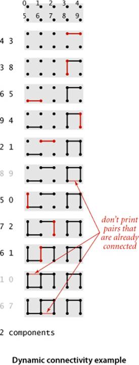
An equivalence relation partitions the objects into equivalence classes. In this case, two objects are in the same equivalence class if and only if they are connected. Our goal is to write a program to filter out extraneous pairs (pairs where both objects are in the same equivalence class) from the sequence. In other words, when the program reads a pair p q from the input, it should write the pair to the output only if the pairs it has seen to that point do not imply that p is connected to q. If the previous pairs do imply that p is connected to q, then the program should ignore the pair p q and proceed to read in the next pair. The figure on the facing page gives an example of this process. To achieve the desired goal, we need to devise a data structure that can remember sufficient information about the pairs it has seen to be able to decide whether or not a new pair of objects is connected. Informally, we refer to the task of designing such a method as the dynamic connectivity problem. This problem arises applications such as the following:
Networks
The integers might represent computers in a large network, and the pairs might represent connections in the network. Then, our program determines whether we need to establish a new direct connection for p and q to be able to communicate or whether we can use existing connections to set up a communications path. Or, the integers might represent contact sites in an electrical circuit, and the pairs might represent wires connecting the sites. Or, the integers might represent people in a social network, and the pairs might represent friendships. In such applications, we might need to process millions of objects and billions of connections.
Variable-name equivalence
In certain programming environments, it is possible to declare two variable names as being equivalent (references to the same object). After a sequence of such declarations, the system needs to be able to determine whether two given names are equivalent. This application is an early one (for the FORTRAN programming language) that motivated the development of the algorithms that we are about to consider.
Mathematical sets
On a more abstract level, you can think of the integers as belonging to mathematical sets. When we process a pair p q, we are asking whether they belong to the same set. If not, we unite p’s set and q’s set, putting them in the same set.
TO FIX IDEAS, we will use networking terminology for the rest of this section and refer to the objects as sites, the pairs as connections, and the equivalence classes as connected components, or just components for short. For simplicity, we assume that we have N sites with integer names, from 0to N-1. We do so without loss of generality because we shall be considering a host of algorithms in CHAPTER 3 that can associate arbitrary names with such integer identifiers in an efficient manner.
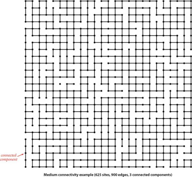
A larger example that gives some indication of the difficulty of the connectivity problem is depicted in the figure at the top of the next page. You can quickly identify the component consisting of a single site in the left middle of the diagram and the component consisting of five sites at the bottom left, but you might have difficulty verifying that all of the other sites are connected to one another. For a program, the task is even more difficult, because it has to work just with site names and connections and has no access to the geometric placement of sites in the diagram. How can we tell quickly whether or not any given two sites in such a network are connected?
The first task that we face in developing an algorithm is to specify the problem in a precise manner. The more we require of an algorithm, the more time and space we may expect it to need to finish the job. It is impossible to quantify this relationship a priori, and we often modify a problem specification on finding that it is difficult or expensive to solve or, in happy circumstances, on finding that an algorithm can provide information more useful than what was called for in the original specification. For example, our connectivity problem specification requires only that our program be able to determine whether or not any given pair p q is connected, and not that it be able to demonstrate a set of connections that connect that pair. Such a requirement makes the problem more difficult and leads us to a different family of algorithms, which we consider in SECTION 4.1.
To specify the problem, we develop an API that encapsulates the basic operations that we need: initialize, add a connection between two sites, identify the component containing a site, determine whether two sites are in the same component, and count the number of components. Thus, we articulate the following API:
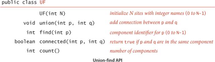
The union() operation merges two components if the two sites are in different components, the find() operation returns an integer component identifier for a given site, the connected() operation determines whether two sites are in the same component, and the count() method returns the number of components. We start with N components, and each union() that merges two different components decrements the number of components by 1.
As we shall soon see, the development of an algorithmic solution for dynamic connectivity thus reduces to the task of developing an implementation of this API. Every implementation has to
• Define a data structure to represent the known connections
• Develop efficient union(), find(), connected(), and count() implementations that are based on that data structure
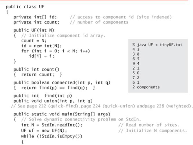
As usual, the nature of the data structure has a direct impact on the efficiency of the algorithms, so data structure and algorithm design go hand in hand. The API already specifies the convention that both sites and components will be identified by int values between 0 and N-1, so it makes sense to use a site-indexed array id[] as our basic data structure to represent the components. We always use the name of one of the sites in a component as the component identifier, so you can think of each component as being represented by one of its sites. Initially, we start with N components, each site in its own component, so we initialize id[i] to i for all i from 0 to N-1. For each site i, we keep the information needed by find() to determine the component containing i in id[i], using various algorithm-dependent strategies. All of our implementations use a one-line implementation ofconnected() that returns the boolean value find(p) == find(q).
IN SUMMARY, our starting point is ALGORITHM 1.5 on the facing page. We maintain two instance variables, the count of components and the array id[]. Implementations of find() and union() are the topic of the remainder of this section.
% more tinyUF.txt
10
4 3
3 8
6 5
9 4
2 1
8 9
5 0
7 2
6 1
1 0
6 7
% more mediumUF.txt
625
528 503
548 523
...
[900 connections]
% more largeUF.txt
1000000
786321 134521
696834 98245
...
[2000000 connections]
To test the utility of the API and to provide a basis for development, we include a client in main() that uses it to solve the dynamic connectivity problem. It reads the value of N followed by a sequence of pairs of integers (each in the range 0 to N-1), calling connected() for each pair: If the two sites in the pair are already connected, it moves on to the next pair; if they are not, it calls union() and prints the pair. Before considering implementations, we also prepare test data: the file tinyUF.txt contains the 11 connections among 10 sites used in the small example illustrated on page 217, the filemediumUF.txt contains the 900 connections among 625 sites illustrated on page 218, and the file largeUF.txt is an example with 2 million connections among 1 millions sites. Our goal is to be able to handle inputs such as largeUF.txt in a reasonable amount of time.
To analyze the algorithms, we focus on the number of times each algorithm accesses an array entry. By doing so, we are implicitly formulating the hypothesis that the running times of the algorithms on a particular machine are within a constant factor of this quantity. This hypothesis is immediate from the code, is not difficult to validate through experimentation, and provides a useful starting point for comparing algorithms, as we will see.
Union-find cost model. When studying algorithms to implement the union-find API, we count array accesses (the number of times an array entry is accessed, for read or write).
Algorithm 1.5 Union-find implementation
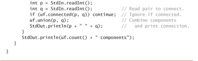
Our UF implementations are based on this code, which maintains an array of integers id[] such that the find() method returns the same integer for every site in each connected component. The union() method must maintain this invariant.
Implementations
We shall consider three different implementations, all based on using the site-indexed id[] array, to determine whether two sites are in the same connected component.
Quick-find
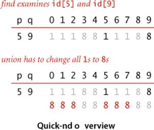
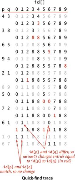
One approach is to maintain the invariant that p and q are connected if and only if id[p] is equal to id[q]. In other words, all sites in a component must have the same value in id[]. This method is called quick-find because find(p) just returns id[p], which immediately implies that connected(p, q)reduces to just the test id[p] == id[q] and returns true if and only if p and q are in the same component. To maintain the invariant for the call union(p, q), we first check whether they are already in the same component, in which case there is nothing to do. Otherwise, we are faced with the situation that all of the id[] entries corresponding to sites in the same component as p have one value and all of the id[] entries corresponding to sites in the same component as q have another value. To combine the two components into one, we have to make all of the id[] entries corresponding to both sets of sites the same value, as shown in the example at right. To do so, we go through the array, changing all the entries with values equal to id[p] to the value id[q]. We could have decided to change all the entries equal to id[q] to the value id[p]—the choice between these two alternatives is arbitrary. The code for find() and union() based on these descriptions, given at left, is straightforward. A full trace for our development client with our sample test data tinyUF.txt is shown on the next page.
Quick-find
public int find(int p)
{ return id[p]; }
public void union(int p, int q)
{ // Put p and q into the same component.
int pID = find(p);
int qID = find(q);
// Nothing to do if p and q are already
in the same component.
if (pID == qID) return;
Change values from id[p] to id[q].
for (int i = 0; i < id.length; i++)
if (id[i] == pID) id[i] = qID;
count--;
}
Quick-find analysis.
The find() operation is certainly quick, as it only accesses the id[] array once in order to complete the operation. But quick-find is typically not useful for large problems because union() needs to scan through the whole id[] array for each input pair.
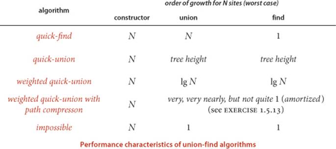
Proposition F. The quick-find algorithm uses one array access for each call to find(), two array accesses for each call to connected(), and between N + 3 and 2N + 1 array accesses for each call to union() that combines two components.
Proof: Immediate from the code. Each call to connected() tests two entries in the id[] array, one for each of the two calls to find(). Each call to union() that combines two components does so by making two calls to find(), testing each of the N entries in the id[] array, and changing between 1 and N−1 of them.
In particular, suppose that we use quick-find for the dynamic connectivity problem and wind up with a single component. This requires at least N−1 calls to union(), and, consequently, at least (N+3)(N−1) ~ N2 array accesses—we are led immediately to the hypothesis that dynamic connectivity with quick-find can be a quadratic-time process. This analysis generalizes to say that quick-find is quadratic for typical applications where we end up with a small number of components. You can easily validate this hypothesis on your computer with a doubling test (see EXERCISE 1.5.23 for an instructive example). Modern computers can execute hundreds of millions or billions of instructions per second, so this cost is not noticeable if N is small, but we also might find ourselves with millions or billions of sites and connections to process in a modern application, as represented by our test file largeUF.txt. If you are still not convinced and feel that you have a particularly fast computer, try using quick-find to determine the number of components implied by the pairs in largeUF.txt. The inescapable conclusion is that we cannot feasibly solve such a problem using the quick-find algorithm, so we seek better algorithms.
Quick-union
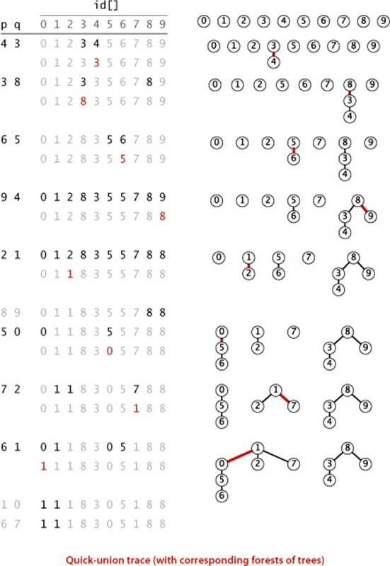
The next algorithm that we consider is a complementary method that concentrates on speeding up the union() operation. It is based on the same data structure—the site-indexed id[] array—but we interpret the values differently, to define more complicated structures. Specifically, the id[] entry for each site is the name of another site in the same component (possibly itself)—we refer to this connection as a link. To implement find(), we start at the given site, follow its link to another site, follow that site’s link to yet another site, and so forth, following links until reaching a root, a site that has a link to itself (which is guaranteed to happen, as you will see). Two sites are in the same component if and only if this process leads them to the same root. To validate this process, we need union(p, q) to maintain this invariant, which is easily arranged: we follow links to find the roots associated with p and q, then rename one of the components by linking one of these roots to the other; hence the name quick-union. Again, we have an arbitrary choice of whether to rename the component containing p or the component containing q; the implementation above renames the one containing p. The figure on the next page shows a trace of the quick-union algorithm for tinyUF.txt. This trace is best understood in terms of the graphical representation depicted at left, which we consider next.
Quick-union
public int find(int p)
{ // Find component name.
while (p != id[p]) p = id[p];
return p;
}
public void union(int p, int q)
{ // Give p and q the same root.
int i = find(p);
int j = find(q);
if (i == j) return;
id[i] = j;
count--;
}

Forest-of-trees representation
The code for quick-union is compact, but a bit opaque. Representing sites as nodes (labeled circles) and links as arrows from one node to another gives a graphical representation of the data structure that makes it relatively easy to understand the operation of the algorithm. The resulting structures are trees—in technical terms, our id[] array is a parent-link representation of a forest (set) of trees. To simplify the diagrams, we often omit both the arrowheads in the links (because they all point upwards) and the self-links in the roots of the trees. The forests corresponding to theid[] array for tinyUF.txt are shown at right. When we start at the node corresponding to any site and follow links, we eventually end up at the root of the tree containing that node. We can prove this property to be true by induction: It is true after the array is initialized to have every node link to itself, and if it is true before a given union() operation, it is certainly true afterward. Thus, the find() method on page 224 returns the name of the site at the root (so that connected() checks whether two sites are in the same tree). This representation is useful for this problem because the nodes corresponding to two sites are in the same tree if and only if the sites are in the same component. Moreover, the trees are not difficult to build: the union() implementation on page 224 combines two trees into one in a single statement, by making the root of one the parent of the other.
Quick-union analysis
The quick-union algorithm would seem to be faster than the quick-find algorithm, because it does not have to go through the entire array for each input pair; but how much faster is it? Analyzing the cost of quick-union is more difficult than it was for quick-find, because the cost is more dependent on the nature of the input. In the best case, find() just needs one array access to find the identifier associated with a site, as in quick-find; in the worst case, it needs 2N − 1 array accesses, as for 0 in the example at left (this count is conservative since compiled code will typically notdo an array access for the second reference to id[p] in the while loop). Accordingly, it is not difficult to construct a best-case input for which the running time of our dynamic connectivity client is linear; on the other hand it is also not difficult to construct a worst-case input for which the running time is quadratic (see the diagram at left and PROPOSITION G below). Fortunately, we do not need to face the problem of analyzing quick union and we will not dwell on comparative performance of quick-find and quick-union because we will next examine another variant that is far more efficient than either. For the moment, you can regard quick-union as an improvement over quick-find because it removes quick-find’s main liability (that union() always takes linear time). This difference certainly represents an improvement for typical data, but quick-union still has the liability that we cannot guarantee it to be substantially faster than quick-find in every case (for certain input data, quick-union is no faster than quick-find).
Definition. The size of a tree is its number of nodes. The depth of a node in a tree is the number of links on the path from it to the root. The height of a tree is the maximum depth among its nodes.
Proposition G. The number of array accesses used by find() in quick-union is 1 plus the twice the depth of the node corresponding to the given site. The number of array accesses used by union() and connected() is the cost of the two find() operations (plus 1 for union() if the given sites are in different trees).
Proof: Immediate from the code.
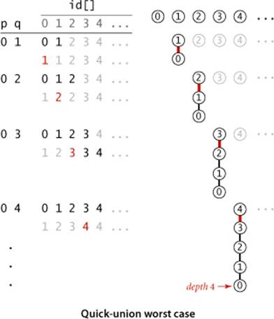
Again, suppose that we use quick-union for the dynamic connectivity problem and wind up with a single component. An immediate implication of PROPOSITION G is that the running time is quadratic, in the worst case. Suppose that the input pairs come in the order 0-1, then 0-2, then 0-3, and so forth. After N−1 such pairs, we have N sites all in the same set, and the tree that is formed by the quick-union algorithm has height N−1, with 0 linking to 1, which links to 2, which links to 3, and so forth (see the diagram on the facing page). By PROPOSITION G, the number of array accesses for the union() operation for the pair 0 i is exactly 2i + 3 (site 0 is at depth i and site i at depth 0). Thus, the total number of array accesses for the find() operations for these N pairs is (3 + 7 + 7+ . . . +2N+1) ~N2.
Weighted quick-union
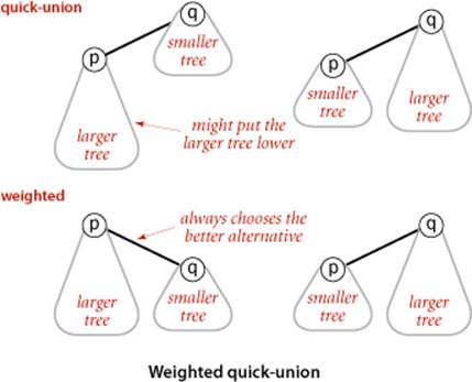
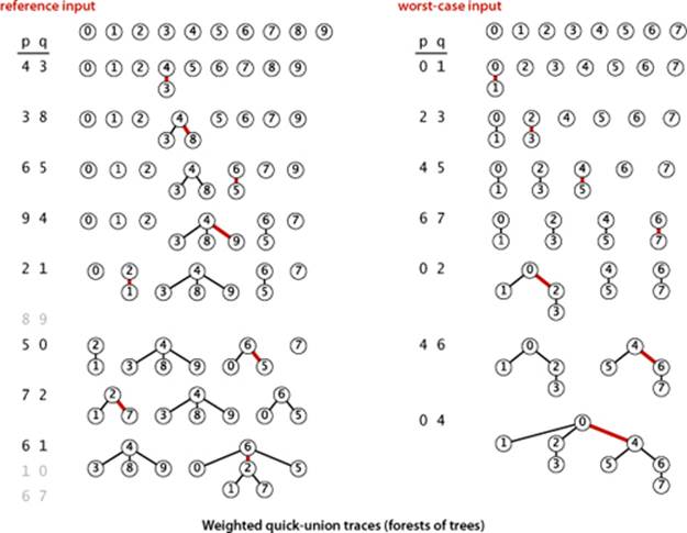
Fortunately, there is an easy modification to quick-union that allows us to guarantee that bad cases such as this one do not occur. Rather than arbitrarily connecting the second tree to the first for union(), we keep track of the size of each tree and always connect the smaller tree to the larger. This change requires slightly more code and another array to hold the node counts, as shown on page 228, but it leads to substantial improvements in efficiency. We refer to this algorithm as the weighted quick-union algorithm. The forest of trees constructed by this algorithm for tinyUF.txt is shown in the figure at left on the top of page 229. Even for this small example, the tree height is substantially smaller than the height for the unweighted version.
Weighted quick-union analysis
The figure at right on the top of page 229 illustrates the worst case for weighted quick union, when the sizes of the trees to be merged by union() are always equal (and a power of 2). These tree structures look complex, but they have the simple property that the height of a tree of 2n nodes is n. Furthermore, when we merge two trees of 2n nodes, we get a tree of 2n+1 nodes, and we increase the height of the tree to n+1. This observation generalizes to provide a proof that the weighted algorithm can guarantee logarithmic performance.
% java WeightedQuickUnionUF < mediumUF.txt
528 503
548 523
...
3 components
% java WeightedQuickUnionUF < largeUF.txt
786321 134521
696834 98245
...
6 components
Algorithm 1.5 Union-find implementation (weighted quick-union)
public class WeightedQuickUnionUF
{
private int[] id; // parent link (site indexed)
private int[] sz; // size of component for roots (site indexed)
private int count; // number of components
public WeightedQuickUnionUF(int N)
{
count = N;
id = new int[N];
for (int i = 0; i < N; i++) id[i] = i;
sz = new int[N];
for (int i = 0; i < N; i++) sz[i] = 1;
}
public int count()
{ return count; }
public boolean connected(int p, int q)
{ return find(p) == find(q); }
public int find(int p)
{ // Follow links to find a root.
while (p != id[p]) p = id[p];
return p;
}
public void union(int p, int q)
{
int i = find(p);
int j = find(q);
if (i == j) return;
// Make smaller root point to larger one.
if (sz[i] < sz[j]) { id[i] = j; sz[j] += sz[i]; }
else { id[j] = i; sz[i] += sz[j]; }
count--;
}
}
This code is best understood in terms of the forest-of-trees representation described in the text. We add a site-indexed array sz[] as an instance variable so that union() can link the root of the smaller tree to the root of the larger tree. This addition makes it feasible to address large problems.
Proposition H. The depth of any node in a forest built by weighted quick-union for N sites is at most lg N.
Proof: We prove a stronger fact by (strong) induction: The height of every tree of size k in the forest is at most lg k. The base case follows from the fact that the tree height is 0 when k is 1. By the inductive hypothesis, assume that the tree height of a tree of size i is at most lg i for all i < k. When we combine a tree of size i with a tree of size j with i ≤ j and i+j = k, we increase the depth of each node in the smaller set by 1, but they are now in a tree of size i+j = k, so the property is preserved because 1+lg i = lg(i+i) ≤ lg(i+j) = lg k.
Corollary. For weighted quick-union with N sites, the worst-case order of growth of the cost of find(), connected(), and union() is log N.
Proof. Each operation does at most a constant number of array accesses for each node on the path from a node to a root in the forest.
For dynamic connectivity, the practical implication of PROPOSITION H and its corollary is that weighted quick-union is the only one of the three algorithms that can feasibly be used for huge practical problems. The weighted quick-union algorithm uses at most c M lg N array accesses to processM connections among N sites for a small constant c. This result is in stark contrast to our finding that quick-find always (and quick-union sometimes) uses at least MN array accesses. Thus, with weighted quick-union, we can guarantee that we can solve huge practical dynamic connectivity problems in a reasonable amount of time. For the price of a few extra lines of code, we get a program that can be millions of times faster than the simpler algorithms for the huge dynamic connectivity problems that we might encounter in practical applications.
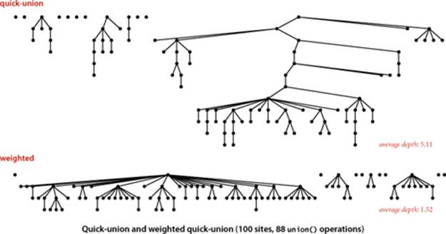
A 100-site example is shown on the top of this page. It is evident from this diagram that relatively few nodes fall far from the root with weighted quick-union. Indeed it is frequently the case that a 1-node tree is merged with a larger tree, which puts the node just one link from the root. Empirical studies on huge problems tell us that weighted quick-union typically solves practical problems in constant time per operation. We could hardly expect to find a more efficient algorithm.
Optimal algorithms
Can we find an algorithm that has guaranteed constant-time-per-operation performance? This question is an extremely difficult one that plagued researchers for many years. In pursuit of an answer, a number of variations of quick-union and weighted quick-union have been studied. For example, the following method, known as path compression, is easy to implement. Ideally, we would like every node to link directly to the root of its tree, but we do not want to pay the price of changing a large number of links, as we did in the quick-find algorithm. We can approach the ideal simply by making all the nodes that we do examine directly link to the root. This step seems drastic at first blush, but it is easy to implement, and there is nothing sacrosanct about the structure of these trees: if we can modify them to make the algorithm more efficient, we should do so. To implement path compression, we just add another loop to find() that sets the id[] entry corresponding to each node encountered along the way to link directly to the root. The net result is to flatten the trees almost completely, approximating the ideal achieved by the quick-find algorithm. The method is simple and effective, but you are not likely to be able to discern any improvement over weighted quick-union in a practical situation (see EXERCISE 1.5.24). Theoretical results about the situation are extremely complicated and quite remarkable. Weighted quick union with path compression is optimal but not quite constant-time per operation. That is, not only is weighted quick-union with path compression not constant-time per operation in the worst case (amortized), but also there exists no algorithm that can guarantee to perform each union-find operation in amortized constant time (under the very general “cell probe” model of computation). Weighted quick-union with path compression is very close to the best that we can do for this problem.
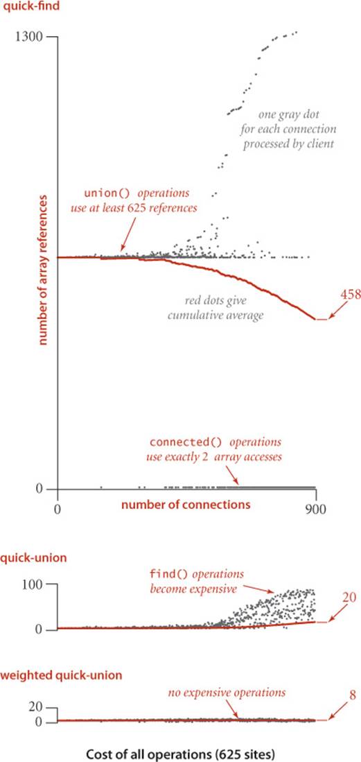
Amortized cost plots
As with any data type implementation, it is worthwhile to run experiments to test the validity of our performance hypotheses for typical clients, as discussion in SECTION 1.4. The figure at left shows details of the performance of the algorithms for our dynamic connectivity development client when solving our 625-site connectivity example (mediumUF.txt). Such diagrams are easy to produce (see EXERCISE 1.5.16): For the ith connection processed, we maintain a variable cost that counts the number of array accesses (to id[] or sz[]) and a variable total that is the sum of the total number of array accesses so far. Then we plot a gray dot at (i, cost) and a red dot at (i, total/i). The red dots are the average cost per operation, or amortized cost. These plots provide good insights into algorithm behavior. For quick-find, every union() operation uses at least 625 accesses (plus 1 for each component merged, up to another 625) and every connected() operation uses 2 accesses. Initially, most of the connections lead to a call on union(), so the cumulative average hovers around 625; later, most connections are calls to connected() that cause the call to union() to be skipped, so the cumulative average decreases, but still remains relatively high. (Inputs that lead to a large number of connected() calls that cause union() to be skipped will exhibit significantly better performance—see EXERCISE 1.5.23 for an example). For quick-union, all operations initially require only a few array accesses; eventually, the height of the trees becomes a significant factor and the amortized cost grows noticably. For weighted quick-union, the tree height stays small, none of the operations are expensive, and the amortized cost is low. These experiments validate our conclusion that weighted quick-union is certainly worth implementing and that there is not much further room for improvement for practical problems.
Perspective
Each of the UF implementations that we considered is an improvement over the previous in some intuitive sense, but the process is artificially smooth because we have the benefit of hindsight in looking over the development of the algorithms as they were studied by researchers over the years. The implementations are simple and the problem is well specified, so we can evaluate the various algorithms directly by running empirical studies. Furthermore, we can use these studies to validate mathematical results that quantify the performance of these algorithms. When possible, we follow the same basic steps for fundamental problems throughout the book that we have taken for union–find algorithms in this section, some of which are highlighted in this list:
• Decide on a complete and specific problem statement, including identifying fundamental abstract operations that are intrinsic to the problem and an API.
• Carefully develop a succinct implementation for a straightforward algorithm, using a well-thought-out development client and realistic input data.
• Know when an implementation could not possibly be used to solve problems on the scale contemplated and must be improved or abandoned.
• Develop improved implementations through a process of stepwise refinement, validating the efficacy of ideas for improvement through empirical analysis, mathematical analysis, or both.
• Find high-level abstract representations of data structures or algorithms in operation that enable effective high-level design of improved versions.
• Strive for worst-case performance guarantees when possible, but accept good performance on typical data when available.
• Know when to leave further improvements for detailed in-depth study to skilled researchers and move on to the next problem.
The potential for spectacular performance improvements for practical problems such as those that we saw for union–find makes algorithm design a compelling field of study. What other design activities hold the potential to reap savings factors of millions or billions, or more?
Developing an efficient algorithm is an intellectually satisfying activity that can have direct practical payoff. As the dynamic connectivity problem indicates, a simply stated problem can lead us to study numerous algorithms that are not only both useful and interesting, but also intricate and challenging to understand. We shall encounter many ingenious algorithms that have been developed over the years for a host of practical problems. As the scope of applicability of computational solutions to scientific and commercial problems widens, so also grows the importance of being able to use efficient algorithms to solve known problems and of being able to develop efficient solutions to new problems.
Q&A
Q. I’d like to add a delete() method to the API that allows clients to delete connections. Any advice on how to proceed?
A. No one has devised an algorithm as simple and efficient as the ones in this section that can handle deletions. This theme recurs throughout this book. Several of the data structures that we consider have the property that deleting something is much more difficult than adding something.
Q. What is the cell-probe model?
A. A model of computation where we only count accesses to a random-access memory large enough to hold the input and consider all other operations to be free.
Exercises
1.5.1 Show the contents of the id[] array and the number of times the array is accessed for each input pair when you use quick-find for the sequence 9-0 3-4 5-8 7-2 2-1 5-7 0-3 4-2.
1.5.2 Do EXERCISE 1.5.1, but use quick-union (page 224). In addition, draw the forest of trees represented by the id[] array after each input pair is processed.
1.5.3 Do EXERCISE 1.5.1, but use weighted quick-union (page 228).
1.5.4 Show the contents of the sz[] and id[] arrays and the number of array accesses for each input pair corresponding to the weighted quick-union examples in the text (both the reference input and the worst-case input).
1.5.5 Estimate the minimum amount of time (in days) that would be required for quick-find to solve a dynamic connectivity problem with 109 sites and 106 input pairs, on a computer capable of executing 109 instructions per second. Assume that each iteration of the inner for loop requires 10 machine instructions.
1.5.6 Repeat EXERCISE 1.5.5 for weighted quick-union.
1.5.7 Develop classes QuickUnionUF and QuickFindUF that implement quick-union and quick-find, respectively.
1.5.8 Give a counterexample that shows why this intuitive implementation of union() for quick-find is not correct:
public void union(int p, int q)
{
if (connected(p, q)) return;
// Rename p's component to q's name.
for (int i = 0; i < id.length; i++)
if (id[i] == id[p]) id[i] = id[q];
count--;
}
1.5.9 Draw the tree corresponding to the id[] array depicted at right. Can this be the result of running weighted quick-union? Explain why this is impossible or give a sequence of operations that results in this array.
![]()
1.5.10 In the weighted quick-union algorithm, suppose that we set id[find(p)] to q instead of to id[find(q)]. Would the resulting algorithm be correct?
Answer: Yes, but it would increase the tree height, so the performance guarantee would be invalid.
1.5.11 Implement weighted quick-find, where you always change the id[] entries of the smaller component to the identifier of the larger component. How does this change affect performance?
Creative Problems
1.5.12 Quick-union with path compression. Modify quick-union (page 224) to include path compression, by adding a loop to find() that links every site on the path from p to the root. Give a sequence of input pairs that causes this method to produce a path of length 4. Note : The amortized cost per operation for this algorithm is known to be logarithmic.
1.5.13 Weighted quick-union with path compression. Modify weighted quick-union (ALGORITHM 1.5) to implement path compression, as described in EXERCISE 1.5.12. Give a sequence of input pairs that causes this method to produce a tree of height 4. Note: The amortized cost per operation for this algorithm is known to be bounded by a function known as the inverse Ackermann function and is less than 5 for any conceivable practical value of N.
1.5.14 Weighted quick-union by height. Develop a UF implementation that uses the same basic strategy as weighted quick-union but keeps track of tree height and always links the shorter tree to the taller one. Prove a logarithmic upper bound on the height of the trees for N sites with your algorithm.
1.5.15 Binomial trees. Show that the number of nodes at each level in the worst-case trees for weighted quick-union are binomial coefficients. Compute the average depth of a node in a worst-case tree with N = 2n nodes.
1.5.16 Amortized costs plots. Instrument your implementations from EXERCISE 1.5.7 to make amortized costs plots like those in the text.
1.5.17 Random connections. Develop a UF client ErdosRenyi that takes an integer value N from the command line, generates random pairs of integers between 0 and N-1, calling connected() to determine if they are connected and then union() if not (as in our development client), looping until all sites are connected, and printing the number of connections generated. Package your program as a static method count() that takes N as argument and returns the number of connections and a main() that takes N from the command line, calls count(), and prints the returned value.
1.5.18 Random grid generator. Write a program RandomGrid that takes an int value N from the command line, generates all the connections in an N-by-N grid, puts them in random order, randomly orients them (so that p q and q p are equally likely to occur), and prints the result to standard output. To randomly order the connections, use a RandomBag (see EXERCISE 1.3.34 on page 167). To encapsulate p and q in a single object, use the Connection nested class shown below. Package your program as two static methods: generate(), which takes N as argument and returns an array of connections, andmain(), which takes N from the command line, calls generate(), and iterates through the returned array to print the connections.
1.5.19 Animation. Write a RandomGrid client (see EXERCISE 1.5.18) that uses UnionFind as in our development client to check connectivity and uses StdDraw to draw the connections as they are processed.
1.5.20 Dynamic growth. Using linked lists or a resizing array, develop a weighted quick-union implementation that removes the restriction on needing the number of objects ahead of time. Add a method newSite() to the API, which returns an int identifier.
Record to encapsulate connections
private class Connection
{
int p;
int q;
public Connection(int p, int q)
{ this.p = p; this.q = q; }
}
Experiments
1.5.21 Erdös-Renyi model. Use your client from EXERCISE 1.5.17 to test the hypothesis that the number of pairs generated to get one component is ~ ½N ln N.
1.5.22 Doubling test for Erdös-Renyi model. Develop a performance-testing client that takes an int value T from the command line and performs T trials of the following experiment: Use your client from EXERCISE 1.5.17 to generate random connections, using UnionFind to determine connectivity as in our development client, looping until all sites are connected. For each N, print the value of N, the average number of connections processed, and the ratio of the running time to the previous. Use your program to validate the hypotheses in the text that the running times for quick-find and quick-union are quadratic and weighted quick-union is near-linear.
1.5.23 Compare quick-find with quick-union for Erdös-Renyi model. Develop a performance-testing client that takes an int value T from the command line and performs T trials of the following experiment: Use your client from EXERCISE 1.5.17 to generate random connections. Save the connections, so that you can use both quick-union and quick-find to determine connectivity as in our development client, looping until all sites are connected. For each N, print the value of N and the ratio of the two running times.
1.5.24 Fast algorithms for Erdös-Renyi model. Add weighted quick-union and weighted quick-union with path compression to your tests from EXERCISE 1.5.23. Can you discern a difference between these two algorithms?
1.5.25 Doubling test for random grids. Develop a performance-testing client that takes an int value T from the command line and performs T trials of the following experiement: Use your client from EXERCISE 1.5.18 to generate the connections in an N-by-N square grid, randomly oriented and in random order, then use UnionFind to determine connectivity as in our development client, looping until all sites are connected. For each N, print the value of N, the average number of connections processed, and the ratio of the running time to the previous. Use your program to validate the hypotheses in the text that the running times for quick-find and quick-union are quadratic and weighted quick-union is near-linear. Note: As N doubles, the number of sites in the grid increases by a factor of 4, so expect a doubling factor of 16 for quadratic and 4 for linear.
1.5.26 Amortized plot for Erdös-Renyi. Develop a client that takes an int value N from the command line and does an amortized plot of the cost of all operations in the style of the plots in the text for the process of generating random pairs of integers between 0 and N-1, calling connected() to determine if they are connected and then union() if not (as in our development client), looping until all sites are connected.
All materials on the site are licensed Creative Commons Attribution-Sharealike 3.0 Unported CC BY-SA 3.0 & GNU Free Documentation License (GFDL)
If you are the copyright holder of any material contained on our site and intend to remove it, please contact our site administrator for approval.
© 2016-2026 All site design rights belong to S.Y.A.