Algorithms (2014)
Two. Sorting
2.1 Elementary Sorts 244
2.2 Mergesort 270
2.3 Quicksort 288
2.4 Priority Queues 308
2.5 Applications 336
Sorting is the process of rearranging a sequence of objects so as to put them in some logical order. For example, your credit card bill presents transactions in order by date—they were likely put into that order by a sorting algorithm. In the early days of computing, the common wisdom was that up to 30 percent of all computing cycles was spent sorting. If that fraction is lower today, one likely reason is that sorting algorithms are relatively efficient, not that sorting has diminished in relative importance. Indeed, the ubiquity of computer usage has put us awash in data, and the first step to organizing data is often to sort it. All computer systems have implementations of sorting algorithms, for use by the system and by users.
There are three practical reasons for you to study sorting algorithms, even though you might just use a system sort:
• Analyzing sorting algorithms is a thorough introduction to the approach that we use to compare algorithm performance throughout the book.
• Similar techniques are effective in addressing other problems.
• We often use sorting algorithms as a starting point to solve other problems.
More important than these practical reasons is that the algorithms are elegant, classic, and effective.
Sorting plays a major role in commercial data processing and in modern scientific computing. Applications abound in transaction processing, combinatorial optimization, astrophysics, molecular dynamics, linguistics, genomics, weather prediction, and many other fields. Indeed, a sorting algorithm (quicksort, in SECTION 2.3) was named as one of the top ten algorithms for science and engineering of the 20th century.
In this chapter, we consider several classical sorting methods and an efficient implementation of a fundamental data type known as the priority queue. We discuss the theoretical basis for comparing sorting algorithms and conclude the chapter with a survey of applications of sorting and priority queues.
2.1 Elementary Sorts
FOR OUR FIRST EXCURSION into the area of sorting algorithms, we shall study two elementary sorting methods and a variation of one of them. Among the reasons for studying these relatively simple algorithms in detail are the following: First, they provide context in which we can learn terminology and basic mechanisms. Second, these simple algorithms are more effective in some applications than the sophisticated algorithms that we shall discuss later. Third, they are useful in improving the efficiency of more sophisticated algorithms, as we will see.
Rules of the game
Our primary concern is algorithms for rearranging arrays of items where each item contains a key. The objective of the sorting algorithm is to rearrange the items such that their keys are ordered according to some well-defined ordering rule (usually numerical or alphabetical order). We want to rearrange the array so that each entry’s key is no smaller than the key in each entry with a lower index and no larger than the key in each entry with a larger index. Specific characteristics of the keys and the items can vary widely across applications. In Java, items are just objects, and the abstract notion of a key is captured in a built-in mechanism—the Comparable interface—that is described on page 247.
The class Example on the facing page illustrates the conventions that we shall use: we put our sort code in a sort() method within a single class along with private helper functions less() and exch() (and perhaps some others) and a sample client main(). Example also illustrates code that might be useful for initial debugging: its test client main() sorts strings from standard input using the private method show() to print the contents of the array. Later in this chapter, we will examine various test clients for comparing algorithms and for studying their performance. To differentiate sorting methods, we give our various sort classes different names. Clients can call different implementations by name: Insertion.sort(), Merge.sort(), Quick.sort(), and so forth.
With but a few exceptions, our sort code refers to the data only through two operations: the method less() that compares items and the method exch() that exchanges them. The exch() method is easy to implement, and the Comparable interface makes it easy to implement less(). Restricting data access to these two operations makes our code readable and portable, and makes it easier for us certify that algorithms are correct, to study performance and to compare algorithms. Before proceeding to consider sort implementations, we discuss a number of important issues that need to be carefully considered for every sort.
Template for sort classes
public class Example
{
public static void sort(Comparable[] a)
{ /* See Algorithms 2.1, 2.2, 2.3, 2.4, 2.5, or 2.7. */ }
private static boolean less(Comparable v, Comparable w)
{ return v.compareTo(w) < 0; }
private static void exch(Comparable[] a, int i, int j)
{ Comparable t = a[i]; a[i] = a[j]; a[j] = t; }
private static void show(Comparable[] a)
{ // Print the array, on a single line.
for (int i = 0; i < a.length; i++)
StdOut.print(a[i] + " ");
StdOut.println();
}
public static boolean isSorted(Comparable[] a)
{ // Test whether the array entries are in order.
for (int i = 1; i < a.length; i++)
if (less(a[i], a[i-1])) return false;
return true;
}
public static void main(String[] args)
{ // Read strings from standard input, sort them, and print.
String[] a = In.readStrings();
sort(a);
assert isSorted(a);
show(a);
}
}
% more tiny.txt
S O R T E X A M P L E
% java Example < tiny.txt
A E E L M O P R S T X
% more words3.txt
bed bug dad yes zoo ... all bad yet
% java Example < words3.txt
all bad bed bug dad ... yes yet zoo
This class illustrates our conventions for implementing array sorts. For each sorting algorithm that we consider, we present a sort() method for a class like this with Example changed to a name that corresponds to the algorithm. The test client sorts strings taken from standard input, but, with this code, our sort methods are effective for any type of data that implements Comparable.
Certification
Does the sort implementation always put the array in order, no matter what the initial order? As a conservative practice, we include the statement assert isSorted(a); in our test client to certify that array entries are in order after the sort. It is reasonable to include this statement in every sort implementation, even though we normally test our code and develop mathematical arguments that our algorithms are correct. Note that this test is sufficient only if we use exch() exclusively to change array entries. When we use code that stores values into the array directly, we do not have full assurance (for example, code that destroys the original input array by setting all values to be the same would pass this test).
Running time
We also test algorithm performance. We start by proving facts about the number of basic operations (compares and exchanges, or perhaps the number of times the array is accessed, for read or write) that the various sorting algorithms perform for various natural input models. Then we use these facts to develop hypotheses about the comparative performance of the algorithms and present tools that you can use to experimentally check the validity of such hypotheses. We use a consistent coding style to facilitate the development of valid hypotheses about performance that will hold true for typical implementations.
Searching cost model. When studying sorting algorithms, we count compares and exchanges. For algorithms that do not use exchanges, we count array accesses.
Extra memory
The amount of extra memory used by a sorting algorithm is often as important a factor as running time. The sorting algorithms divide into two basic types: those that sort in place and use no extra memory except perhaps for a small function-call stack or a constant number of instance variables, and those that need enough extra memory to hold another copy of the array to be sorted.
Types of data
Our sort code is effective for any item type that implements the Comparable interface. Adhering to Java’s convention in this way is convenient because many of the types of data that you might want to sort implement Comparable. For example, Java’s numeric wrapper types such as Integer and Doubleimplement Comparable, as do String and various advanced types such as File or URL. Thus, you can just call one of our sort methods with an array of any of these types as argument. For example, the code at right uses quicksort (see SECTION 2.3) to sort N random Double values. When we create types of our own, we can enable client code to sort that type of data by implementing the Comparable interface. To do so, we just need to implement a compareTo() method that defines an ordering on objects of that type known as the natural order for that type, as shown here for our Date data type (see page91). Java’s convention is that the call v.compareTo(w) returns an integer that is negative, zero, or positive (usually -1, 0, or +1) when v < w, v = w, or v > w, respectively. For economy, we use standard notation like v>w as shorthand for code like v.compareTo(w)>0 for the remainder of this paragraph. By convention, v.compareTo(w) throws an exception if v and w are incompatible types or either is null. Furthermore, compareTo() must implement a total order: it must be
• Reflexive (for all v, v = v)
• Antisymmetric (for all v and w, if v < w then w > v and if v = w then w = v)
• Transitive (for all v, w, and x, if v <= w and w <= x then v <=x)
Sorting an array of random values
Double a[] = new Double[N];
for (int i = 0; i < N; i++)
a[i] = StdRandom.uniform();
Quick.sort(a);
Defining a comparable type
public class Date implements Comparable<Date>
{
private final int day;
private final int month;
private final int year;
public Date(int d, int m, int y)
{ day = d; month = m; year = y; }
public int day() { return day; }
public int month() { return month; }
public int year() { return year; }
public int compareTo(Date that)
{
if (this.year > that.year ) return +1;
if (this.year < that.year ) return -1;
if (this.month > that.month) return +1;
if (this.month < that.month) return -1;
if (this.day > that.day ) return +1;
if (this.day < that.day ) return -1;
return 0;
}
public String toString()
{ return month + "/" + day + "/" + year; }
}
These rules are intuitive and standard in mathematics—you will have little difficulty adhering to them. In short, compareTo() implements our key abstraction—it defines the ordering of the items (objects) to be sorted, which can be any type of data that implements Comparable. Note that compareTo()need not use all of the instance variables. Indeed, the key might be a small part of each item.
FOR THE REMAINDER OF THIS CHAPTER, we shall address numerous algorithms for sorting arrays of objects having a natural order. To compare and contrast the algorithms, we shall examine a number of their properties, including the number of compares and exchanges that they use for various types of inputs and the amount of extra memory that they use. These properties lead to the development of hypotheses about performance properties, many of which have been validated on countless computers over the past several decades. Specific implementations always need to be checked, so we also consider tools for doing so. After considering the classic selection sort, insertion sort, shellsort, mergesort, quicksort, and heapsort algorithms, we will consider practical issues and applications, in SECTION 2.5.
Selection sort
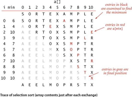
One of the simplest sorting algorithms works as follows: First, find the smallest item in the array and exchange it with the first entry (itself if the first entry is already the smallest). Then, find the next smallest item and exchange it with the second entry. Continue in this way until the entire array is sorted. This method is called selection sort because it works by repeatedly selecting the smallest remaining item.
As you can see from the implementation in ALGORITHM 2.1, the inner loop of selection sort is just a compare to test a current item against the smallest item found so far (plus the code necessary to increment the current index and to check that it does not exceed the array bounds); it could hardly be simpler. The work of moving the items around falls outside the inner loop: each exchange puts an item into its final position, so the number of exchanges is N. Thus, the running time is dominated by the number of compares.
Proposition A. Selection sort uses ~N2/2 compares and N exchanges to sort an array of length N.
Proof: You can prove this fact by examining the trace, which is an N-by-N table in which unshaded letters correspond to compares. About one-half of the entries in the table are unshaded—those on and above the diagonal. The entries on the diagonal each correspond to an exchange. More precisely, examination of the code reveals that, for each i from 0 to N − 1, there is one exchange and N− 1 − i compares, so the totals are N exchanges and (N − 1) + (N − 2) + . . . + 2 + 1+ 0 = N(N − 1)/2 ~ N2/2 compares.
IN SUMMARY, selection sort is a simple sorting method that is easy to understand and to implement and is characterized by the following two signature properties:
Running time is insensitive to input
The process of finding the smallest item on one pass through the array does not give much information about where the smallest item might be on the next pass. This property can be disadvantageous in some situations. For example, the person using the sort client might be surprised to realize that it takes about as long to run selection sort for an array that is already in order or for an array with all keys equal as it does for a randomly-ordered array! As we shall see, other algorithms are better able to take advantage of initial order in the input.
Data movement is minimal
Each of the N exchanges changes the value of two array entries, so selection sort uses N exchanges—the number of exchanges is a linear function of the array size. None of the other sorting algorithms that we consider have this property (most involve linearithmic or quadratic growth).
Algorithm 2.1 Selection sort
public class Selection
{
public static void sort(Comparable[] a)
{ // Sort a[] into increasing order.
int N = a.length; // array length
for (int i = 0; i < N; i++)
{ // Exchange a[i] with smallest entry in a[i+1...N).
int min = i; // index of a minimal entry.
for (int j = i+1; j < N; j++)
if (less(a[j], a[min])) min = j;
exch(a, i, min);
}
}
// See page 245 for less(), exch(), isSorted(), and main().
}
For each i, this implementation puts the ith smallest item in a[i]. The entries to the left of position i are the i smallest items in the array and are not examined again.
Insertion sort
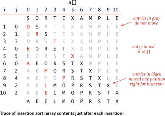
The algorithm that people often use to sort bridge hands is to consider the cards one at a time, inserting each into its proper place among those already considered (keeping them sorted). In a computer implementation, we need to make space to insert the current item by moving larger items one position to the right, before inserting the current item into the vacated position. ALGORITHM 2.2 is an implementation of this method, which is called insertion sort.
As in selection sort, the items to the left of the current index are in sorted order during the sort, but they are not in their final position, as they may have to be moved to make room for smaller items encountered later. The array is, however, fully sorted when the index reaches the right end.
Unlike that of selection sort, the running time of insertion sort depends on the initial order of the items in the input. For example, if the array is large and its entries are already in order (or nearly in order), then insertion sort is much, much faster than if the entries are randomly ordered or in reverse order.
Proposition B. Insertion sort uses ~N2/4 compares and ~N2/4 exchanges to sort a randomly ordered array of length N with distinct keys, on the average. The worst case is ~N2/2 compares and ~N2/2 exchanges and the best case is N − 1 compares and 0 exchanges.
Proof: Just as for PROPOSITION A, the number of compares and exchanges is easy to visualize in the N-by-N diagram that we use to illustrate the sort. We count entries below the diagonal—all of them, in the worst case, and none of them, in the best case. For randomly ordered arrays, we expect each item to go about halfway back, on the average, so we count one-half of the entries below the diagonal.
The number of compares is the number of exchanges plus an additional term equal to N minus the number of times the item inserted is the smallest so far. In the worst case (array in reverse order), this term is negligible in relation to the total; in the best case (array in order) it is equal to N − 1.
Insertion sort works well for certain types of nonrandom arrays that often arise in practice, even if they are huge. For example, as just mentioned, consider what happens when you use insertion sort on an array that is already sorted. Each item is immediately determined to be in its proper place in the array, and the total running time is linear. (The running time of selection sort is quadratic for such an array.) The same is true for arrays whose keys are all equal (hence the condition in PROPOSITION B that the keys must be distinct).
Algorithm 2.2 Insertion sort
public class Insertion
{
public static void sort(Comparable[] a)
{ // Sort a[] into increasing order.
int N = a.length;
for (int i = 1; i < N; i++)
{ // Insert a[i] among a[i-1], a[i-2], a[i-3]....
for (int j = i; j > 0 && less(a[j], a[j-1]); j--)
exch(a, j, j-1);
}
}
// See page 245 for less(), exch(), isSorted(), and main().
}
For each i from 1 to N-1, exchange a[i] with the entries that are larger in a[0] through a[i-1]. As the index i travels from left to right, the entries to its left are in sorted order in the array, so the array is fully sorted when i reaches the right end.
More generally, we consider the concept of a partially sorted array, as follows: An inversion is a pair of entries that are out of order in the array. For instance, E X A M P L E has 11 inversions: E-A, X-A, X-M, X-P, X-L, X-E, M-L, M-E, P-L, P-E, and L-E. If the number of inversions in an array is less than a constant multiple of the array size, we say that the array is partially sorted. Typical examples of partially sorted arrays are the following:
• An array where each entry is not far from its final position
• A small array appended to a large sorted array
• An array with only a few entries that are not in place
Insertion sort is an efficient method for such arrays; selection sort is not. Indeed, when the number of inversions is low, insertion sort is likely to be faster than any sorting method that we consider in this chapter.
Proposition C. The number of exchanges used by insertion sort is equal to the number of inversions in the array, and the number of compares is at least equal to the number of inversions and at most equal to the number of inversions plus the array size minus 1.
Proof: Every exchange involves two inverted adjacent entries and thus reduces the number of inversions by one, and the array is sorted when the number of inversions reaches zero. Every exchange corresponds to a compare, and an additional compare might happen for each value of i from 1 to N-1 (when a[i] does not reach the left end of the array).
It is not difficult to speed up insertion sort substantially, by shortening its inner loop to move the larger entries to the right one position rather than doing full exchanges (thus cutting the number of array accesses in half). We leave this improvement for an exercise (see EXERCISE 2.1.25).
IN SUMMARY, insertion sort is an excellent method for partially sorted arrays and is also a fine method for tiny arrays. These facts are important not just because such arrays frequently arise in practice, but also because both types of arrays arise in intermediate stages of advanced sorting algorithms, so we will be considering insertion sort again in relation to such algorithms.
Visualizing sorting algorithms
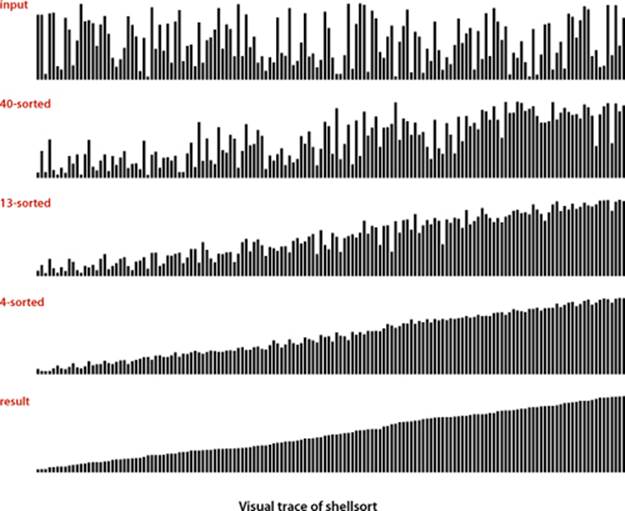
Throughout this chapter, we will be using a simple visual representation to help describe the properties of sorting algorithms. Rather than tracing the progress of a sort with key values such as letters, numbers, or words, we use vertical bars, to be sorted by their heights. The advantage of such a representation is that it can give insights into the behavior of a sorting method.
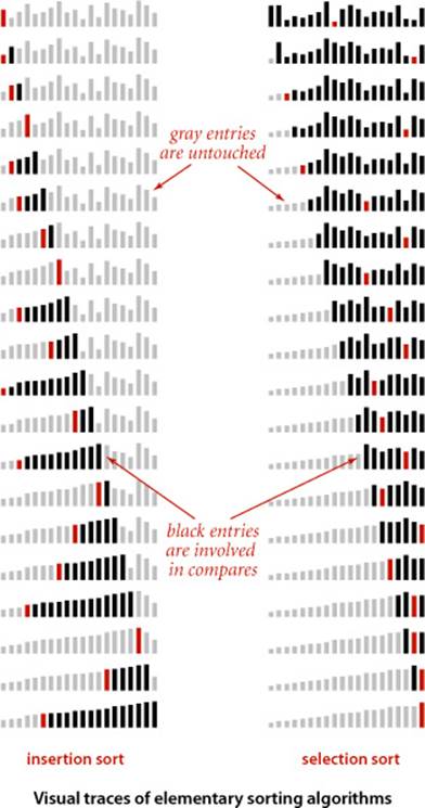
For example, you can see at a glance on the visual traces at right that insertion sort does not touch entries to the right of the scan pointer and selection sort does not touch entries to the left of the scan pointer. Moreover, it is clear from the visual traces that, since insertion sort also does not touch entries smaller than the inserted item, it uses about half the number of compares as selection sort, on the average.
With our StdDraw library, developing a visual trace is not much more difficult than doing a standard trace. We sort Double values, instrument the algorithm to call show() as appropriate (just as we do for a standard trace), and develop a version of show() that uses StdDraw to draw the bars instead of printing the results. The most complicated task is setting the scale for the y-axis so that the lines of the trace appear in the expected order. You are encouraged to work EXERCISE 2.1.18 in order to gain a better appreciation of the value of visual traces and the ease of creating them.
An even simpler task is to animate the trace so that you can see the array dynamically evolve to the sorted result. Developing an animated trace involves essentially the same process described in the previous paragraph, but without having to worry about the y-axis (just clear the window and redraw the bars each time). Though we cannot make the case on the printed page, such animated representations are also effective in gaining insight into how an algorithm works. You are also encouraged to work EXERCISE 2.1.17 to see for yourself.
Comparing two sorting algorithms
Now that we have two implementations, we are naturally interested in knowing which one is faster: selection sort (ALGORITHM 2.1) or insertion sort (ALGORITHM 2.2). Questions like this arise again and again and again in the study of algorithms and are a major focus throughout this book. We have discussed some fundamental ideas in CHAPTER 1, but we use this first case in point to illustrate our basic approach to answering such questions. Generally, following the approach introduced in SECTION 1.4, we compare algorithms by
• Implementing and debugging them
• Analyzing their basic properties
• Formulating a hypothesis about comparative performance
• Running experiments to validate the hypothesis
These steps are nothing more than the time-honored scientific method, applied to the study of algorithms.
In the present context, ALGORITHM 2.1 and ALGORITHM 2.2 are evidence of the first step; PROPOSITIONS A, B, and C constitute the second step; PROPERTY D on page 255 constitutes the third step; and the class SortCompare on page 256 enables the fourth step. These activities are all interrelated.
Our brief descriptions mask a substantial amount of effort that is required to properly implement, analyze, and test algorithms. Every programmer knows that such code is the product of a long round of debugging and refinement, every mathematician knows that proper analysis can be very difficult, and every scientist knows that formulating hypotheses and designing and executing experiments to validate them require great care. Full development of such results is reserved for experts studying our most important algorithms, but every programmer using an algorithm should be aware of the scientific context underlying its performance properties.
Having developed implementations, our next choice is to settle on an appropriate model for the input. For sorting, a natural model, which we have used for PROPOSITIONS A, B, and C, is to assume that the arrays are randomly ordered and that the key values are distinct. In applications where significant numbers of equal key values are present we will need a more complicated model.
How do we formulate a hypothesis about the running times of insertion sort and selection sort for randomly ordered arrays? Examining ALGORITHMS 2.1 and 2.2 and PROPOSITIONS A and B, it follows immediately that the running time of both algorithms should be quadratic for randomly ordered arrays. That is, the running time of insertion sort for such an input is proportional to some small constant times N2 and the running time of selection sort is proportional to some other small constant times N2. The values of the two constants depend on the cost of compares and exchanges on the particular computer being used. For many types of data and for typical computers, it is reasonable to assume that these costs are similar (though we will see a few significant exceptions). The following hypothesis follows directly:
Property D. The running times of insertion sort and selection sort are quadratic and within a small constant factor of one another for randomly ordered arrays of distinct values.
Evidence: This statement has been validated on many different computers over the past half-century. Insertion sort was about twice as fast as selection sort when the first edition of this book was written in 1980 and it still is today, even though it took several hours to sort 100,000 items with these algorithms then and just several seconds today. Is insertion sort a bit faster than selection sort on your computer? To find out, you can use the class SortCompare on the next page, which uses the sort() methods in the classes named as command-line arguments to perform the given number of experiments (sorting arrays of the given size) and prints the ratio of the observed running times of the algorithms.
To validate this hypothesis, we use SortCompare (see page 256) to perform the experiments. As usual, we use Stopwatch to compute the running time. The implementation of time() shown here does the job for the basic sorts in this chapter. The “randomly ordered” input model is embedded in thetimeRandomInput() method in SortCompare, which generates random Double values, sorts them, and returns the total measured time of the sort for the given number of trials. Using random Double values between 0.0 and 1.0 is much simpler than the alternative of using a library function such asStdRandom.shuffle() and is effective because equal key values are very unlikely (see EXERCISE 2.5.31). As discussed in CHAPTER 1, the number of trials is taken as an argument both to take advantage of the law of large numbers (the more trials, the total running time divided by the number of trials is a more accurate estimate of the true average running time) and to help damp out system effects. You are encouraged to experiment with SortCompare on your computer to learn the extent to which its conclusion about insertion sort and selection sort is robust.
Timing one of the sort algorithms in this chapter on a given input
public static double time(String alg, Comparable[] a)
{
Stopwatch timer = new Stopwatch();
if (alg.equals("Insertion")) Insertion.sort(a);
if (alg.equals("Selection")) Selection.sort(a);
if (alg.equals("Shell")) Shell.sort(a);
if (alg.equals("Merge")) Merge.sort(a);
if (alg.equals("Quick")) Quick.sort(a);
if (alg.equals("Heap")) Heap.sort(a);
return timer.elapsedTime();
}
Comparing two sorting algorithms
public class SortCompare
{
public static double time(String alg, Double[] a)
{ /* See text. */ }
public static double timeRandomInput(String alg, int N, int T)
{ // Use alg to sort T random arrays of length N.
double total = 0.0;
Double[] a = new Double[N];
for (int t = 0; t < T; t++)
{ // Perform one experiment (generate and sort an array).
for (int i = 0; i < N; i++)
a[i] = StdRandom.uniform();
total += time(alg, a);
}
return total;
}
public static void main(String[] args)
{
String alg1 = args[0];
String alg2 = args[1];
int N = Integer.parseInt(args[2]);
int T = Integer.parseInt(args[3]);
double t1 = timeRandomInput(alg1, N, T); // total for alg1
double t2 = timeRandomInput(alg2, N, T); // total for alg2
StdOut.printf("For %d random Doubles\n %s is", N, alg1);
StdOut.printf(" %.1f times faster than %s\n", t2/t1, alg2);
}
}
This client runs the two sorts named in the first two command-line arguments on arrays of N (the third command-line argument) random Double values between 0.0 and 1.0, repeating the experiment T (the fourth command-line argument) times, then prints the ratio of the total running times.
% java SortCompare Insertion Selection 1000 100
For 1000 random Doubles
Insertion is 1.7 times faster than Selection
PROPERTY D is intentionally a bit vague—the value of the small constant factor is left unstated and the assumption that the costs of compares and exchanges are similar is left unstated—so that it can apply in a broad variety of situations. When possible, we try to capture essential aspects of the performance of each of the algorithms that we study in statements like this. As discussed in CHAPTER 1, each Property that we consider needs to be tested scientifically in a given situation, perhaps supplemented with a more refined hypothesis based upon a related Proposition(mathematical truth).
For practical applications, there is one further step, which is crucial: run experiments to validate the hypothesis on the data at hand. We defer consideration of this step to SECTION 2.5 and the exercises. In this case, if your sort keys are not distinct and/or not randomly ordered, PROPERTY Dmight not hold. You can randomly order an array with StdRandom.shuffle(), but applications with significant numbers of equal keys involve more careful analysis.
Our discussions of the analyses of algorithms are intended to be starting points, not final conclusions. If some other question about performance of the algorithms comes to mind, you can study it with a tool like SortCompare. Many opportunities to do so are presented in the exercises.
WE DO NOT DWELL further on the comparative performance of insertion sort and selection sort because we are much more interested in algorithms that can run a hundred or a thousand or a million times faster than either. Still, understanding these elementary algorithms is worthwhile for several reasons:
• They help us work out the ground rules.
• They provide performance benchmarks.
• They often are the method of choice in some specialized situations.
• They can serve as the basis for developing better algorithms.
For these reasons, we will use the same basic approach and consider elementary algorithms for every problem that we study throughout this book, not just sorting. Programs like SortCompare play a critical role in this incremental approach to algorithm development. At every step along the way, we can use such a program to help evaluate whether a new algorithm or an improved version of a known algorithm provides the performance gains that we expect.
Shellsort
To exhibit the value of knowing properties of elementary sorts, we next consider a fast algorithm based on insertion sort. Insertion sort is slow for large unordered arrays because the only exchanges it does involve adjacent entries, so items can move through the array only one place at a time. For example, if the item with the smallest key happens to be at the end of the array, N−1 exchanges are needed to get that one item where it belongs. Shellsort is a simple extension of insertion sort that gains speed by allowing exchanges of array entries that are far apart, to produce partially sorted arrays that can be efficiently sorted, eventually by insertion sort.
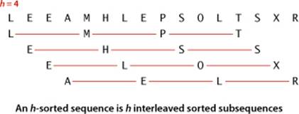
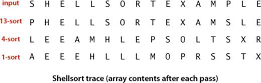
The idea is to rearrange the array to give it the property that taking every hth entry (starting anywhere) yields a sorted subsequence. Such an array is said to be h-sorted. Put another way, an h-sorted array is h independent sorted subsequences, interleaved together. By h-sorting for some large values of h, we can move items in the array long distances and thus make it easier to h-sort for smaller values of h. Using such a procedure for any sequence of values of h that ends in 1 will produce a sorted array: that is shellsort. The implementation in ALGORITHM 2.3 on the facing page uses the sequence of decreasing values ½(3k−1), starting at the smallest increment greater than or equal to N/3 and decreasing to 1. We refer to such a sequence as an increment sequence. ALGORITHM 2.3 computes its increment sequence; another alternative is to store an increment sequence in an array.
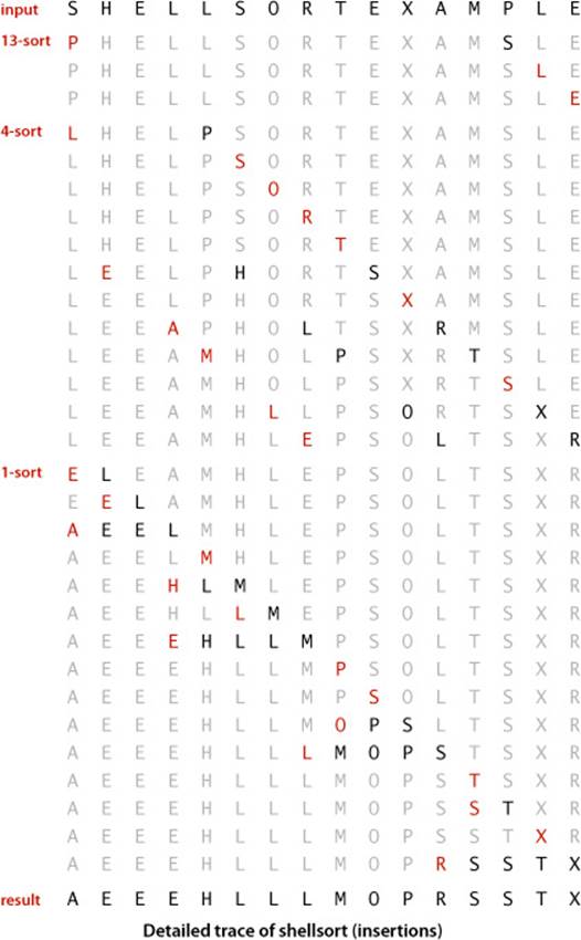
One way to implement shellsort would be, for each h, to use insertion sort independently on each of the h subsequences. Because the subsequences are independent, we can use an even simpler approach: when h-sorting the array, we insert each item among the previous items in its h-subsequence by exchanging it with those that have larger keys (moving them each one position to the right in the subsequence). We accomplish this task by using the insertion-sort code, but modified to decrement by h instead of 1 when moving through the array. This observation reduces the shellsort implementation to an insertion-sort-like pass through the array for each increment.
Shellsort gains efficiency by making a tradeoff between size and partial order in the subsequences. At the beginning, the subsequences are short; later in the sort, the subsequences are partially sorted. In both cases, insertion sort is the method of choice. The extent to which the subsequences are partially sorted is a variable factor that depends strongly on the increment sequence. Understanding shellsort’s performance is a challenge. Indeed, ALGORITHM 2.3 is the only sorting method we consider whose performance on randomly ordered arrays has not been precisely characterized.
Algorithm 2.3 Shellsort
public class Shell
{
public static void sort(Comparable[] a)
{ // Sort a[] into increasing order.
int N = a.length;
int h = 1;
while (h < N/3) h = 3*h + 1; // 1, 4, 13, 40, 121, 364, 1093, ...
while (h >= 1)
{ // h-sort the array.
for (int i = h; i < N; i++)
{ // Insert a[i] among a[i-h], a[i-2*h], a[i-3*h]... .
for (int j = i; j >= h && less(a[j], a[j-h]); j -= h)
exch(a, j, j-h);
}
h = h/3;
}
}
// See page 245 for less(), exch(), isSorted(), and main().
}
If we modify insertion sort (ALGORITHM 2.2) to h-sort the array and add an outer loop to decrease h through a sequence of increments starting at an increment as large as a constant fraction of the array length and ending at 1, we are led to this compact shellsort implementation.
% java SortCompare Shell Insertion 100000 100
For 100000 random Doubles
Shell is 600 times faster than Insertion
How do we decide what increment sequence to use? In general, this question is a difficult one to answer. The performance of the algorithm depends not just on the number of increments, but also on arithmetical interactions among the increments such as the size of their common divisors and other properties. Many different increment sequences have been studied in the literature, but no provably best sequence has been found. The increment sequence that is used in ALGORITHM 2.3 is easy to compute and use, and performs nearly as well as more sophisticated increment sequences that have been discovered that have provably better worst-case performance. Increment sequences that are substantially better still may be waiting to be discovered.
Shellsort is useful even for large arrays, particularly by contrast with selection sort and insertion sort. It also performs well on arrays that are in arbitrary order (not necessarily random). Indeed, constructing an array for which shellsort runs slowly for a particular increment sequence is usually a challenging exercise.
As you can learn with SortCompare, shellsort is much faster than insertion sort and selection sort, and its speed advantage increases with the array size. Before reading further, try using SortCompare to compare shellsort with insertion sort and selection sort for array sizes that are increasing powers of 2 on your computer (see EXERCISE 2.1.27). You will see that shellsort makes it possible to address sorting problems that could not be addressed with the more elementary algorithms. This example is our first practical illustration of an important principle that pervades this book: achieving speedups that enable the solution of problems that could not otherwise be solved is one of the prime reasons to study algorithm performance and design.
The study of the performance characteristics of shellsort requires mathematical arguments that are beyond the scope of this book. If you want to be convinced, start by thinking about how you would prove the following fact: when an h-sorted array is k-sorted, it remains h-sorted. As for the performance of ALGORITHM 2.3, the most important result in the present context is the knowledge that the running time of shellsort is not necessarily quadratic—for example, it is known that the worst-case number of compares for ALGORITHM 2.3 is proportional to N3/2. That such a simple modification can break the quadratic-running-time barrier is quite interesting, as doing so is a prime goal for many algorithm design problems.
No mathematical results are available about the average-case number of compares for shellsort for randomly ordered input. Increment sequences have been devised that drive the asymptotic growth of the worst-case number of compares down to N4/3, N5/4, N6/5, . . ., but many of these results are primarily of academic interest because these functions are hard to distinguish from one another (and from a constant factor of N) for practical values of N.
In practice, you can safely take advantage of the past scientific study of shellsort just by using the increment sequence in ALGORITHM 2.3 (or one of the increment sequences in the exercises at the end of this section, which may improve performance by 20 to 40 percent). Moreover, you can easily validate the following hypothesis:
Property E. The number of compares used by shellsort with the increments 1, 4, 13, 40, 121, 364, . . . is bounded by a small multiple of N times the number of increments used.
Evidence: Instrumenting ALGORITHM 2.3 to count compares and divide by the number of increments used is a straightforward exercise (see EXERCISE 2.1.12). Extensive experiments suggest that the average number of compares per increment might be N1/5, but it is quite difficult to discern the growth in that function unless N is huge. This property also seems to be rather insensitive to the input model.
EXPERIENCED PROGRAMMERS sometimes choose shellsort because it has acceptable running time even for moderately large arrays; it requires a small amount of code; and it uses no extra space. In the next few sections, we shall see methods that are more efficient, but they are perhaps only twice as fast (if that much) except for very large N, and they are more complicated. If you need a solution to a sorting problem, and are working in a situation where a system sort may not be available (for example, code destined for hardware or an embedded system), you can safely use shellsort, then determine sometime later whether it will be worthwhile to replace it with a more sophisticated method.
Q&A
Q. Sorting seems like a toy problem. Aren’t many of the other things that we do with computers much more interesting?
A. Perhaps, but many of those interesting things are made possible by fast sorting algorithms. You will find many examples in SECTION 2.5 and throughout the rest of the book. Sorting is worth studying now because the problem is easy to understand, and you can appreciate the ingenuity behind the faster algorithms.
Q. Why so many sorting algorithms?
A. One reason is that the performance of many algorithms depends on the input values, so different algorithms might be appropriate for different applications having different kinds of input. For example, insertion sort is the method of choice for partially sorted or tiny arrays. Other constraints, such as space and treatment of equal keys, also come into play. We will revisit this question in SECTION 2.5.
Q. Why bother using the tiny helper methods less() and exch()?
A. They are basic abstract operations needed by any sort algorithm, and the code is easier to understand in terms of these abstractions. Moreover, they make the code directly portable to other settings. For example, much of the code in ALGORITHMS 2.1 and 2.2 is legal code in several other programming languages. Even in Java, we can use this code as the basis for sorting primitive types (which are not Comparable): simply implement less() with the code v < w.
Q. When I run SortCompare, I get different values each time that I run it (and those are different from the values in the book). Why?
A. For starters, you have a different computer from the one we used, not to mention a different operating system, Java runtime, and so forth. All of these differences might lead to slight differences in the machine code for the algorithms. Differences each time that you run it on your computer might be due to other applications that you are running or various other conditions. Running a very large number of trials should dampen the effect. The lesson is that small differences in algorithm performance are difficult to notice nowadays. That is a primary reason that we focus on large ones!
Exercises
2.1.1 Show, in the style of the example trace with ALGORITHM 2.1, how selection sort sorts the array E A S Y Q U E S T I O N.
2.1.2 What is the maximum number of exchanges involving any particular item during selection sort? What is the average number of exchanges involving an item?
2.1.3 Give an example of an array of N items that maximizes the number of times the test a[j] < a[min] succeeds (and, therefore, min gets updated) during the operation of selection sort (ALGORITHM 2.1).
2.1.4 Show, in the style of the example trace with ALGORITHM 2.2, how insertion sort sorts the array E A S Y Q U E S T I O N.
2.1.5 For each of the two conditions in the inner for loop in insertion sort (ALGORITHM 2.2), describe an array of N items where that condition is always false when the loop terminates.
2.1.6 Which method runs faster for an array with all keys identical, selection sort or insertion sort?
2.1.7 Which method runs faster for an array in reverse order, selection sort or insertion sort?
2.1.8 Suppose that we use insertion sort on a randomly ordered array where items have only one of three values. Is the running time linear, quadratic, or something in between?
2.1.9 Show, in the style of the example trace with ALGORITHM 2.3, how shellsort sorts the array E A S Y S H E L L S O R T Q U E S T I O N.
2.1.10 Why not use selection sort for h-sorting in shellsort?
2.1.11 Implement a version of shellsort that keeps the increment sequence in an array, rather than computing it.
2.1.12 Instrument shellsort to print the number of compares divided by the array size for each increment. Write a test client that tests the hypothesis that this number is a small constant, by sorting arrays of random Double values, using array sizes that are increasing powers of 10, starting at 100.
Creative Problems
2.1.13 Deck sort. Explain how you would put a deck of cards in order by suit (in the order spades, hearts, clubs, diamonds) and by rank within each suit, with the restriction that the cards must be laid out face down in a row, and the only allowed operations are to check the values of two cards and to exchange two cards (keeping them face down).
2.1.14 Dequeue sort. Explain how you would sort a deck of cards, with the restriction that the only allowed operations are to look at the values of the top two cards, to exchange the top two cards, and to move the top card to the bottom of the deck.
2.1.15 Expensive exchange. A clerk at a shipping company is charged with the task of rearranging a number of large crates in order of the time they are to be shipped out. Thus, the cost of compares is very low (just look at the labels) relative to the cost of exchanges (move the crates). The warehouse is nearly full—there is extra space sufficient to hold any one of the crates, but not two. What sorting method should the clerk use?
2.1.16 Certification. Write a check() method that calls sort() for a given array and returns true if sort() puts the array in order and leaves the same set of objects in the array as were there initially, false otherwise. Do not assume that sort() is restricted to move data only with exch(). You may useArrays.sort() and assume that it is correct.
2.1.17 Animation. Add code to Insertion, Selection and Shell to make them draw the array contents as vertical bars like the visual traces in this section, redrawing the bars after each pass, to produce an animated effect, ending in a “sorted” picture where the bars appear in order of their height.Hint: Use a client like the one in the text that generates random Double values, insert calls to show() as appropriate in the sort code, and implement a show() method that clears the canvas and draws the bars.
2.1.18 Visual trace. Modify your solution to the previous exercise to make Insertion Selection and Shell produce visual traces such as those depicted in this section. Hint: Judicious use of setYscale() makes this problem easy. Extra credit: Add the code necessary to produce red and gray color accents such as those in our figures.
2.1.19 Shellsort worst case. Construct an array of 100 elements containing the numbers 1 through 100 for which shellsort, with the increments 1 4 13 40, uses as large a number of compares as you can find.
2.1.20 Shellsort best case. What is the best case for shellsort? Justify your answer.
2.1.21 Comparable transactions. Using our code for Date (page 247) as a model, expand your implementation of Transaction (EXERCISE 1.2.13) so that it implements Comparable, such that transactions are kept in order by amount.
Solution:
public class Transaction implements Comparable<Transaction>
{
...
private final double amount;
...
public int compareTo(Transaction that)
{
if (this.amount > that.amount) return +1;
if (this.amount < that.amount) return -1;
return 0;
}
...
}
2.1.22 Transaction sort test client. Write a class SortTransactions that consists of a static method main() that reads a sequence of transactions from standard input, sorts them, and prints the result on standard output (see EXERCISE 1.3.17).
Solution:
public class SortTransactions
{
public static Transaction[] readTransactions()
{ /* See Exercise 1.3.17 */ }
public static void main(String[] args)
{
Transaction[] transactions = readTransactions();
Shell.sort(transactions);
for (Transaction t : transactions)
StdOut.println(t);
}
}
Experiments
2.1.23 Deck sort. Ask a few friends to sort a deck of cards (see EXERCISE 2.1.13). Observe them carefully and write down the method(s) that they use.
2.1.24 Insertion sort with sentinel. Develop an implementation of insertion sort that eliminates the j>0 test in the inner loop by first putting the smallest item into position. Use SortCompare to evaluate the effectiveness of doing so. Note: It is often possible to avoid an index-out-of-bounds test in this way—the element that enables the test to be eliminated is known as a sentinel.
2.1.25 Insertion sort without exchanges. Develop an implementation of insertion sort that moves larger elements to the right one position with one array access per entry, rather than using exch(). Use SortCompare to evaluate the effectiveness of doing so.
2.1.26 Primitive types. Develop a version of insertion sort that sorts arrays of int values and compare its performance with the implementation given in the text (which sorts Integer values and implicitly uses autoboxing and auto-unboxing to convert).
2.1.27 Shellsort is subquadratic. Use SortCompare to compare shellsort with insertion sort and selection sort on your computer. Use array sizes that are increasing powers of 2, starting at 128.
2.1.28 Equal keys. Formulate and validate hypotheses about the running time of insertion sort and selection sort for arrays that contain just two key values, assuming that the values are equally likely to occur.
2.1.29 Shellsort increments. Run experiments to compare the increment sequence in ALGORITHM 2.3 with the sequence 1, 5, 19, 41, 109, 209, 505, 929, 2161, 3905, 8929, 16001, 36289, 64769, 146305, 260609 (which is formed by merging together the sequences 9·4k − 9·2k + 1 and 4k − 3·2k + 1). See EXERCISE 2.1.11.
2.1.30 Geometric increments. Run experiments to determine a value of t that leads to the lowest running time of shellsort for random arrays for the increment sequence 1, ![]() t
t![]() ,
, ![]() t2
t2![]() ,
, ![]() t3
t3![]() ,
, ![]() t4
t4![]() , . . . for N = 106. Give the values of t and the increment sequences for the best three values that you find.
, . . . for N = 106. Give the values of t and the increment sequences for the best three values that you find.
The following exercises describe various clients for helping to evaluate sorting methods. They are intended as starting points for helping to understand performance properties, using random data. In all of them, use time(), as in SortCompare, so that you can get more accurate results by specifying more trials in the second command-line argument. We refer back to these exercises in later sections when evaluating more sophisticated methods.
2.1.31 Doubling test. Write a client that performs a doubling test for sort algorithms. Start at N equal to 1000, and print N, the predicted number of seconds, the actual number of seconds, and the ratio as N doubles. Use your program to validate that insertion sort and selection sort are quadratic for random inputs, and formulate and test a hypothesis for shellsort.
2.1.32 Plot running times. Write a client that uses StdDraw to plot the average running times of the algorithm for random inputs and various values of the array size. You may add one or two more command-line arguments. Strive to design a useful tool.
2.1.33 Distribution. Write a client that enters into an infinite loop running sort() on arrays of the size given as the third command-line argument, measures the time taken for each run, and uses StdDraw to plot the average running times. A picture of the distribution of the running times should emerge.
2.1.34 Corner cases. Write a client that runs sort() on difficult or pathological cases that might turn up in practical applications. Examples include arrays that are already in order, arrays in reverse order, arrays where all keys are the same, arrays consisting of only two distinct values, and arrays of size 0 or 1.
2.1.35 Nonuniform distributions. Write a client that generates test data by randomly ordering objects using other distributions than uniform, including the following:
• Gaussian
• Poisson
• Geometric
• Discrete (see EXERCISE 2.1.28 for a special case)
Develop and test hypotheses about the effect of such input on the performance of the algorithms in this section.
2.1.36 Nonuniform data. Write a client that generates test data that is not uniform, including the following:
• Half the data is 0s, half 1s.
• Half the data is 0s, half the remainder is 1s, half the remainder is 2s, and so forth.
• Half the data is 0s, half random int values.
Develop and test hypotheses about the effect of such input on the performance of the algorithms in this section.
2.1.37 Partially sorted. Write a client that generates partially sorted arrays, including the following:
• 95 percent sorted, last percent random values
• All entries within 10 positions of their final place in the array
• Sorted except for 5 percent of the entries randomly dispersed throughout the array
Develop and test hypotheses about the effect of such input on the performance of the algorithms in this section.
2.1.38 Various types of items. Write a client that generates arrays of items of various types with random key values, including the following:
• String key (at least ten characters), one double value
• double key, ten String values (all at least ten characters)
• int key, one int[20] value
Develop and test hypotheses about the effect of such input on the performance of the algorithms in this section.
All materials on the site are licensed Creative Commons Attribution-Sharealike 3.0 Unported CC BY-SA 3.0 & GNU Free Documentation License (GFDL)
If you are the copyright holder of any material contained on our site and intend to remove it, please contact our site administrator for approval.
© 2016-2026 All site design rights belong to S.Y.A.