Algorithms (2014)
Four. Graphs
4.2 Directed Graphs
In directed graphs, edges are one-way: the pair of vertices that defines each edge is an ordered pair that specifies a one-way adjacency. Many applications (for example, graphs that represent the web, scheduling constraints, or telephone calls) are naturally expressed in terms of directed graphs. The one-way restriction is natural, easy to enforce in our implementations, and seems innocuous; but it implies added combinatorial structure that has profound implications for our algorithms and makes working with directed graphs quite different from working with undirected graphs. In this section, we consider classic algorithms for exploring and processing directed graphs.
Glossary
Our definitions for directed graphs are nearly identical to those for undirected graphs (as are some of the algorithms and programs that we use), but they are worth restating. The slight differences in the wording to account for edge directions imply structural properties that will be the focus of this section.
Definition. A directed graph (or digraph) is a set of vertices and a collection of directed edges. Each directed edge connects an ordered pair of vertices.
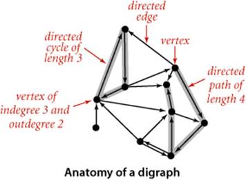
We say that a directed edge points from the first vertex in the pair and points to the second vertex in the pair. The outdegree of a vertex in a digraph is the number of edges pointing from it; the indegree of a vertex is the number of edges pointing to it. We drop the modifier directed when referring to edges in digraphs when the distinction is obvious in context. The first vertex in a directed edge is called its tail; the second vertex is called its head. We draw directed edges as arrows pointing from tail to head. We use the notation v->w to refer to an edge that points from v to w in a digraph. As with undirected graphs, our code handles parallel edges and self-loops, but they are not present in examples and we generally ignore them in the text. Ignoring anomalies, there are four different ways in which two vertices might be related in a digraph: no edge; an edge v->w from vto w; an edge w->v from w to v; or two edges v->w and w->v, which indicate connections in both directions.
Definition. A directed path in a digraph is a sequence of vertices in which there is a (directed) edge pointing from each vertex in the sequence to its successor in the sequence. A directed cycle is a directed path with at least one edge whose first and last vertices are the same. A simple path is a path with no repeated vertices. A simple cycle is a cycle with no repeated edges or vertices (except the requisite repetition of the first and last vertices). The length of a path or a cycle is its number of edges.
As for undirected graphs, we assume that directed paths are simple unless we specifically relax this assumption by referring to specific repeated vertices (as in our definition of directed cycle) or to general directed paths. We say that a vertex w is reachable from a vertex v if there is a directed path from v to w. Also, we adopt the convention that each vertex is reachable from itself. Except for this case, the fact that w is reachable from v in a digraph indicates nothing about whether v is reachable from w. This distinction is obvious, but critical, as we shall see.
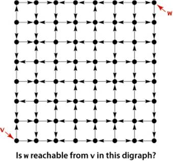
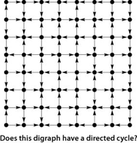
UNDERSTANDING THE ALGORITHMS in this section requires an appreciation of the distinction between reachability in digraphs and connectivity in undirected graphs. Developing such an appreciation is more complicated than you might think. For example, although you are likely to be able to tell at a glance whether two vertices in a small undirected graph are connected, a directed path in a digraph is not so easy to spot, as indicated in the example at left. Processing digraphs is akin to traveling around in a city where all the streets are one-way, with the directions not necessarily assigned in any uniform pattern. Getting from one point to another in such a situation could be a challenge indeed. Counter to this intuition is the fact that the standard data structure that we use for representing digraphs is simpler than the corresponding representation for undirected graphs!
Digraph data type
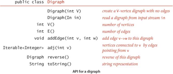
The API below and the class Digraph shown on the facing page are virtually identical to those for Graph (page 526).
Representation
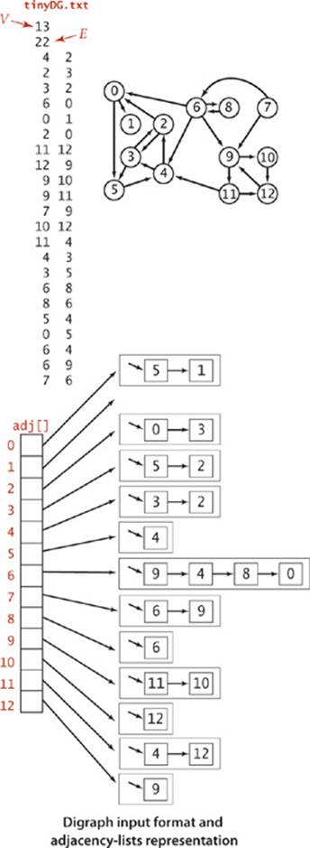
We use the adjacency-lists representation, where an edge v->w is represented as a list node containing w in the linked list corresponding to v. This representation is essentially the same as for undirected graphs but is even more straightforward because each edge occurs just once, as shown on the facing page.
Input format
The code for the constructor that takes a digraph from an input stream is identical to the corresponding constructor in Graph—the input format is the same, but all edges are interpreted to be directed edges. In the list-of-edges format, a pair v w is interpreted as an edge v->w.
Reversing a digraph
Digraph also adds to the API a method reverse() which returns a copy of the digraph, with all edges reversed. This method is sometimes needed in digraph processing because it allows clients to find the edges that point to each vertex, while adj() gives just vertices connected by edges that pointfrom each vertex.
Symbolic names
It is also a simple matter to allow clients to use symbolic names in digraph applications. To implement a class SymbolDigraph like SymbolGraph on page 552, replace Graph by Digraph everywhere.
IT IS WORTHWHILE to take the time to consider carefully the difference, by comparing code and the figure at right with their counterparts for undirected graphs on page 524 and page 526. In the adjacency-lists representation of an undirected graph, we know that if v is on w’s list, then w will be onv’s list; the adjacency-lists representation of a digraph has no such symmetry. This difference has profound implications in processing digraphs.
Directed graph (digraph) data type
public class Digraph
{
private final int V;
private int E;
private Bag<Integer>[] adj;
public Digraph(int V)
{
this.V = V;
this.E = 0;
adj = (Bag<Integer>[]) new Bag[V];
for (int v = 0; v < V; v++)
adj[v] = new Bag<Integer>();
}
public int V() { return V; }
public int E() { return E; }
public void addEdge(int v, int w)
{
adj[v].add(w);
E++;
}
public Iterable<Integer> adj(int v)
{ return adj[v]; }
public Digraph reverse()
{
Digraph R = new Digraph(V);
for (int v = 0; v < V; v++)
for (int w : adj(v))
R.addEdge(w, v);
return R;
}
}
This Digraph data type is identical to Graph (page 526) except that addEdge() only calls add() once, and it has an instance method reverse() that returns a copy with all its edges reversed. Since the code is easily derived from the corresponding code for Graph, we omit the toString() method (see the table on page 523) and the input stream constructor (see page 526).
Reachability in digraphs
Our first graph-processing algorithm for undirected graphs was DepthFirstSearch on page 531, which solves the single-source connectivity problem, allowing clients to determine which vertices are connected to a given source. The identical code with Graph changed to Digraph solves the analogous problem for digraphs:
Single-source reachability. Given a digraph and a source vertex s, support queries of the form Is there a directed path from s to a given target vertex v?
DirectedDFS on the facing page is a slight embellishment of DepthFirstSearch that implements the following API:
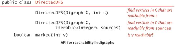
By adding a second constructor that takes a list of vertices, this API supports for clients the following generalization of the problem:
Multiple-source reachability. Given a digraph and a set of source vertices, support queries of the form Is there a directed path from some vertex in the set to a given target vertex v?
This problem arises in the solution of a classic string-processing problem that we consider in SECTION 5.4.
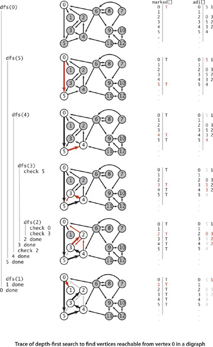
DirectedDFS uses our standard graph-processing paradigm and a standard recursive depth-first search to solve these problems. It calls the recursive dfs() for each source, which marks every vertex encountered.
Proposition D. DFS marks all the vertices in a digraph reachable from a given set of sources in time proportional to the sum of the outdegrees of the vertices marked.
Proof: Same as PROPOSITION A on page 531.
A trace of the operation of this algorithm for our sample digraph appears on page 572. This trace is somewhat simpler than the corresponding trace for undirected graphs, because DFS is fundamentally a digraph-processing algorithm, with one representation of each edge. Following this trace is a worthwhile way to help cement your understanding of depth-first search in digraphs.
Algorithm 4.4 Reachability in digraphs
public class DirectedDFS
{
private boolean[] marked;
public DirectedDFS(Digraph G, int s)
{
marked = new boolean[G.V()];
dfs(G, s);
}
public DirectedDFS(Digraph G, Iterable<Integer> sources)
{
marked = new boolean[G.V()];
for (int s : sources)
if (!marked[s]) dfs(G, s);
}
private void dfs(Digraph G, int v)
{
marked[v] = true;
for (int w : G.adj(v))
if (!marked[w]) dfs(G, w);
}
public boolean marked(int v)
{ return marked[v]; }
public static void main(String[] args)
{
Digraph G = new Digraph(new In(args[0]));
Bag<Integer> sources = new Bag<Integer>();
for (int i = 1; i < args.length; i++)
sources.add(Integer.parseInt(args[i]));
DirectedDFS reachable = new DirectedDFS(G, sources);
for (int v = 0; v < G.V(); v++)
if (reachable.marked(v)) StdOut.print(v + " ");
StdOut.println();
}
}
% java DirectedDFS tinyDG.txt 1
1
% java DirectedDFS tinyDG.txt 2
0 1 2 3 4 5
% java DirectedDFS tinyDG.txt 1 2 6
0 1 2 3 4 5 6 8 9 10 11 12
This implementation of depth-first search provides clients the ability to test which vertices are reachable from a given vertex or a given set of vertices.
Mark-and-sweep garbage collection
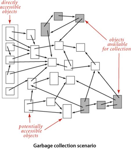
An important application of multiple-source reachability is found in typical memory-management systems, including many implementations of Java. A digraph where each vertex represents an object and each edge represents a reference to an object is an appropriate model for the memory usage of a running Java program. At any point in the execution of a program, certain objects are known to be directly accessible, and any object not reachable from that set of objects can be returned to available memory. A mark-and-sweep garbage collection strategy reserves one bit per object for the purpose of garbage collection, then periodically marks the set of potentially accessible objects by running a digraph reachability algorithm like DirectedDFS and sweeps through all objects, collecting the unmarked ones for use for new objects.
Finding paths in digraphs
DepthFirstPaths (ALGORITHM 4.1 on page 536) and BreadthFirstPaths (ALGORITHM 4.2 on page 540) are also fundamentally digraph-processing algorithms. Again, the identical APIs and code (with Graph changed to Digraph) effectively solve the following problems:
Single-source directed paths. Given a digraph and a source vertex s, support queries of the form Is there a directed path from s to a given target vertex v? If so, find such a path.
Single-source shortest directed paths. Given a digraph and a source vertex s, support queries of the form Is there a directed path from s to a given target vertex v? If so, find a shortest such path (one with a minimal number of edges).
On the booksite and in the exercises at the end of this section, we refer to these solutions as DepthFirstDirectedPaths and BreadthFirstDirectedPaths, respectively.
Cycles and DAGs
Directed cycles are of particular importance in applications that involve processing digraphs. Identifying directed cycles in a typical digraph can be a challenge without the help of a computer, as shown at right. In principle, a digraph might have a huge number of cycles; in practice, we typically focus on a small number of them, or simply are interested in knowing that none are present.
To motivate the study of the role of directed cycles in digraph processing we consider, as a running example, the following prototypical application where digraph models arise directly:
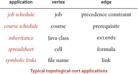
Scheduling problems
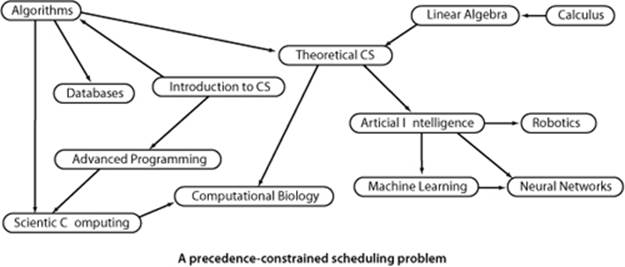
A widely applicable problem-solving model has to do with arranging for the completion of a set of jobs, under a set of constraints, by specifying when and how the jobs are to be performed. Constraints might involve functions of the time taken or other resources consumed by the jobs. The most important type of constraints is precedence constraints, which specify that certain jobs must be performed before certain others. Different types of additional constraints lead to many different types of scheduling problems, of varying difficulty. Literally thousands of different problems have been studied, and researchers still seek better algorithms for many of them. As an example, consider a college student planning a course schedule, under the constraint that certain courses are prerequisite for certain other courses, as in the example below.
If we further assume that the student can take only one course at a time, we have an instance of the following problem:
Precedence-constrained scheduling. Given a set of jobs to be completed, with precedence constraints that specify that certain jobs have to be completed before certain other jobs are begun, how can we schedule the jobs such that they are all completed while still respecting the constraints?
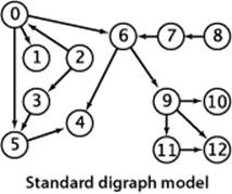
For any such problem, a digraph model is immediate, with vertices corresponding to jobs and directed edges corresponding to precedence constraints. For economy, we switch the example to our standard model with vertices labeled as integers, as shown at left. In digraphs, precedence-constrained scheduling amounts to the following fundamental problem:
Topological sort. Given a digraph, put the vertices in order such that all its directed edges point from a vertex earlier in the order to a vertex later in the order (or report that doing so is not possible).
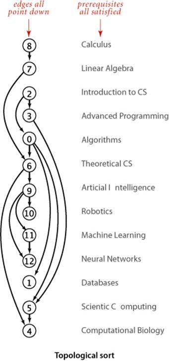
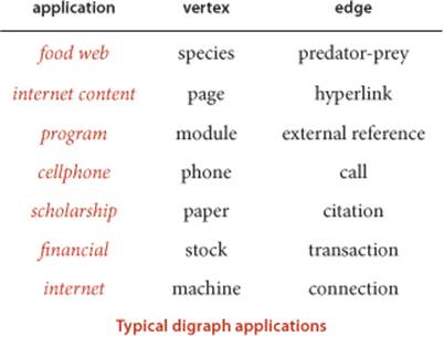
A topological order for our example model is shown at right. All edges point down, so it clearly represents a solution to the precedence-constrained scheduling problem that this digraph models: the student can satisfy all course prerequisites by taking the courses in this order. This application is typical—some other representative applications are listed in the table below.
Cycles in digraphs
If job x must be completed before job y, job y before job z, and job z before job x, then someone has made a mistake, because those three constraints cannot all be satisfied. In general, if a precedence-constrained scheduling problem has a directed cycle, then there is no feasible solution. To check for such errors, we need to be able to solve the following problem:
Directed cycle detection. Does a given digraph have a directed cycle? If so, find the vertices on some such cycle, in order from some vertex back to itself.
A graph may have an exponential number of cycles (see EXERCISE 4.2.11) so we only ask for one cycle, not all of them. For job scheduling and many other applications it is required that no directed cycle exists, so digraphs where they are absent play a special role:
Definition. A directed acyclic graph (DAG) is a digraph with no directed cycles.
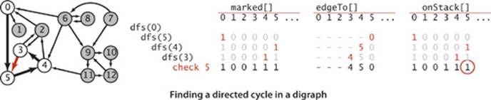
Solving the directed cycle detection problem thus answers the following question: Is a given digraph a DAG? Developing a depth-first-search-based solution to this problem is not difficult, based on the fact that the recursive call stack maintained by the system represents the “current” directed path under consideration (like the string back to the entrance in Tremaux maze exploration). If we ever find a directed edge v->w to a vertex w that is on that stack, we have found a cycle, since the stack is evidence of a directed path from w to v, and the edge v->w completes the cycle. Moreover, the absence of any such back edges implies that the graph is acyclic. DirectedCycle on the facing page uses this idea to implement the following API:
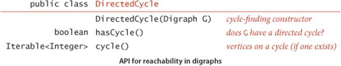
Finding a directed cycle
public class DirectedCycle
{
private boolean[] marked;
private int[] edgeTo;
private Stack<Integer> cycle; // vertices on a cycle (if one exists)
private boolean[] onStack; // vertices on recursive call stack
public DirectedCycle(Digraph G)
{
onStack = new boolean[G.V()];
edgeTo = new int[G.V()];
marked = new boolean[G.V()];
for (int v = 0; v < G.V(); v++)
if (!marked[v]) dfs(G, v);
}
private void dfs(Digraph G, int v)
{
onStack[v] = true;
marked[v] = true;
for (int w : G.adj(v))
if (this.hasCycle()) return;
else if (!marked[w])
{ edgeTo[w] = v; dfs(G, w); }
else if (onStack[w])
{
cycle = new Stack<Integer>();
for (int x = v; x != w; x = edgeTo[x])
cycle.push(x);
cycle.push(w);
cycle.push(v);
}
onStack[v] = false;
}
public boolean hasCycle()
{ return cycle != null; }
public Iterable<Integer> cycle()
{ return cycle; }
}
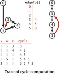
This class adds to our standard recursive dfs() a boolean array onStack[] to keep track of the vertices for which the recursive call has not completed. When it finds an edge v->w to a vertex w that is on the stack, it has discovered a directed cycle, which it can recover by following edgeTo[] links.
When executing dfs(G, v), we have followed a directed path from the source to v. To keep track of this path, DirectedCycle maintains a vertex-indexed array onStack[] that marks the vertices on the recursive call stack (by setting onStack[v] to true on entry to dfs(G, v) and to false on exit). DirectedCycle also maintains an edgeTo[] array so that it can return the cycle when it is detected, in the same way as DepthFirstPaths (page 536) and BreadthFirstPaths (page 540) return paths.
Depth-first orders and topological sort
Precedence-constrained scheduling amounts to computing a topological order for the vertices of a DAG, as in this API:
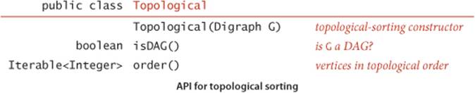
Proposition E. A digraph has a topological order if and only if it is a DAG.
Proof: If the digraph has a directed cycle, it has no topological order. Conversely, the algorithm that we are about to examine computes a topological order for any given DAG.
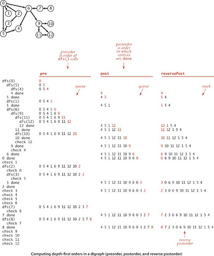
Remarkably, it turns out that we have already seen an algorithm for topological sort: a one-line addition to our standard recursive DFS does the job! To convince you of this fact, we begin with the class DepthFirstOrder on page 580. It is based on the idea that depth-first search visits each vertex exactly once. If we save the vertex given as argument to the recursive dfs() in a data structure, then iterate through that data structure, we see all the graph vertices, in order determined by the nature of the data structure and by whether we do the save before or after the recursive calls. Three vertex orderings are of interest in typical applications:
• Preorder: Put the vertex on a queue before the recursive calls.
• Postorder: Put the vertex on a queue after the recursive calls.
• Reverse postorder: Put the vertex on a stack after the recursive calls.
A trace of DepthFirstOrder for our sample DAG is given on the facing page. It is simple to implement and supports pre(), post(), and reversePost() methods that are useful for advanced graph-processing algorithms. For example, order() in Topological consists of a call on reversePost().
Depth-first search vertex ordering in a digraph
public class DepthFirstOrder
{
private boolean[] marked;
private Queue<Integer> pre; // vertices in preorder
private Queue<Integer> post; // vertices in postorder
private Stack<Integer> reversePost; // vertices in reverse postorder
public DepthFirstOrder(Digraph G)
{
pre = new Queue<Integer>();
post = new Queue<Integer>();
reversePost = new Stack<Integer>();
marked = new boolean[G.V()];
for (int v = 0; v < G.V(); v++)
if (!marked[v]) dfs(G, v);
}
private void dfs(Digraph G, int v)
{
pre.enqueue(v);
marked[v] = true;
for (int w : G.adj(v))
if (!marked[w])
dfs(G, w);
post.enqueue(v);
reversePost.push(v);
}
public Iterable<Integer> pre()
{ return pre; }
public Iterable<Integer> post()
{ return post; }
public Iterable<Integer> reversePost()
{ return reversePost; }
}
This class enables clients to iterate through the vertices in various orders defined by depth-first search. This ability is very useful in the development of advanced digraph-processing algorithms, because the recursive nature of the search enables us to prove properties of the computation (see, for example, PROPOSITION F).
Algorithm 4.5 Topological sort
public class Topological
{
private Iterable<Integer> order; // topological order
public Topological(Digraph G)
{
DirectedCycle cyclefinder = new DirectedCycle(G);
if (!cyclefinder.hasCycle())
{
DepthFirstOrder dfs = new DepthFirstOrder(G);
order = dfs.reversePost();
}
}
public Iterable<Integer> order()
{ return order; }
public boolean isDAG()
{ return order != null; }
public static void main(String[] args)
{
String filename = args[0];
String separator = args[1];
SymbolDigraph sg = new SymbolDigraph(filename, separator);
Topological top = new Topological(sg.G());
for (int v : top.order())
StdOut.println(sg.name(v));
}
}
This DepthFirstOrder and DirectedCycle client returns a topological order for a DAG. The test client solves the precedence-constrained scheduling problem for a SymbolDigraph. The instance method order() returns null if the given digraph is not a DAG and an iterator giving the vertices in topological order otherwise. The code for SymbolDigraph is omitted because it is precisely the same as for SymbolGraph (page 552), with Digraph replacing Graph everywhere.
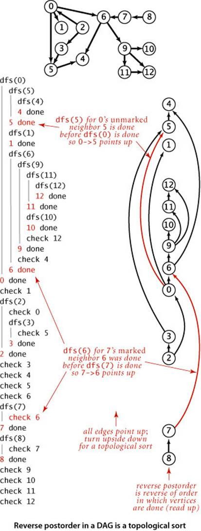
Proposition F. Reverse postorder in a DAG is a topological sort.
Proof: Consider any edge v->w. One of the following three cases must hold when dfs(v) is called (see the diagram on page 583):
• dfs(w) has already been called and has returned (w is marked).
• dfs(w) has not yet been called (w is unmarked), so v->w will cause dfs(w) to be called (and return), either directly or indirectly, before dfs(v) returns.
• dfs(w) has been called and has not yet returned when dfs(v) is called. The key to the proof is that this case is impossible in a DAG, because the recursive call chain implies a path from w to v and v->w would complete a directed cycle.
In the two possible cases, dfs(w) is done before dfs(v), so w appears before v in postorder and after v in reverse postorder. Thus, each edge v->w points from a vertex earlier in the order to a vertex later in the order, as desired.
% more jobs.txt
Algorithms/Theoretical CS/Databases/Scientific Computing
Introduction to CS/Advanced Programming/Algorithms
Advanced Programming/Scientific Computing
Scientific Computing/Computational Biology
Theoretical CS/Computational Biology/Artificial Intelligence
Linear Algebra/Theoretical CS
Calculus/Linear Algebra
Artificial Intelligence/Neural Networks/Robotics/Machine Learning
Machine Learning/Neural Networks
% java Topological jobs.txt "/"
Calculus
Linear Algebra
Introduction to CS
Advanced Programming
Algorithms
Theoretical CS
Artificial Intelligence
Robotics
Machine Learning
Neural Networks
Databases
Scientific Computing
Computational Biology
Topological (ALGORITHM 4.5 on page 581) is an implementation that uses depth-first search to topologically sort a DAG. A trace is given at right.
Proposition G. With DFS, we can topologically sort a DAG in time proportional to V+E.
Proof: Immediate from the code. It uses one depth-first search to ensure that the graph has no directed cycles, and another to do the reverse postorder ordering. Both involve examining all the edges and all the vertices, and thus take time proportional to V+E.
Despite the simplicity of this algorithm, it escaped attention for many years, in favor of a more intuitive algorithm based on maintaining a queue of vertices of indegree 0 (see EXERCISE 4.2.39).
IN PRACTICE, topological sorting and cycle detection go hand in hand, with cycle detection playing the role of a debugging tool. For example, in a job-scheduling application, a directed cycle in the underlying digraph represents a mistake that must be corrected, no matter how the schedule was formulated. Thus, a job-scheduling application is typically a three-step process:
• Specify the tasks and precedence constraints.
• Make sure that a feasible solution exists, by detecting and removing cycles in the underlying digraph until none exist.
• Solve the scheduling problem, using topological sort.
Similarly, any changes in the schedule can be checked for cycles (using DirectedCycle), then a new schedule computed (using Topological).
Strong connectivity in digraphs
We have been careful to maintain a distinction between reachability in digraphs and connectivity in undirected graphs. In an undirected graph, two vertices v and w are connected if there is a path connecting them—we can use that path to get from v to w or to get from w to v. In a digraph, by contrast, a vertex w is reachable from a vertex v if there is a directed path from v to w, but there may or may not be a directed path back to v from w. To complete our study of digraphs, we consider the natural analog of connectivity in undirected graphs.
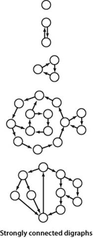
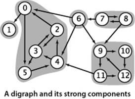
Definition. Two vertices v and w are strongly connected if they are mutually reachable: that is, if there is a directed path from v to w and a directed path from w to v. A digraph is strongly connected if all its vertices are strongly connected to one another.
Several examples of strongly connected graphs are given in the figure at left. As you can see from the examples, cycles play an important role in understanding strong connectivity. Indeed, recalling that a general directed cycle is a directed cycle that may have repeated vertices, it is easy to see that two vertices are strongly connected if and only if there exists a general directed cycle that contains them both. (Proof: compose the paths from v to w and from w to v.)
Strong components
Like connectivity in undirected graphs, strong connectivity in digraphs is an equivalence relation on the set of vertices, as it has the following properties:
• Reflexive: Every vertex v is strongly connected to itself.
• Symmetric: If v is strongly connected to w, then w is strongly connected to v.
• Transitive: If v is strongly connected to w and w is strongly connected to x, then v is also strongly connected to x.
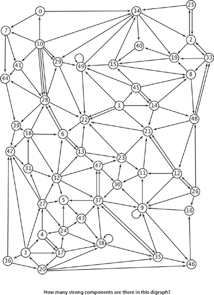
As an equivalence relation, strong connectivity partitions the vertices into equivalence classes. The equivalence classes are maximal subsets of vertices that are strongly connected to one another, with each vertex in exactly one subset. We refer to these subsets as strongly connected components, or strong components for short. Our sample digraph tinyDG.txt has five strong components, as shown in the diagram at right. A digraph with V vertices has between 1 and V strong components—a strongly connected digraph has 1 strong component and a DAG has V strong components. Note that the strong components are defined in terms of the vertices, not the edges. Some edges connect two vertices in the same strong component; some other edges connect vertices in different strong components. The latter are not found on any directed cycle. Just as identifying connected components is typically important in processing undirected graphs, identifying strong components is typically important in processing digraphs.
Examples of applications
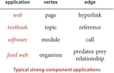
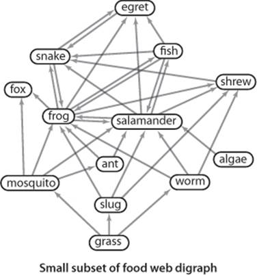
Strong connectivity is a useful abstraction in understanding the structure of a digraph, highlighting interrelated sets of vertices (strong components). For example, strong components can help textbook authors decide which topics should be grouped together and software developers decide how to organize program modules. The figure below shows an example from ecology. It illustrates a digraph that models the food web connecting living organisms, where vertices represent species and an edge from one vertex to another indicates that an organism of the species indicated by the point to vertex consumes organisms of the species indicated by the point to vertex for food. Scientific studies on such digraphs (with carefully chosen sets of species and carefully documented relationships) play an important role in helping ecologists answer basic questions about ecological systems. Strong components in such digraphs can help ecologists understand energy flow in the food web. The figure on page 591 shows a digraph model of web content, where vertices represent pages and edges represent hyperlinks from one page to another. Strong components in such a digraph can help network engineers partition the huge number of pages on the web into more manageable sizes for processing. Further properties of these applications and other examples are addressed in the exercises and on the booksite.
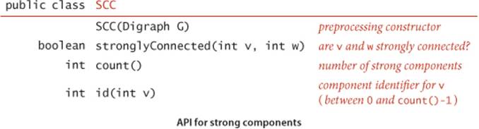
Accordingly, we need the following API, the analog for digraphs of CC (page 543):
A quadratic algorithm to compute strong components is not difficult to develop (see EXERCISE 4.2.31), but (as usual) quadratic time and space requirements are prohibitive for huge digraphs that arise in practical applications like the ones just described.
Kosaraju–Sharir algorithm.
We saw in CC (ALGORITHM 4.3 on page 544) that computing connected components in undirected graphs is a simple application of depth-first search. How can we efficiently compute strong components in digraphs? Remarkably, the implementation KosarajuSharirSCC on the facing page does the job with just a few lines of code added to CC, as follows:
• Given a digraph G, use DepthFirstOrder to compute the reverse postorder of its reverse digraph, GR.
• Run standard DFS on G, but consider the unmarked vertices in the order just computed instead of the standard numerical order.
• All vertices visited on a call to the recursive dfs() from the constructor are a strong component (!), so identify them as such, in the same manner as in CC.
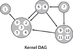
The Kosaraju–Sharir algorithm is an extreme example of a method that is easy to code but difficult to understand. To persuade yourself that the algorithm is correct, start by considering the kernel DAG (or condensation digraph) associated with each digraph, formed by collapsing all the vertices in each strong component to a single vertex (and removing any self-loops). The result must be a DAG because any directed cycle would imply a larger strong component. The kernel DAG for the digraph on page 584 has five vertices and seven edges, as shown at right (note the possibility of parallel edges). Since the kernel DAG is a DAG, its vertices can be placed in (reverse) topological order, as shown in the diagram at the top of page 588. This ordering is the key to understanding the Kosaraju–Sharir algorithm.
Algorithm 4.6 Kosaraju–Sharir algorithm for computing strong components
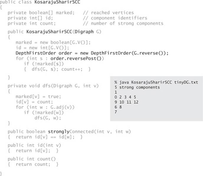
This implementation differs from CC (ALGORITHM 4.3) only in the highlighted code (and in the implementation of main() where we use the code on page 543, with Graph changed to Digraph, CC changed to KosarajuSharirSCC, and “components” changed to “strong components”). To find strong components, it does a depth-first search in the reverse digraph to produce a vertex order (reverse postorder of that search) for use in a depth-first search of the given digraph.
The Kosaraju-Sharir algorithm identifies the strong components in reverse topological order of the kernel DAG. It begins by finding a vertex that is in a sink component of the kernel DAG. When it runs DFS from that vertex, it visits precisely the vertices in that component. The DFS marks those vertices, effectively removing them from the digraph. Next, it finds a vertex that is in a sink component in the remaining kernel DAG, visits precisely the vertices in that component, and so forth.
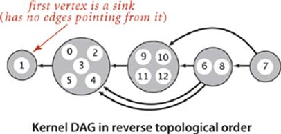
The postorder of GR enables us to examine the strong components in the desired order. The first vertex in a reverse postorder of G is in a source component of the kernel DAG; the first vertex in a reverse postorder of the reverse digraph GR is in a sink component of the kernel DAG (seeEXERCISE 4.2.16). More generally, the following lemma relates the reverse postorder of GR to the strong components, based on edges in the kernel DAG: it is the key to establishing the correctness of the Kosaraju–Sharir algorithm.
Postorder lemma. Let C be a strong component in a digraph G and let v be any vertex not in C. If there is an edge e pointing from any vertex in C to v, then vertex v appears before every vertex in C in the reverse postorder of GR.
Proof: See EXERCISE 4.2.15.
Proposition H. The Kosaraju—Sharir algorithm identifies the strong components of a digraph G.
Proof: By induction on the number of strong components identified in the DFS of G. After the algorithm has identified the first i components, we assume (by our inductive hypothesis) that the vertices in the first i components are marked and the vertices in the remaining components are unmarked. Let s be the unmarked vertex that appears first in the reverse postorder of GR. Then, the constructor call dfs(G, s) will visit every vertex in the strong component containing s (which we refer to as component i+1) and only those vertices because:
• Vertices in the first i components will not be visited (because they are already marked).
• Vertices in component i+1 are not yet marked and are reachable from s using only other vertices in component i+1 (so will be visited and marked).
• Vertices in components after i+1 will not be visited (or marked): Consider (for the sake of contradiction) the first such vertex v that is visited. Let e be an edge that goes from a vertex in component i+1 to v. By the postorder lemma, v appears in the reverse postorder before every vertex in component i+1 (including s). This contradicts the definition of s.
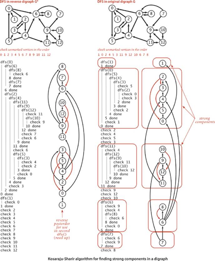
A trace of the algorithm for tinyDG.txt is shown on the preceding page. To the right of each DFS trace is a drawing of the digraph, with vertices appearing in the order they are done. Thus, reading up the reverse digraph drawing on the left gives the reverse postorder in GR, the order in which unmarked vertices are checked in the DFS of G. As you can see from the diagram, the second DFS calls dfs(1) (which marks vertex 1) then calls dfs(0) (which marks 0, 5, 4, 3, and 2), then checks 2, 4, 5, and 3, then calls dfs(11) (which marks 11, 12, 9, and 10), then checks 9, 12, and 10, then callsdfs(6) (which marks 6 and 8), and finally dfs(7), which marks 7.
A larger example, a very small subset of a digraph model of the web, is shown on the facing page.
THE KOSARAJU–SHARIR ALGORITHM solves the following analog of the connectivity problem for undirected graphs that we first posed in CHAPTER 1 and reintroduced in SECTION 4.1 (page 534):
Strong connectivity. Given a digraph, support queries of the form: Are two given vertices strongly connected? and How many strong components does the digraph have?
That we can solve this problem in digraphs as efficiently as the corresponding connectivity problem in undirected graphs was an open research problem for some time (resolved by R. E. Tarjan in the early 1970s). That such a simple solution is now available is quite surprising.
Proposition I. The Kosaraju–Sharir algorithm uses preprocessing time and space proportional to V+E to support constant-time strong connectivity queries in a digraph.
Proof: The algorithm computes the reverse of the digraph and does two depth-first searches. Each of these three steps takes time proportional to V+E. The reverse copy of the digraph uses space proportional to V+E.
Reachability revisited
With CC for undirected graphs, we can infer from the fact that two vertices v and w are connected that there is a path from v to w and a path (the same one) from w to v. With KosarajuSharirSCC, we can infer from the fact that v and w are strongly connected that there is a path from v to w and a path (a different one) from w to v. But what about pairs of vertices that are not strongly connected? There may be a path from v to w or a path from w to v or neither, but not both.
All-pairs reachability. Given a digraph, support queries of the form Is there a directed path from a given vertex v to another given vertex w?
For undirected graphs, the corresponding problem is equivalent to the connectivity problem; for digraphs, it is quite different from the strong connectivity problem. Our CC implementation uses linear preprocessing time to support constant-time answers to such queries for undirected graphs. Can we achieve this performance for digraphs? This seemingly innocuous question has confounded experts for decades. To better understand the challenge, consider the diagram at left, which illustrates the following fundamental concept:
Definition. The transitive closure of a digraph G is another digraph with the same set of vertices, but with an edge from v to w in the transitive closure if and only if w is reachable from v in G.
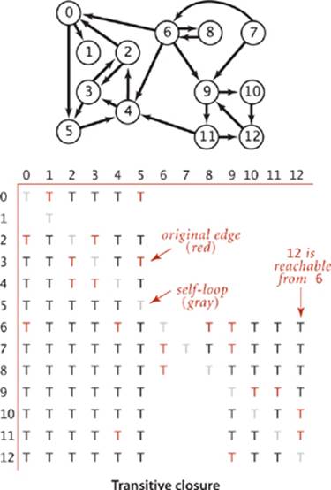
By convention, every vertex is reachable from itself, so the transitive closure has V self-loops. Our sample digraph has just 22 directed edges, but its transitive closure has 108 out of a possible 169 directed edges. Generally, the transitive closure of a digraph has many more edges than the digraph itself, and it is not at all unusual for a sparse graph to have a dense transitive closure. For example, the transitive closure of a V-vertex directed cycle, which has V directed edges, is a complete digraph with V2 directed edges. Since transitive closures are typically dense, we normally represent them with a matrix of boolean values, where the entry in row v and column w is true if and only if w is reachable from v. Instead of explicitly computing the transitive closure, we use depth-first search to implement the following API:
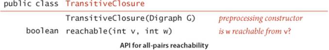
The code below is a straightforward implementation that uses DirectedDFS (ALGORITHM 4.4). This solution is ideal for small or dense digraphs, but it is not a solution for the large digraphs we might encounter in practice because the constructor uses space proportional to V2 and time proportional to V (V+E): each of the V DirectedDFS objects takes space proportional to V (they all have marked[] arrays of size V and examine E edges to compute the marks). Essentially, TransitiveClosure computes and stores the transitive closure of G, to support constant-time queries—row v in the transitive closure matrix is the marked[] array for the vth entry in the DirectedDFS[] in TransitiveClosure. Can we support constant-time queries with substantially less preprocessing time and substantially less space? A general solution that achieves constant-time queries with substantially less than quadratic space is an unsolved research problem, with important practical implications: for example, until it is solved, we cannot hope to have a practical solution to the all-pairs reachability problem for a giant digraph such as the web graph.
All-pairs reachability
public class TransitiveClosure
{
private DirectedDFS[] all;
TransitiveClosure(Digraph G)
{
all = new DirectedDFS[G.V()];
for (int v = 0; v < G.V(); v++)
all[v] = new DirectedDFS(G, v);
}
boolean reachable(int v, int w)
{ return all[v].marked(w); }
}
Summary
In this section, we have introduced directed edges and digraphs, emphasizing the relationship between digraph processing and corresponding problems for undirected graphs, as summarized in the following list of topics:
• Digraph nomenclature
• The idea that the representation and approach are essentially the same as for undirected graphs, but some digraph problems are more complicated
• Cycles, DAGs, topological sort, and precedence-constrainted scheduling
• Reachability, paths, and strong connectivity in digraphs
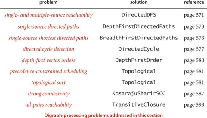
The table below summarizes the implementations of digraph algorithms that we have considered (all but one of the algorithms are based on depth-first search). The problems addressed are all simply stated, but the solutions that we have considered range from easy adaptations of corresponding algorithms for undirected graphs to an ingenious and surprising solution. These algorithms are a starting point for several of the more complicated algorithms that we consider in SECTION 4.4, when we consider edge-weighted digraphs.
Q&A
Q. Is a self-loop a cycle?
A. Yes, but no self-loop is needed for a vertex to be reachable from itself.
Exercises
4.2.1 What is the maximum number of edges in a digraph with V vertices and no parallel edges? What is the minimum number of edges in a digraph with V vertices, none of which are isolated?
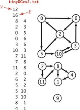
4.2.2 Draw, in the style of the figure in the text (page 524), the adjacency lists built by Digraph’s input stream constructor for the file tinyDGex2.txt depicted at left.
4.2.3 Create a copy constructor for Digraph that takes as input a digraph G and creates and initializes a new copy of the digraph. Any changes a client makes to G should not affect the newly created digraph.
4.2.4 Add a method hasEdge() to Digraph which takes two int arguments v and w and returns true if the graph has an edge v->w, false otherwise.
4.2.5 Modify Digraph to disallow parallel edges and self-loops.
4.2.6 Develop a test client for Digraph.
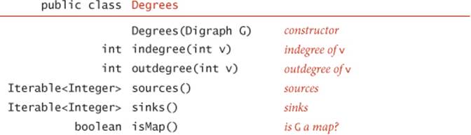
4.2.7 The indegree of a vertex in a digraph is the number of directed edges that point to that vertex. The outdegree of a vertex in a digraph is the number of directed edges that emanate from that vertex. No vertex is reachable from a vertex of outdegree 0, which is called a sink; a vertex of indegree 0, which is called a source, is not reachable from any other vertex. A digraph where self-loops are allowed and every vertex has outdegree 1 is called a map (a function from the set of integers from 0 to V–1 onto itself). Write a program Degrees.java that implements the following API:
4.2.8 Draw all the nonisomorphic DAGs with two, three, four, and five vertices (see EXERCISE 4.1.28).
4.2.9 Write a method that checks whether a given permutation of a DAG’s vertices is a topological order of that DAG.
4.2.10 Given a DAG, does there exist a topological order that cannot result from applying a DFS-based algorithm, no matter in what order the vertices adjacent to each vertex are chosen? Prove your answer.
4.2.11 Describe a family of sparse digraphs whose number of directed cycles grows exponentially in the number of vertices.
4.2.12 Prove that the strong components in GR are the same as in G.
4.2.13 Prove that two vertices in a digraph G are in the same strong component if and only if there is a directed cycle (not necessarily simple) containing both of them.
4.2.14 Let C be a strong component in a digraph G and let v be any vertex not in C. Prove that if there is an edge e pointing from v to any vertex in C, then vertex v appears before every vertex in C in the reverse postorder of G.
Solution: If v is visited before every vertex in C, then every vertex in C will be visited and finished before v finishes (because every vertex in C is reachable from v via edge e). If some vertex in C is visited before v, then all vertices in C will be visited and finished before v is visited (because vis not reachable from any vertex in C—if it were, such a path when combined with edge e would be part of a directed cycle, implying that v is in C).
4.2.15 Let C be a strong component in a digraph G and let v be any vertex not in C. Prove that if there is an edge e pointing from any vertex in C to v, then vertex v appears before every vertex in C in the reverse postorder of GR.
Solution: Apply EXERCISE 4.2.14 to GR.
4.2.16 Given a digraph G, prove that the first vertex in the reverse postorder of G is in a strong component that is a source of G’s kernel DAG. Then, prove that the first vertex in the reverse postorder of GR is in a strong component that is a sink of G’s kernel DAG.
Hint: Apply EXERCISES 4.2.14 and 4.2.15.
4.2.17 How many strong components are there in the digraph on page 591?
4.2.18 What are the strong components of a DAG?.
Creative Problems
4.2.19 What happens if you run the Kosaraju–Sharir algorithm on a DAG?
4.2.20 True or false: The reverse postorder of a digraph's reverse is the same as the postorder of the digraph.
4.2.21 True or false: If we consider the vertices of a digraph G (or its reverse GR) in postorder, then vertices in the same strong component will be consecutive in that order.
Solution : False. In tinyDG.txt, vertices 6 and 8 form a strong component, but they are not consecutive in the postorder of GR.
4.2.22 True or false: If we modify the Kosaraju–Sharir algorithm to run the first depth-first search in the digraph G (instead of the reverse digraph GR) and the second depth-first search in GR (instead of G), then it will still find the strong components.
4.2.23 True or false: If we modify the Kosaraju–Sharir algorithm to replace the second depth-first search with breadth-first search, then it will still find the strong components.
4.2.24 Compute the memory usage of a Digraph with V vertices and E edges, under the memory cost model of SECTION 1.4.
4.2.25 How many edges are there in the transitive closure of a digraph that is a simple directed path with V vertices and V–1 edges?
4.2.26 Give the transitive closure of the digraph with ten vertices and these edges:
3->7 1->4 7->8 0->5 5->2 3->8 2->9 0->6 4->9 2->6 6->4
4.2.27 Topological sort and BFS. Explain why the following algorithm does not necessarily produce a topological order: Run BFS, and label the vertices by increasing distance to their respective source.
4.2.28 Directed Eulerian cycle. A directed Eulerian cycle is a directed cycle that contains each edge exactly once. Write a Digraph client DirectedEulerianCycle that finds a directed Eulerian cycle or reports that no such cycle exists. Hint: Prove that a digraph G has a directed Eulerian cycle if and only if G strongly is connected and each vertex has its indegree equal to its outdegree.
4.2.29 LCA in a DAG. Given a DAG and two vertices v and w, develop an algorithm to find a lowest common ancestor (LCA) of v and w. In a tree, the LCA of v and w is the (unique) vertex farthest from the root that is an ancestor of both v and w. In a DAG, an LCA of v and w is an ancestor of vand w that has no descendants that are also ancestors of v and w. Computing an LCA is useful in multiple inheritance in programming languages, analysis of genealogical data (find degree of inbreeding in a pedigree graph), and other applications. Hint: Define the height of a vertex v in a DAG to be the length of the longest direct path from a source (vertex with indegree 0) to v. Among vertices that are ancestors of both v and w, the one with the greatest height is an LCA of v and w.
4.2.30 Shortest ancestral path. Given a DAG and two vertices v and w, find a shortest ancestral path between v and w. An ancestral path between v and w is a common ancestor x along with a shortest directed path from v to x and a shortest directed path from w to x. A shortest ancestral path is the ancestral path whose total length is minimized. Warmup: Find a DAG where the shortest ancestral path goes to a common ancestor x that is not an LCA. Hint: Run BFS twice, once from v and once from w.
4.2.31 Strong component. Describe a linear-time algorithm for computing the strong component containing a given vertex v. On the basis of that algorithm, describe a simple quadratic-time algorithm for computing the strong components of a digraph.
4.2.32 Hamiltonian path in DAGs. Given a DAG, design a linear-time algorithm to determine whether there is a directed path that visits each vertex exactly once.
4.2.33 Unique topological ordering. Design an algorithm to determine whether a DAG has a unique topological ordering. Hint: A DAG has a unique topological ordering if and only if there is a directed edge between each pair of consecutive vertices in a topological order (i.e., the digraph has a Hamiltonian path). If the DAG has multiple topological orderings, then a second topological order can be obtained by swapping any pair of consecutive and nonadjacent vertices.
4.2.34 2-satisfiability. Given a boolean formula in conjunctive normal form with M clauses and N variables such that each clause has exactly two literals (where a literal is either a variable or its negation), find a satisfying assignment (if one exists). Hint: Form the implication digraph with 2Nvertices (one per literal). For each clause x + y, include edges from y′ to x and from x′ to y. Claim: The formula is satisfiable if and only if no literal x is in the same strong component as its negation x′. Moreover, a topological sort of the kernel DAG (contract each strong component to a single vertex) yields a satisfying assignment.
4.2.35 Digraph enumeration. Show that the number of different V-vertex digraphs with no parallel edges is 2V2 . (How many digraphs are there that contain V vertices and E edges?) Then compute an upper bound on the percentage of 20-vertex digraphs that could ever be examined by any computer, under the assumptions that every electron in the universe examines a digraph every nanosecond, that the universe has fewer than 1080 electrons, and that the age of the universe will be less than 1020 years.
4.2.36 DAG enumeration. Give a formula for the number of V-vertex DAGs with E edges.
4.2.37 Arithmetic expressions. Write a class that evaluates DAGs that represent arithmetic expressions. Use a vertex-indexed array to hold values corresponding to each vertex. Assume that values corresponding to leaves (vertex with outdegree 0) have been established. Describe a family of arithmetic expressions with the property that the size of the expression tree is exponentially larger than the size of the corresponding DAG (so the running time of your program for the DAG is proportional to the logarithm of the running time for the tree).
4.2.38 Euclidean digraphs. Modify your solution to EXERCISE 4.1.37 to create an API EuclideanDigraph for digraphs whose vertices are points in the plane, so that you can work with graphical representations.
4.2.39 Queue-based topological sort. Develop a topological sort implementation that maintains a vertex-indexed array that keeps track of the indegree of each vertex. Initialize the array and a queue of sources in a single pass through all the edges, as in EXERCISE 4.2.7. Then, perform the following operations until the source queue is empty:
• Remove a source from the queue and label it.
• Decrement the entries in the indegree array corresponding to the destination vertex of each of the removed vertex’s edges.
• If decrementing any entry causes it to become 0, insert the corresponding vertex onto the source queue.
4.2.40 Shortest directed cycle. Given a digraph, design an algorithm to find a directed cycle with the minimum number of edges (or report that the graph is acyclic). The running time of your algorithm should be proportional to E V in the worst case.
4.2.41 Odd-length directed cycle. Design a linear-time algorithm to determine whether a digraph has an odd-length directed cycle.
4.2.42 Reachable vertex in a DAG. Design a linear-time algorithm to determine whether a DAG has a vertex that is reachable from every other vertex.
4.2.43 Reachable vertex in a digraph. Design a linear-time algorithm to determine whether a digraph has a vertex that is reachable from every other vertex.
4.2.44 Web crawler. Write a program that uses breadth-first search to crawl the web digraph, starting from a given web page. Do not explicitly build the web digraph.
Experiments
4.2.45 Random digraphs. Write a program ErdosRenyiDigraph that takes integer values V and E from the command line and builds a digraph by generating E random pairs of integers between 0 and V—1. Note: This generator produces self-loops and parallel edges.
4.2.46 Random simple digraphs. Write a program RandomDigraph that takes integer values V and E from the command line and produces, with equal likelihood, each of the possible simple digraphs with V vertices and E edges.
4.2.47 Random sparse digraphs. Modify your solution to EXERCISE 4.1.41 to create a program RandomSparseDigraph that generates random sparse digraphs for a well-chosen set of values of V and E that you can use it to run meaningful empirical tests.
4.2.48 Random Euclidean digraphs. Modify your solution to EXERCISE 4.1.42 to create a EuclideanDigraph client RandomEuclideanDigraph that assigns a random direction to each edge.
4.2.49 Random grid digraphs. Modify your solution to EXERCISE 4.1.43 to create a EuclideanDiGraph client RandomGridDigraph that assigns a random direction to each edge.
4.2.50 Real-world digraphs. Find a large digraph somewhere online—perhaps a transaction graph in some online system, or a digraph defined by links on web pages. Write a program RandomRealDigraph that builds a graph by choosing V vertices at random and E directed edges at random from the subgraph induced by those vertices.
4.2.51 Real-world DAG. Find a large DAG somewhere online—perhaps one defined by class-definition dependencies in a large software system, or by directory links in a large file system. Write a program RandomRealDAG that builds a graph by choosing V vertices at random and E directed edges at random from the subgraph induced by those vertices.
Testing all algorithms and studying all parameters against all graph models is unrealistic. For each problem listed below, write a client that addresses the problem for any given input graph, then choose among the generators above to run experiments for that graph model. Use your judgment in selecting experiments, perhaps in response to results of previous experiments. Write a narrative explaining your results and any conclusions that might be drawn.
4.2.52 Reachability. Run experiments to determine empirically the average number of vertices that are reachable from a randomly chosen vertex, for various digraph models.
4.2.53 Path lengths in DFS. Run experiments to determine empirically the probability that DepthFirstDirectedPaths finds a path between two randomly chosen vertices and to calculate the average length of the paths found, for various random digraph models.
4.2.54 Path lengths in BFS. Run experiments to determine empirically the probability that BreadthFirstDirectedPaths finds a path between two randomly chosen vertices and to calculate the average length of the paths found, for various random digraph models.
4.2.55 Strong components. Run experiments to determine empirically the distribution of the number of strong components in random digraphs of various types, by generating large numbers of digraphs and drawing a histogram.
All materials on the site are licensed Creative Commons Attribution-Sharealike 3.0 Unported CC BY-SA 3.0 & GNU Free Documentation License (GFDL)
If you are the copyright holder of any material contained on our site and intend to remove it, please contact our site administrator for approval.
© 2016-2026 All site design rights belong to S.Y.A.