Algorithms in a Nutshell: A Practical Guide (2016)

Chapter 9. Computational Geometry

Computational geometry is the rigorous application of mathematics to compute geometric structures and their properties accurately and efficiently. We confine our discussion to solve problems involving two-dimensional structures represented in the Cartesian plane; there are natural extensions to n-dimensional structures. Mathematicians have investigated such problems for centuries, but the field has been recognized as a systematic study since the 1970s. This chapter presents the computational abstractions used to solve computational geometry problems. These techniques are by no means limited to geometry problems and have many real-world applications.

Algorithms in this category solve numerous real-world problems:

Convex hull

Compute the smallest convex shape that fully encloses a set of n two-dimensional points, P. This can be solved in O(n log n) instead of an O(n⁴) brute-force solution.

Intersecting line segments

Compute all intersections given a set of n two-dimensional line segments, S. This can be solved in O((n + k) log n) where k is the number of intersections, instead of an O(n²) brute-force solution.

Voronoi diagram

Partition a plane into regions based on distance to a set of n two-dimensional points, P. Each of the n regions consists of the Cartesian points closer to point p_i ∈ P than any other p_j ∈ P. This can be solved in O(n log n).

Along the way we describe the powerful Line Sweep technique that can be used, ultimately, to solve all three of these problems.

Classifying Problems

A computational geometry problem inherently involves geometric objects, such as points, lines, and polygons. It is defined by the type of input data to be processed, the computation to be performed, and whether the task is static or dynamic.

Input Data

A computational geometry problem must define the input data. The following are the most common types of input data to be processed:

§ Points in the two-dimensional plane

§ Line segments in the plane

§ Rectangles in the plane

§ Polygons in the plane

Two-dimensional structures (lines, rectangles, and circles) have three-dimensional counterparts (planes, cubes, and spheres) and even n-dimensional counterparts (such as hyperplanes, hypercubes, and hyperspheres). Examples involving higher dimensions include:

Matching

Using their Compatibility Matching System (U.S. Patent No. 6,735,568), the eHarmony matchmaking service predicts the long-term compatibility between two people. All users of the system (estimated to be 66 million in 2015) fill out a 258-question Relationship Questionnaire. eHarmony then determines closeness of match between two people based on 29-dimensional data.

Data imputation

An input file contains 14 million records, where each record has multiple fields with text or numeric values. Some of these values are suspected to be wrong or missing. We can infer or impute “corrections” for the suspicious (or even missing) values by finding other records “close to” the suspect records.

This chapter describes a set of core interfaces for computational geometry and introduces classes that realize these interfaces. All algorithms are coded against these interfaces for maximum interoperability:

IPoint

Represents a Cartesian point (x,y) using double floating-point accuracy. Implementations provide a default comparator that sorts by x, from left to right, and breaks ties by sorting y, from bottom to top.

IRectangle

Represents a rectangle in Cartesian space. Implementations determine whether it contains an IPoint or an entire IRectangle.

ILineSegment

Represents a finite line segment in Cartesian space with a fixed start and end point. In “normal position,” the start point will have a higher y coordinate than the end point, except for horizontal lines (in which case the leftmost end point is designated as the start point). Implementations can determine intersections with other ILineSegment or IPoint objects and whether an IPoint object is on its left or right when considering the orientation of the line from its end point to its start point.

These concepts naturally extend into multiple dimensions:

IMultiPoint

Represents an n-dimensional point with a fixed number of dimensions, with each coordinate value using double floating-point accuracy. The class can determine the distance to another IMultiPoint with the same dimensionality. It can return an array of coordinate values to optimize the performance of some algorithms.

IHypercube

Represents an n-dimensional solid shape with [left, right] bounding values for a fixed number of dimensions. The class can determine whether the hypercube intersects an IMultiPoint or contains an IHypercube with the same dimensionality.

Each of these interface types is realized by a set of concrete classes used to instantiate the actual objects (e.g., the class TwoDPoint realizes both the IPoint and IMultiPoint interfaces).

Point values are traditionally real numbers that force an implementation to use floating-point primitive types to store data. In the 1970s, computations over floating-point values were relatively costly compared to integer arithmetic, but now this is no longer an obstacle to performance.Chapter 2 discusses important issues relating to floating-point computations, such as round-off error, that have an impact on the algorithms in this chapter.

Computation

There are three general tasks in computational geometry that are typically related to spatial questions, such as those shown in Table 9-1:

Query

Select existing elements within the input set based on a set of desired constraints (e.g., contained within, closest, or furthest); these tasks are most directly related to the search algorithms discussed in Chapter 5 and will be covered in Chapter 10.

Computation

Perform a series of calculations over the input set (e.g., line segments) to produce geometric structures that incorporate elements from the input set (e.g., intersections over these line segments).

Preprocessing

Embed the input set in a rich data structure to be used to answer a set of questions. In other words, the result of the preprocessing task is used as input for a set of other questions.

Nature of the Task

A static task requires only that an answer be delivered on demand for a specific input data set. However, two dynamic considerations alter the way a problem might be approached:

§ If multiple tasks are requested on a single input data set, preprocess the input set to improve the efficiency of each task

§ If the input data set changes, investigate data structures that gracefully enable insertions and deletions

Dynamic tasks require data structures that can grow and shrink as demanded by changes to the input set. Arrays of fixed length might be suitable for static tasks, but dynamic tasks require the creation of linked lists or stacks of information to serve a common purpose.

Assumptions

For most computational geometry problems, an efficient solution starts by analyzing the assumptions and invariants about the input set (or the task to be performed). For example:

§ Given an input set of line segments, can there be horizontal or vertical segments?

§ Given a set of points, are any three of its points collinear? In other words, do they exist on the same mathematical line in the plane? If not, the points are said to be in general position, which means algorithms don’t have to handle any special case involving collinear points.

§ Does the input set contain a uniform distribution of points? Or is it skewed or clustered in a way that could force an algorithm into its worst-case behavior?

Most of the algorithms presented in this chapter have unusual boundary cases that are challenging to implement; we describe these situations in the code examples.

Convex Hull

Given a set of two-dimensional points P, the convex hull is the smallest convex shape that fully encloses all points in P (i.e., a line segment drawn between any two points within the hull lies totally within it). The hull is formed by computing a clockwise ordering of h points from P, which are labeled L₀, L₁,…,L_h-1. Although any point can be the first (L₀), algorithms typically use the leftmost point in the set P; in other words, the one with the smallest x coordinate. If multiple such points exist in P, choose the one with the smallest y coordinate.

Given n points, there are C(n, 3) or n*(n – 1)*(n – 2)/6 different possible triangles. Point p_i ∈ P cannot be part of the convex hull if it is contained within a triangle formed by three other distinct points in P. For example, in Figure 9-1, point p₆ can be eliminated by the triangle formed by points p₄, p₇, and p₈. For each of these triangles T_i, a brute-force Slow Hull algorithm could eliminate any of the n − 3 remaining points from the convex hull if they exist within T_i.

Once the hull points are known, the algorithm labels the leftmost point L₀ and sorts all other points by the angle formed with a vertical line through L₀. Each sequence of three hull points L_i, L_i+1, L_i+2 creates a right turn (note that this property holds for L_h−2, L_h−1, L₀ as well).

This inefficient approach requires O(n⁴) individual executions of the triangle detection step. We now present an efficient Convex Hull Scan algorithm that computes the convex hull in O(n log n).

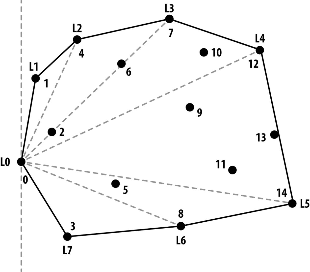
Figure 9-1. Sample set of points in plane with its convex hull drawn

Convex Hull Scan

Convex Hull Scan, invented by Andrew (1979), divides the problem by constructing a partial upper hull and a partial lower hull and then combining them. First, all points are sorted by their x coordinate (breaking ties by considering y). The partial upper hull starts with the leftmost two points in P. Convex Hull Scan extends the partial upper hull by finding the point p ∈ P whose x coordinate comes next in sorted order after the partial upper hull’s last point L_i. Computing the lower hull is similar; to produce the final results, join the partial results together by their end points.

If the three points L_i−1, L_i and the candidate point p form a right turn, Convex Hull Scan extends the partial hull to include p. This decision is equivalent to computing the determinant of the 3×3 matrix shown in Figure 9-2, which represents the cross product cp. If cp < 0, then the three points determine a right turn and Convex Hull Scan continues on. If cp = 0 (the three points are collinear) or if cp > 0 (the three points determine a left turn), then the middle point L_i must be removed from the partial hull to retain its convex property. Convex Hull Scan computes the convex upper hull by processing all points up to the rightmost point. The lower hull is similarly computed (this time by choosing points in decreasing x coordinate value), and the two partial hulls are joined together.

Figure 9-2. Computing determinant decides whether points form right turn

CONVEX HULL SCAN SUMMARY

Best, Average, Worst: O(n log n)

convexHull (P)

sort P ascending by x coordinate (break ties by sorting y)

if n < 3 then return P

upper = {p0, p1}

for i = 2 to n-1 do

append pi to upper

while last three in upper make left turn do

remove middle of last three in upper

lower = {pn-1, pn-2}

for i = n-3 downto 0 do

append pi to lower

while last three in lower make left turn do

remove middle of last three in lower

join upper andlower (remove duplicate end points)

return computed hull

Sorting points is the largest cost for this algorithm.

Propose these two points as being on the upper hull.

A left turn means the last three hull points form a nonconvex angle.

Middle point was wrong choice so remove.

Similar procedure computes lower hull.

Stitch these together to form the convex hull.

Figure 9-3 shows Convex Hull Scan in action as it computes the partial upper hull. Note that the overall approach makes numerous mistakes as it visits every point in P from left to right, yet it adjusts by dropping—sometimes repeatedly—the middle of the last three points while it correctly computes the upper partial hull.

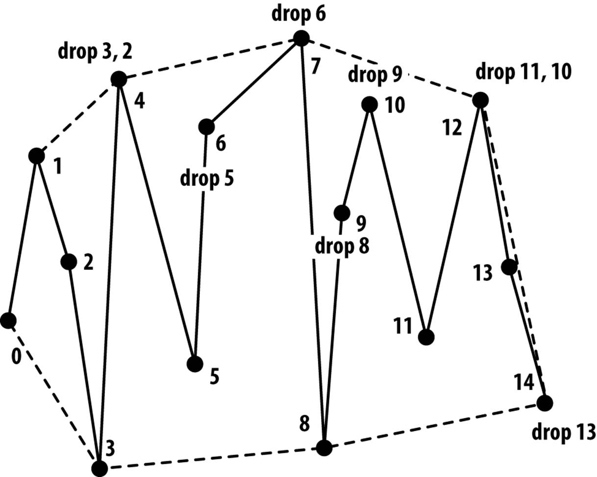
Figure 9-3. Incremental construction of upper partial convex hull

Input/Output

The input is a set of two-dimensional points P in a plane.

Convex Hull Scan computes an ordered list L containing the h vertices of the convex hull of P in clockwise order. The convex hull is a polygon defined by the points L₀, L₁,…, L_h−1, where h is the number of points in L. Note that the polygon is formed from the h line segments <L₀, L₁>,<L₁, L₂>,…, <L_h−1, L₀>.

To avoid trivial solutions, we assume |P| ≥ 3. No two points are “too close” to each other (as determined by the implementation). If two points are too close to each other and one of those points is on the convex hull, Convex Hull Scan might incorrectly select an invalid convex hull point (or discard a valid convex hull point); however, the difference would be negligible.

Context

Convex Hull Scan requires only primitive operations (such as multiply and divide), making it easier to implement than GrahamScan (Graham, 1972), which uses trigonometric identities as demonstrated in Chapter 3. Convex Hull Scan can support a large number of points because it is not recursive.

The fastest implementation occurs if the input set is uniformly distributed and thus can be sorted in O(n) using Bucket Sort, because the resulting performance would also be O(n). Without such information, we choose Heap Sort to achieve O(n log n) behavior for sorting the initial points. The supporting code repository contains each of the described implementations that we benchmark for performance.

Solution

Example 9-1 shows how Convex Hull Scan first computes the partial upper hull before reversing direction and computing the partial lower hull. The final convex hull is the combination of the two partial hulls.

Example 9-1. Convex Hull Scan solution to convex hull

public class ConvexHullScan implements IConvexHull {

public IPoint [] compute (IPoint[] points) {

// sort by x coordinate (and if ==, by y coordinate).

int n = points.length;

new HeapSort<IPoint>().sort (points, 0, n-1, IPoint.xy_sorter);

if (n < 3) { return points; }

// Compute upper hull by starting with leftmost two points

PartialHull upper = new PartialHull (points[0], points[1]);

for (int i = 2; i < n; i++) {

upper.add (points[i]);

while (upper.hasThree() && upper.areLastThreeNonRight()) {

upper.removeMiddleOfLastThree();

}

}

// Compute lower hull by starting with rightmost two points

PartialHull lower = new PartialHull (points[n-1], points[n-2]);

for (int i = n-3; i >= 0; i--) {

lower.add (points[i]);

while (lower.hasThree() && lower.areLastThreeNonRight()) {

lower.removeMiddleOfLastThree();

}

}

// remove duplicate end points when combining.

IPoint[] hull = new IPoint[upper.size()+lower.size()-2];

System.arraycopy (upper.getPoints(), 0, hull, 0, upper.size());

System.arraycopy (lower.getPoints(), 1, hull,

upper.size(), lower.size()-2);

return hull;

}

}

Because the first step of this algorithm must sort the points, we rely on Heap Sort to achieve the best average performance without suffering from the worst-case behavior of Quicksort. However, in the average case, Quicksort will outperform Heap Sort.

The Akl-Toussaint heuristic (1978) can noticeably improve the performance of the overall algorithm by discarding all points that exist within the extreme quadrilateral (the minimum and maximum points along both the x and y axes) computed from the initial set P. Figure 9-4 shows the extreme quadrilateral for the sample points from Figure 9-1. The discarded points are shown in gray; none of these points can belong to the convex hull.

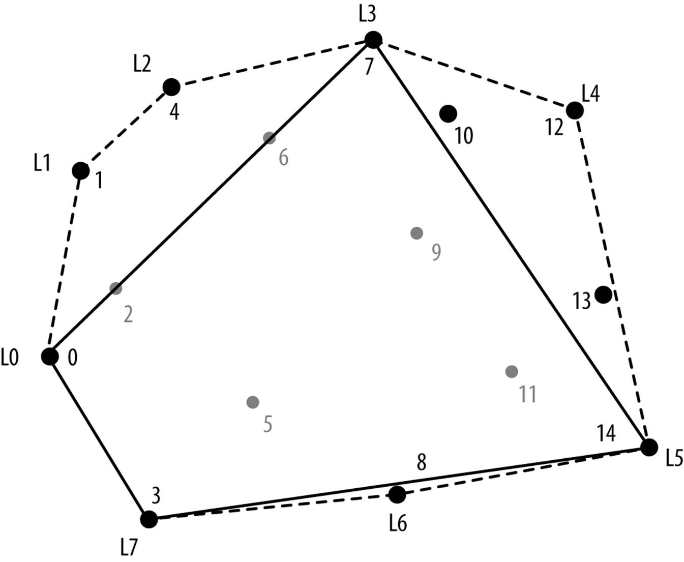
Figure 9-4. The Akl-Toussaint heuristic at work

To determine whether a point p is within the extreme quadrilateral, imagine a line segment s from p to an extreme point at (p.x, –∞), and count the number of times s intersects the four line segments of the quadrilateral; if the count is 1, p is inside and can be eliminated. The implementation handles special cases, such as when line segment s exactly intersects one of the end points of the extreme quadrilateral. This computation requires a fixed number of steps, so it is O(1), which means applying the Akl-Toussaint heuristic to all points is O(n). For large random samples, this heuristic can remove nearly half the initial points, and because these points are discarded before the sort operation, the costly sorting step in the algorithm is reduced.

Analysis

We ran a set of 100 trials on randomly generated two-dimensional points from the unit square, and the best and worst trials were discarded. Table 9-2 shows the average performance results of the remaining 98 trials. The table also shows the breakdown of average times to perform the heuristic plus some information about the solution that explains why Convex Hull Scan is so efficient.

As the size of the input set increases, nearly half of its points can be removed by the Akl-Toussaint heuristic. More surprising, perhaps, is the low number of points on the convex hull. The second column in Table 9-2 validates the claim by Preparata and Shamos (1985) that the number of points on the convex hull should be O(log n). Naturally, the distribution matters: if you choose points uniformly from a unit circle, for example, the convex hull contains on the order of the cube root of n points.

The first step in Convex Hull Scan explains the cost of O(n log n) when the points are sorted using one of the standard comparison-based sorting techniques described in Chapter 4. The for loop that computes the upper partial hull processes n − 2 points, the inner while loop cannot execute more than n − 2 times, and the same logic applies to the loop that computes the lower partial hull. The total time for the remaining steps of Convex Hull Scan is thus O(n).

Problems with floating-point arithmetic appear when Convex Hull Scan computes the cross-product calculation. Instead of strictly comparing whether the cross product cp < 0, PartialHull determines whether cp < δ, where δ is 10⁻⁹.

Variations

The sorting step of Convex Hull Scan can be eliminated if the points are already known to be in sorted order; in this case, Convex Hull Scan can perform in O(n). Alternatively, if the input points are drawn from a uniform distribution, then one can use Bucket Sort (see “Bucket Sort” inChapter 4) to also achieve O(n) performance. Another convex hull variation known as QuickHull (Eddy, 1977) uses the Divide and Conquer strategy inspired by Quicksort to compute the convex hull in O(n) performance on uniformly distributed points.

There is one final variation to consider. Convex Hull Scan doesn’t actually need a sorted array when it constructs the partial upper hull; it just needs to iterate over all points in P in order, from smallest x coordinate to highest x coordinate. This behavior is exactly what occurs if one constructs a binary heap from the points in P and repeatedly removes the smallest element from the heap. If the removed points are stored in a linked list, the points can be simply “read off” the linked list to process the points in reverse order from right to left. The code for this variation (identified as Heap in Figure 9-5) is available in the code repository accompanying this book.

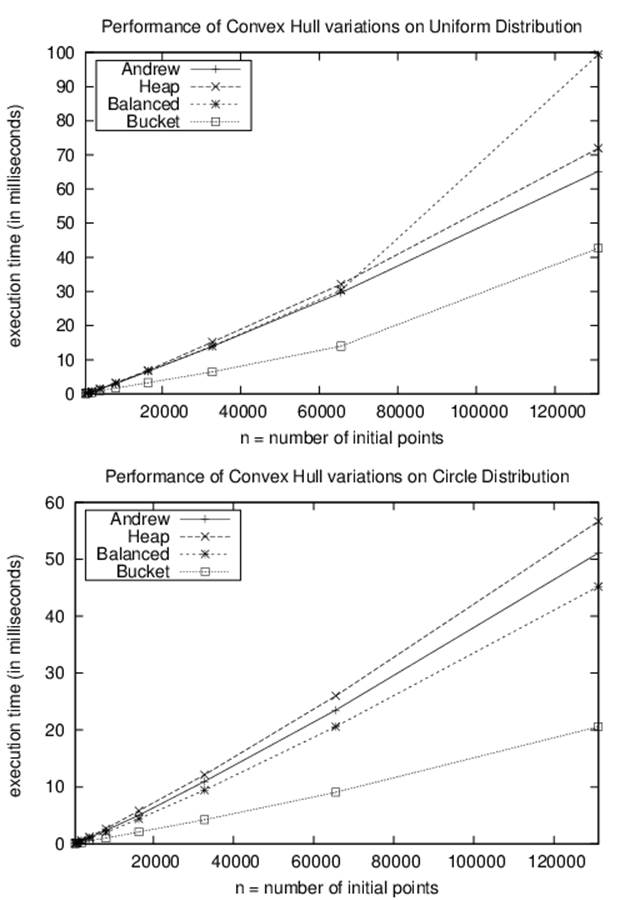
Figure 9-5. Performance of convex hull variations

The performance results shown in Figure 9-5 were generated from two data set distributions:

Circle data

n points distributed evenly over the edge of a unit circle. All points will belong to the convex hull, so this is an extreme case.

Uniform data

n points distributed evenly from the unit square. As n increases, the majority of these points will not be part of the convex hull, so this represents another extreme case.

We ran a series of trials using data sets with 512 to 131,072 points, the two data set distributions, the different implementations described in Example 9-1, and the code repository. We did not employ the Akl-Toussaint heuristic. For each data set size, we ran 100 trials and discarded the best- and worst-performing runs. The resulting average time (in milliseconds) of the remaining 98 trials is depicted in Figure 9-5. The implementation using balanced binary trees shows the best performance of the approaches that use comparison-based sorting techniques. Note that the implementation using Bucket Sort offers the most efficient implementation, but only because the input set is drawn from a uniform distribution. In the general case, computing a convex hull can be performed in O(n log n).

However, these implementations also suffer poor performance should the input data be skewed. Consider n points distributed unevenly with with points (0,0), (1,1) and n − 2 points clustered in thin slices just to the left of .502. This data set is constructed to defeat Bucket Sort. Table 9-3shows how Bucket Sort degenerates into an O(n²) algorithm because it relies on Insertion Sort to sort its buckets.

The convex hull problem can be extended to three dimensions and higher where the goal is to compute the bounding polyhedron surrounding the three-dimensional point space. Unfortunately, in higher dimensions, more complex implementations are required.

Melkman (1987) developed an algorithm that produces the convex hull for a simple polyline or polygon in O(n). Quite simply, it avoids the need to sort the initial points by taking advantage of the ordered arrangement of points in the polygon itself.

A convex hull can be maintained efficiently using an approach proposed by Overmars and van Leeuwen (1981). The convex hull points are stored in a tree structure that supports both deletion and insertion of points. The cost of either an insert or delete is known to be O(log² n), so the overall cost of constructing the hull becomes O(n log² n) while still requiring only O(n) space. This result reinforces the principle that every performance benefit comes with its own trade-off.

GrahamScan was one of the earliest convex hull algorithms, developed in 1972 using simple trigonometric identities. We described this algorithm in Chapter 3. Using the determinant computation shown earlier, an appropriate implementation needs only simple data structures and basic mathematical operations. GrahamScan computes the convex hull in O(n log n), because it first sorts points by the angles they make with the point s ∈ P with the smallest y coordinate and the x axis. One challenge in completing this sort is that points with the same angle must be ordered by their distance from s.

Computing Line-Segment Intersections

Given a set of n line segments S in a two-dimensional plane, you might need to determine the full set of intersection points between all segments. In the example in Figure 9-6, there are two intersections (shown as small black circles) found in this set of four line segments. As shown inExample 9-2, a brute-force approach will compute all C(n,2) or n*(n – 1)/2 intersections of the line segments in S using O(n²) time. For each pair, the implementation outputs the intersection, if it exists.

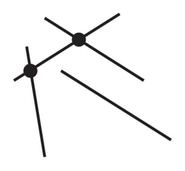
Figure 9-6. Three line segments with two intersections

Example 9-2. Brute Force Intersection implementation

public class BruteForceAlgorithm extends IntersectionDetection {

public Hashtable<IPoint, List<ILineSegment>> intersections

(ILineSegment[] segments) {

initialize();

for (int i = 0; i < segments.length-1; i++) {

for (int j = i+1; j < segments.length; j++) {

IPoint p = segments[i].intersection (segments[j]);

if (p != null) {

record (p, segments[i], segments[j]);

}

}

}

return report;

}

}

This computation requires O(n²) individual intersection computations and may require complex trigonometric functions.

It is not immediately clear that any improvement over O(n²) is possible, yet this chapter presents the innovative LineSweep algorithm, which on average shows how to compute the results in O((n + k) log n) where k represents the number of reported intersection points.

LineSweep

There are numerous situations where we must detect intersections between geometric shapes. In VLSI chip design, precise circuits are laid out on a circuit board, and there must be no unplanned intersections. For travel planning, a set of roads could be stored in a database as line segments whose street intersections are determined by line-segment intersections.

Figure 9-7 shows an example with seven intersections between six line segments. Perhaps we don’t have to compare all possible C(n, 2) or n*(n – 1)/2 line-segment pairs. After all, line segments that are clearly apart from one another (in this example, S1 and S4) cannot intersect. LineSweepis a proven approach that improves efficiency by focusing on a subset of the input elements as it progresses. Imagine sweeping a horizontal line L across the input set of line segments from the top to the bottom and reporting the intersections when they are found by L. Figure 9-7 shows the state of line L as the sweep occurs from top to bottom (at nine distinct and specific locations).

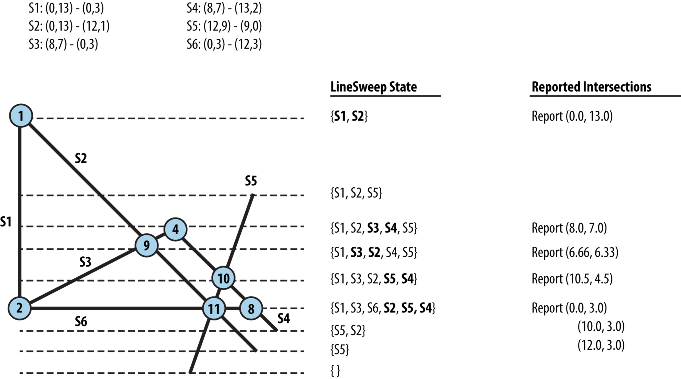
Figure 9-7. Detecting seven intersections for six line segments

The innovation of LineSweep is in recognizing that line segments can be ordered from left to right at a specific y coordinate. Horizontal segments are addressed by considering the left end point to be “higher” than the right end point. Line-segment intersections can then occur only between neighboring segments in the state of the sweep line. Specifically, for two line segments s_i and s_j to intersect, there must be some time during the line sweep when they are neighbors. LineSweep can efficiently locate intersections by maintaining this line state.

Looking closer at the nine selected locations of the horizontal sweep line in Figure 9-7, you will see that each occurs at (i) the start or end of a line segment, or (ii) an intersection. LineSweep doesn’t actually “sweep” a line across the Cartesian plane; rather, it inserts the 2*n segment end points into an event queue, which is a modified priority queue. All intersections involving start and end points of existing line segments can be detected when processing these points. LineSweep processes the queue to build up the state of the sweep line L to determine when neighboring line segments intersect.

Input/Output

LineSweep processes a set of n line segments S in the Cartesian plane. There can be no duplicate segments in S. No two line segments in S are collinear (i.e., overlap each other and have the same slope). The algorithm supports both horizontal and vertical line segments by carefully performing computations and ordering segments appropriately. No line segment should be a single point (i.e., a line segment whose start and end point are the same).

The output contains the k points representing the intersections (if any exist) between these line segments and, for each of these k points, p_i, the actual line segments from S that intersect at p_i.

Context

When the expected number of intersections is much smaller than the number of line segments, this algorithm handily outperforms a brute-force approach. When there are a significant number of intersections, the bookkeeping of the algorithm may outweigh its benefits.

A sweep-based approach is useful when you can (a) efficiently construct the line state, and (b) manage the event queue that defines when the sweep line is interpreted. There are numerous special cases to consider within the LineSweep implementation, and the resulting code is much more complex than the brute-force approach, whose worst-case performance is O(n²). Choose this algorithm because of the expected performance savings and improved worst-case behavior.

LineSweep produces partial results incrementally until the entire input set has been processed and all output results are produced. In the example here, the line state is a balanced binary tree of line segments, which is possible because we can impose an ordering on the segments at the sweep line. The event queue can also simply be a balanced binary tree of event points sorted lexicographically, meaning that points with a higher y value appear first (because the sweep line moves down the Cartesian plane from top to bottom); if there are two points with the same y value, the one with the lower x value appears first.

To simplify the coding of the algorithm, the binary tree used to store the line state is an augmented balanced binary tree in which only the leaf nodes contain actual information. The interior nodes store min and max information about the leftmost segment in the left subtree and rightmost segment in the right subtree. The ordering of segments within the tree is made based on the sweep point, the current EventPoint being processed from the priority queue.

LINESWEEP SUMMARY

Best, Average, Worst: O((n + k) log n)

intersection (S)

EQ = new EventQueue

foreach s in S do

ep = find s.start in EQ orcreate new one andinsert into EQ

add s to ep.upperLineSegments

ep = find s.end in EQ orcreate new one andinsert into EQ

add s to ep.lowerLineSegments

state = new lineState

while EQ is notempty do

handleEvent (EQ, state, getMin(EQ))

end

handleEvent (EQ, state, ep)

left = segment in state to left of ep

right = segment in state to right of ep

compute intersections in state between left to right

remove segments in state between left andright

advance state sweep point down to ep

if new segments start at ep then

insert new segments into state

update = true

if intersections associated with ep then

insert intersections into state

update = true

if update then

updateQueue (EQ, left, left successor)

updateQueue (EQ, right, right predecessor)

else

updateQueue (EQ, left, right)

end

updateQueue (EQ, A, B)

if neighboring A andB segments intersect below sweep point then

insert their intersection point into EQ

end

Initialize event queue with up to 2*n points.

Event points refer to segments (upper or lower end points).

Any intersection occurs between neighboring line segments.

Maintain line state as new segments are discovered below sweep line.

At an intersection, neighboring line segments switch relative position.

Add intersection to event queue only if below sweep line.

Solution

The solution described in Example 9-3 depends on the EventPoint, EventQueue, and LineState classes found in the code repository.

Example 9-3. LineSweep Java implementation

public class LineSweep extends IntersectionDetection {

// Store line sweep state and event queue

LineState lineState = new LineState();

EventQueue eq = new EventQueue();

/** Compute intersection of all segments from array of segments. */

public Hashtable<IPoint,ILineSegment[]> intersections (

ILineSegment[] segs) {

// Construct Event Queue from segments. Ensure only unique

// points appear by combining all information as it is discovered.

for (ILineSegment ils : segs) {

EventPoint ep = new EventPoint (ils.getStart());

EventPoint existing = eq.event (ep);

if (existing == null) { eq.insert (ep); } else { ep = existing; }

// add upper line segments to ep (the object in the queue)

ep.addUpperLineSegment (ils);

ep = new EventPoint (ils.getEnd());

existing = eq.event (ep);

if (existing == null) { eq.insert (ep); } else { ep = existing; }

// add lower line segments to ep (the object in the queue)

ep.addLowerLineSegment (ils);

}

// Sweep top to bottom, processing each Event Point in the queue.

while (!eq.isEmpty()) {

EventPoint p = eq.min();

handleEventPoint (p);

}

// return report of all computed intersections

return report;

}

// Process events by updating line state and reporting intersections.

private void handleEventPoint (EventPoint ep) {

// Find segments, if they exist, to left (and right) of ep in

// linestate. Intersections can happen only between neighboring

// segments. Start with nearest ones because as line sweeps down

// we will find any other intersections that (for now) we put off.

AugmentedNode<ILineSegment> left = lineState.leftNeighbor (ep);

AugmentedNode<ILineSegment> right = lineState.rightNeighbor (ep);

// determine intersections 'ints' from neighboring line segments and

// get upper segments 'ups' and lower segments 'lows' for this event

// point. An intersection exists if > 1 segment is associated with

// event point.

lineState.determineIntersecting (ep, left, right);

List<ILineSegment> ints = ep.intersectingSegments();

List<ILineSegment> ups = ep.upperEndpointSegments();

List<ILineSegment> lows = ep.lowerEndpointSegments();

if (lows.size() + ups.size() + ints.size() > 1) {

record (ep.point, new List[] { lows, ups, ints } );

}

// Delete everything after left until left's successor is right.

// Then update the sweep point, so insertions will be ordered. Only

// ups and ints are inserted because they are still active.

lineState.deleteRange (left, right);

lineState.setSweepPoint (ep.point);

boolean update = false;

if (!ups.isEmpty()) {

lineState.insertSegments (ups);

update = true;

}

if (!ints.isEmpty()) {

lineState.insertSegments (ints);

update = true;

}

// If state shows no intersections at this event point, see if left

// and right segments intersect below sweep line, and update event

// queue properly. Otherwise, if there was an intersection, the order

// of segments between left & right have switched so we check two

// specific ranges, namely, left and its (new) successor, and right

// and its (new) predecessor.

if (!update) {

if (left != null && right != null) { updateQueue (left, right); }

} else {

if (left != null) { updateQueue (left, lineState.successor (left)); }

if (right != null) { updateQueue (lineState.pred (right), right); }

}

}

// Any intersections below sweep line are inserted as event points.

private void updateQueue (AugmentedNode<ILineSegment> left,

AugmentedNode<ILineSegment> right) {

// If two neighboring line segments intersect. make sure that new

// intersection point is *below* the sweep line and not added twice.

IPoint p = left.key().intersection (right.key());

if (p == null) { return; }

if (EventPoint.pointSorter.compare (p,lineState.sweepPt) > 0) {

EventPoint new_ep = new EventPoint (p);

if (!eq.contains (new_ep)) { eq.insert (new_ep); }

}

}

}

When the EventQueue is initialized with up to 2*n EventPoint objects, each stores the ILineSegment objects that start (known as upper segments) and end (known as lower segments) at the stored IPoint object. When LineSweep discovers an intersection between line segments, anEventPoint representing that intersection is inserted into the EventQueue as long as it occurs below the sweep line. In this way, no intersections are missed and none are duplicated. For proper functioning, if this intersecting event point already exists within the EventQueue, the intersecting information is updated within the queue rather than being inserted twice. It is for this reason that LineSweep must be able to determine whether the event queue contains a specific EventPoint object.

In Figure 9-7, when the event point representing the lower point for segment S6 (technically the rightmost end point, because S6 is horizontal) is inserted into the priority queue, LineSweep only stores S6 as a lower segment; once it is processed, it will additionally store S4 as an intersecting segment. For a more complex case, when the event point representing the intersection of segments S2 and S5 is inserted into the priority queue, it stores no additional information. But after this event point is processed, it will store segments S6, S2, and S5 as intersecting segments.

The computational engine of LineSweep is the LineState class, which maintains the current sweep point as it sweeps from the top of the Cartesian plane downward. When the minimum entry is extracted from the EventQueue, the provided pointSorter comparator properly returns theEventPoint objects from top to bottom and left to right.

The true work of LineSweep occurs in the determineIntersecting method of LineState: the intersections are determined by iterating over those segments between left and right. Full details on these supporting classes are found in the code repository.

LineSweep achieves O((n + k) log n) performance because it can reorder the active line segments when the sweep point is advanced. If this step requires more than O(log s) for its operations, where s is the number of segments in the state, the performance of the overall algorithm will degenerate to O(n²). For example, if the line state was stored simply as a doubly linked list (a useful structure to rapidly find predecessor and successor segments), the insert operation would increase to require O(s) time to properly locate the segment in the list, and as the set s of line segments increases, the performance degradation would soon become noticeable.

Similarly, the event queue must support an efficient operation to determine whether an event point is already present in the queue. Using a heap-based priority queue implementation—as provided by java.util.PriorityQueue, for example—also forces the algorithm to degenerate to O(n²). Beware of code that claims to implement an O(n log n) algorithm but instead produces an O(n²) implementation!

Analysis

LineSweep inserts up to 2*n segment end points into an event queue, a modified priority queue that supports the following operations in time O(log q), where q is the number of elements in the queue:

min

Remove the minimum element from the queue.

insert (e)

Insert e into its proper location within the ordered queue.

member (e)

Determine whether e is a member of the queue. This operation is not strictly required of a generic priority queue.

Only unique points appear in the event queue—in other words, if the same event point is re-inserted, its information is combined with the event point already in the queue. Thus, when the points from Figure 9-7 are initially inserted, the event queue contains only eight event points.

LineSweep sweeps from top to bottom and updates the line state by adding and deleting segments in their proper order. In Figure 9-7, the ordered line state reflects the line segments that intersect the sweep line, from left to right, after processing the event point. To properly compute intersections, LineSweep determines the segment in the state to the left of (or right of) a given segment s_i. LineSweep uses an augmented balanced binary tree to process all of the following operations in time O(log t), where t is the number of elements in the tree:

insert (s)

Insert line segment s into the tree.

delete (s)

Delete segment s from the tree.

previous (s)

Return segment immediately before s in the ordering, if one exists.

successor (s)

Return segment immediately after s in the ordering, if one exists.

To properly maintain the ordering of segments, LineSweep swaps the order of segments when a sweep detects an intersection between segments s_i and s_j; fortunately, this too can be performed in O(log t) time simply by updating the sweep line point and then deleting and reinserting the line segments s_i and s_j. In Figure 9-7, for example, this swap occurs when the third intersection (6.66, 6.33) is found.

The initialization phase of the algorithm constructs a priority queue from the 2*n points (start and end) in the input set of n lines. The event queue must additionally be able to determine whether a new point p already exists within the queue; for this reason, we cannot simply use a heap to store the event queue, as is commonly done with priority queues. Since the queue is ordered, we must define an ordering of two-dimensional points. Point p₁ < p₂ if p₁.y > p₂.y; however, if p₁.y = p₂.y, then p₁ < p₂ if p₁.x < p₂.x. The size of the queue will never be larger than 2*n + k, where kis the number of intersections and n is the number of input line segments.

All intersection points detected by LineSweep below the sweep line are added to the event queue, where they will be processed to swap the order of intersecting segments when the sweep line finally reaches the intersection point. Note that all intersections between neighboring segments will be found below the sweep line, and no intersection point will be missed.

As LineSweep processes each event point, line segments are added to the state when an upper end point is visited, and removed when a lower end point is visited. Thus, the line state will never store more than n line segments. The operations that probe the line state can be performed in O(log n) time, and because there are never more than O(n + k) operations over the state, our cost is O((n + k) log (n + k)). Because k is no larger than C(n, 2) or n*(n – 1)/2, performance is O((n + k) log n), which becomes O(n² log n) in the worst case.

The performance of LineSweep is dependent on complex properties of the input (i.e., the total number of intersections and the average number of line segments maintained by the sweep line at any given moment). We can benchmark its performance given a specific problem and input data. We’ll discuss two such problems now.

An interesting problem from mathematics is how to compute an approximate value of π using just a set of toothpicks and a piece of paper (known as Buffon’s needle problem). If the toothpicks all are len units long, draw a set of vertical lines on the paper d units apart from one another whered ≥ len. Randomly toss n toothpicks on the paper and let k be the number of intersections with the vertical lines. It turns out that the probability that a toothpick intersects a line (which can be computed as k/n) is equal to (2*len)/(π*d).

When the number of intersections is much less than n², the brute-force approach wastes time checking lines that don’t intersect (as shown in Table 9-4). When there are many intersections, the determining factor will be the average number of line segments maintained by LineState during the duration of LineSweep. When it is low (as might be expected with random line segments in the plane), LineSweep will be the winner.

For the second problem, consider a set S where there are O(n²) intersections among the line segments. LineSweep will seriously underperform because of the overhead in maintaining the line state in the face of so many intersections. Table 9-5 shows how brute force handily outperformsLineSweep, where n is the number of line segments whose intersection creates the C(n, 2) or n*(n – 1)/2 intersection points.

Variations

One interesting variation requires only that the algorithm report one of the intersection points, rather than all points; this would be useful to detect whether two polygons intersect. This algorithm requires only O(n log n) time, and may more rapidly locate the first intersection in the average case. Another variation considers an input set of red and blue lines where the only desired intersections are those between different colored line segments (Palazzi and Snoeyink, 1994).

Voronoi Diagram

In 1986, Fortune applied the line-sweep technique to solve another computational geometry problem, namely, constructing the Voronoi diagram for a set of points, P, in the Cartesian plane. This diagram is useful in a number of disciplines, ranging from the life sciences to economics (Aurenhammer, 1991).

A Voronoi diagram partitions a plane into regions based on each region’s distance to a set of n two-dimensional points, P. Each of the n regions consists of the Cartesian points closer to point p_i ∈ P than any other p_j ∈ P. Figure 9-8 shows the computed Voronoi diagram (black lines) for 13 sample points (shown as squares). The Voronoi diagram consists of 13 convex regions formed from edges (the lines in the figure) and vertices (where these lines intersect). Given the Voronoi diagram for a set of points, you can:

§ Compute the convex hull

§ Determine the largest empty circle within the points

§ Find the nearest neighbor for each point

§ Find the two closest points in the set

Fortune Sweep implements a line sweep similar to the one used to detect where line segments intersect. Recall that a line sweep inserts existing points into a priority queue and processes those points in order, thus defining a sweep line. The algorithm maintains a line state that can be updated efficiently to determine the Voronoi diagram. In Fortune Sweep, the key observation to make is that the sweeping line divides the plane into three distinct regions, as shown in Figure 9-9.

As the line sweeps down the plane, a partial Voronoi diagram is formed; in Figure 9-9, the region associated with point p₂ is fully computed as a semi-infinite polygon delimited by four line segments, shown in bold. The sweep line is currently ready to process point p₆ and points p₇ throughp₁₁ are waiting to be processed. The line-state structure currently maintains points { p₁, p₄, p₅, and p₃ }.

The challenge in understanding Fortune Sweep is that the line state is a complex structure called a beach line. In Figure 9-9, the beach line is the thin collection of curved fragments from left to right; the point where two parabolas meet is known as a breakpoint, and the dashed lines represent partial edges in the Voronoi diagram that have yet to be confirmed. Each of the points in the beach line state defines a parabola with respect to the sweep line. The beach line is defined as the intersection of these parabolas closest to the sweep line.

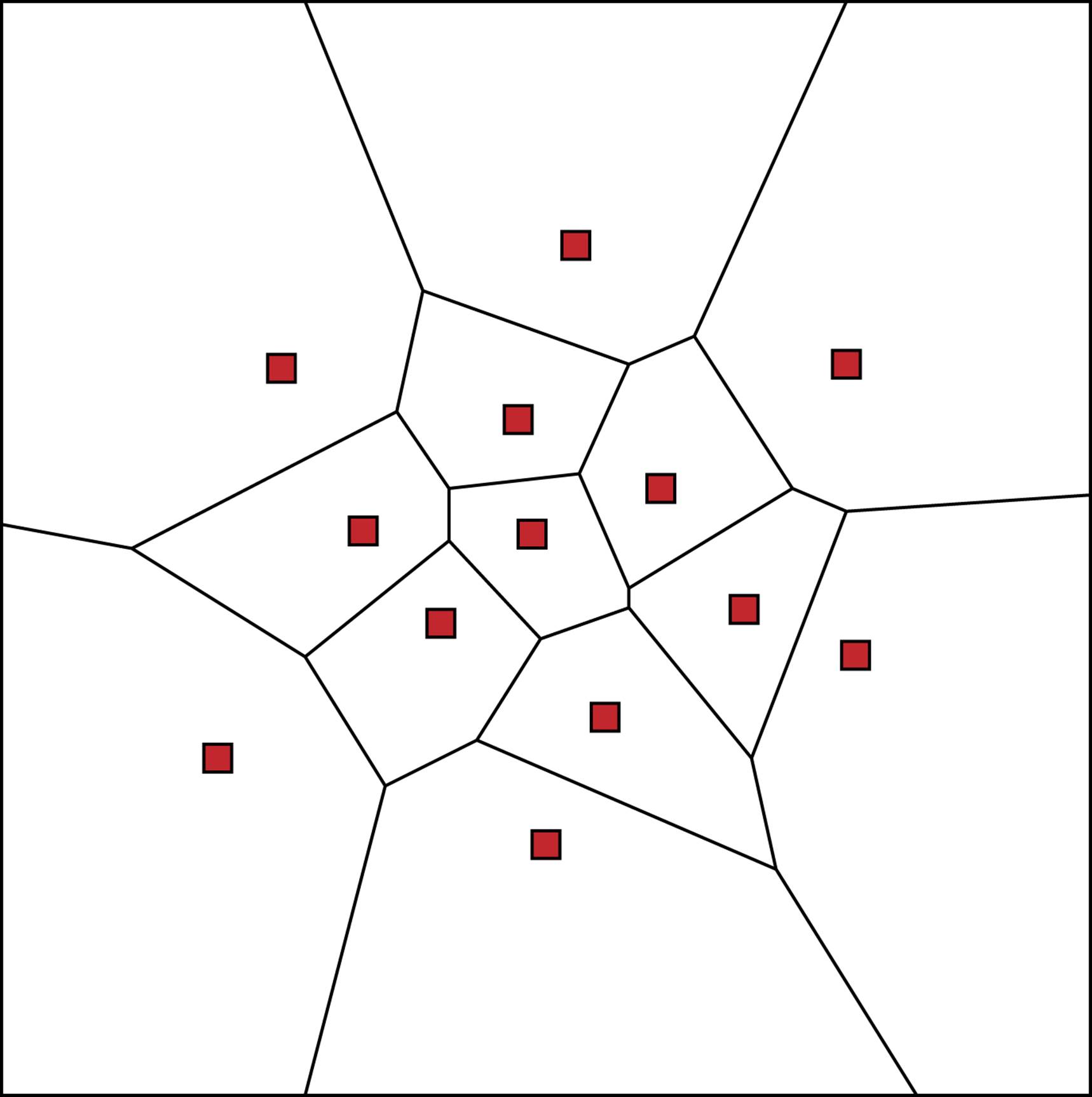
Figure 9-8. Sample Voronoi diagram

To explain the structure of the curved segments in the beach line, we need to define the parabola geometric shape. Given a focus point, f, and a line, L, a parabola is a symmetric shape composed of the Cartesian points that are equidistant from f and the line L. The vertex of the parabola, v = (h, k), is the lowest point on the shape. p represents the distance between L and v as well as the distance between v and f. Given those variables, the equation 4p(y – k) = (x – h)² defines the parabola’s structure, which is easy to visualize when L is a horizontal line and the parabola opens upward as shown in Figure 9-10.

The sweep starts at the topmost point in P and sweeps downward, discovering points known as sites to process. The parabolas in the beach line change shape as the sweep line moves down, as shown in Figure 9-11, which means that breakpoints also change their location. Fortunately, the algorithm updates the sweep line only O(n) times.

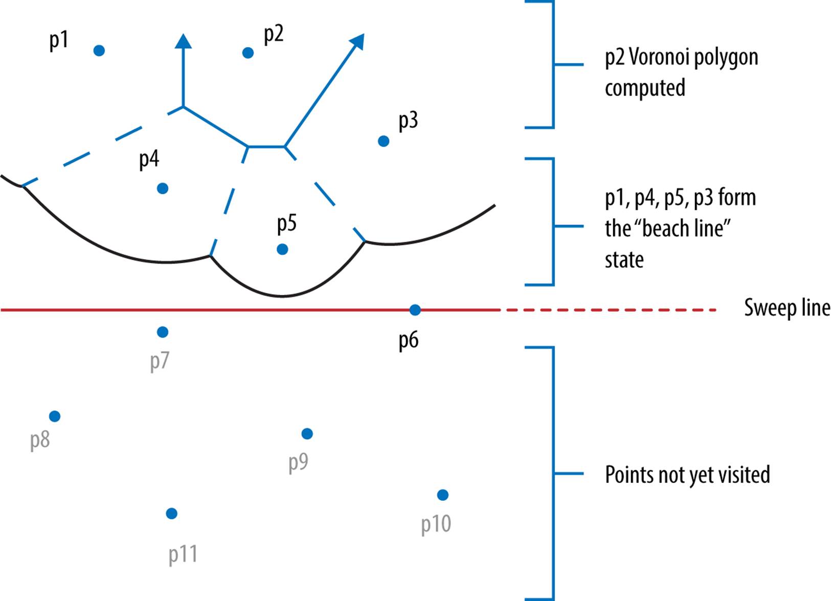
Figure 9-9. Elements of Fortune Sweep

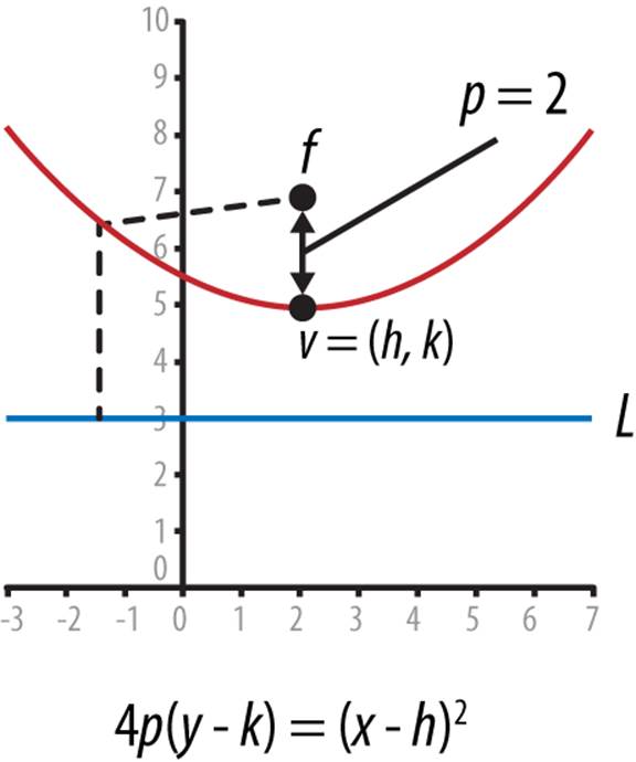
Figure 9-10. Definition of parabola

A vertex in the Voronoi diagram is computed by detecting three points in P that lie on a circle that doesn’t contain any other points in P. The center of this circle defines the Voronoi vertex, because that is a point equidistant from the three points. The three rays that radiate from the center become edges in the Voronoi diagram because these lines define the points that are equidistant from two points in the collection. These edges bisect the chord line segments in the circle between the points. For example, line L₃ in Figure 9-12 is perpendicular to the line segment that would be drawn between (r₁, r₃).

Figure 9-11. Parabolas change shape as the sweep line moves down

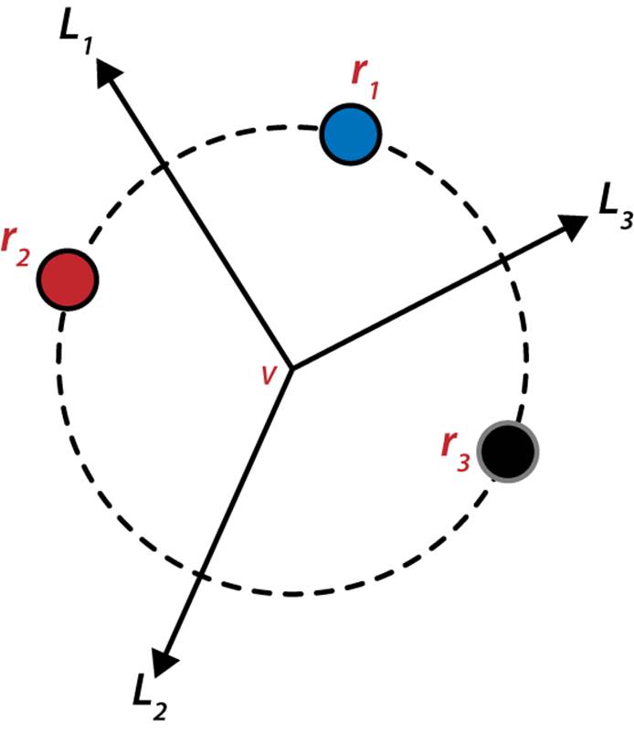
Figure 9-12. Circle formed by three points

We now show how Fortune Sweep maintains state information to detect these circles. The characteristics of the beach line minimize the number of circles Fortune Sweep checks; specifically, whenever the beach line is updated, Fortune Sweep needs to check only the neighboring arcs (to the left and to the right) where the update occurred. Figure 9-12 shows the mechanics of Fortune Sweep with just three points. These three points are processed in order from top to bottom, namely, r₁, r₂, and r₃. A circle is defined once the third point is processed and is known as thecircumcircle of these three points.

Figure 9-13 shows the state of the beach line after processing points r₁ and r₂. The beach line is formed by the parabola segments that are closest to the sweep line; in this case, the state of the sweep line is represented as a binary tree where leaf nodes declare the associated parabola segment and internal nodes represent breakpoints. The beach line, from left to right, is formed by three parabolic segments, s₁, s₂ and then s₁ again, which are drawn from the parabolas associated with points r₁, r₂ and then r₁ again. The breakpoint s₁:s₂ represents the x coordinate where to its left, parabola s₁ is closer to the sweep line, and to its right, parabola s₂ is closer to the sweep line. The same characteristics holds for breakpoint s₂:s₁.

Figure 9-13. Beach line after two points

Figure 9-14 shows when the line-sweep processes the third point, r₃. By its location, a vertical line through r₃ intersects the beach line at the rightmost arc, s₁, and the updated beach line state is shown on the right side in Figure 9-14. There are four nonleaf nodes, representing the four intersections that occur on the beach line between the three parabolas. There are five leaf nodes, representing the five arc segments that form the beach line, from left to right.

Once this beach line is formed, observe that these three points form a circumcircle. The center of the circle has the potential to become a Voronoi point in the diagram, but this will happen only if no other point in P is contained within the circle. The algorithm handles this situation elegantly by creating a circle event, whose coordinates are the lowest point on this circle (shown in Figure 9-15), and inserting that event into the event priority queue. Should some other site event be processed before this circle event that “gets in the way,” this circle event will be eliminated. Otherwise, it will be processed in turn and the center point of the circle becomes a vertex in the Voronoi diagram.

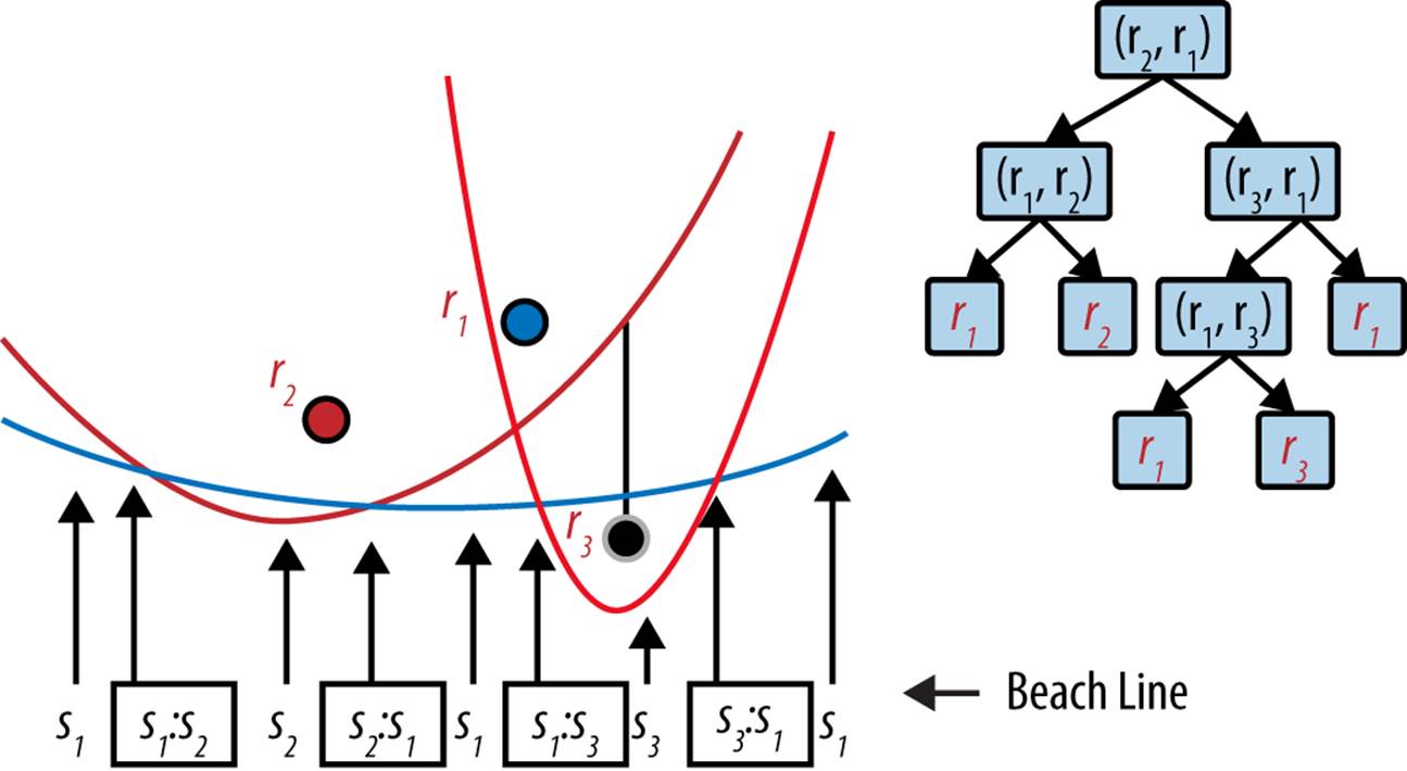
Figure 9-14. Beach line after three points

A key step in this algorithm is the removal of nodes from the beach line state that can have no other effect on the construction of the Voronoi diagram. Once the identified circle event is processed, the middle arc, associated with r₁ in this case, has no further effect on any other point in P, so it can be removed from the beach line. The resulting beach line state is shown in the binary tree on the right side of Figure 9-15.

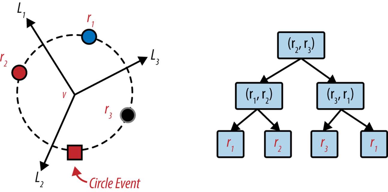
Figure 9-15. Beach line after processing circle event

Input/Output

The input is a set of two-dimensional points P in a plane.

Fortune Sweep computes a Voronoi diagram composed of n Voronoi polygons, each of which defines the region for one of the points in P. Mathematically, there may be partially infinite regions, but the algorithm eliminates these by computing the Voronoi diagram within a bounding box of suitable size to enclose all points in P. The output will be a set of line segments and Voronoi polygons that are defined by edges in clockwise order around each point in P.

Some implementations assume P does not contain four cocircular points that form a circle.

Some implementations assume that no two points share the same x or y coordinate. Doing so eliminates many of the special cases. This is easy to implement when the input set (x, y) contains integer coordinates: simply add a random fractional number to each coordinate before invokingFortune Sweep.

Solution

The implementation is complicated because of the computations needed to maintain the beach line’s state; some of the special cases are omitted from the presentation here. The code repository contains functions that perform the geometric computations of intersecting parabolas. The classes that support this implementation are summarized in Figure 9-16. This implementation uses Python’s heapq module, which provides heappop and heappush methods used to construct and process a priority queue.

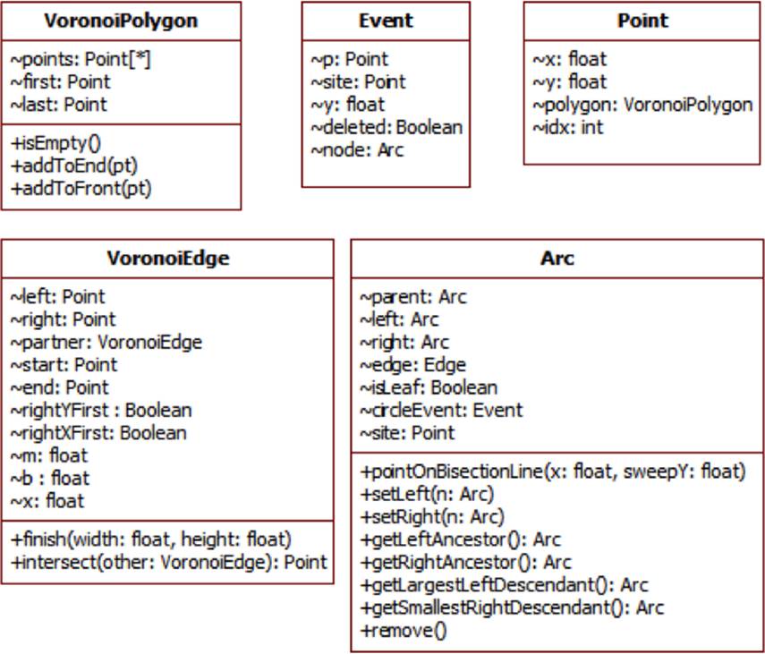
Figure 9-16. Classes supporting the code

As shown in Example 9-4, the process method creates site events for each of the input points and processes each event one at a time by descending y coordinate (ties are broken by smaller x coordinate).

FORTUNE SWEEP SUMMARY

Best, Average, Worst: O(n log n)

fortune (P)

PQ = new Priority Queue

LineState = new Binary Tree

foreach p in P do

event = new SiteEvent(p)

insert event into PQ

while PQ is notempty do

event = getMin(PQ)

sweepPt = event.p

if event is site event then

processSite(event)

else

processCircle(event)

finishEdges()

processSite(e)

leaf = find arc A in beach line bisected by e.p

modify beach line andremove unneeded circle events

detect new potential circle events

processCircle(e)

determine (left,right) neighboring arcs in beach line

remove unneeded circle events

record Voronoi vertex andVoroni edges

modify beach line to remove "middle" arc

detect new potential circle events to left andright

Priority queue orders events by descending y coordinate.

Sweep line is updated by point associated with each event removed.

Remaining breakpoints in beach line determine final edges.

Update beach line with each new point…

…which might remove potential circle events.

Compute Voronoi point and update beach line state.

Example 9-4. Voronoi Python implementation

from heapq import heappop, heappush

class Voronoi:

def process (self, points):

self.pq = []

self.edges = []

self.tree = None

self.firstPoint = None # handle tie breakers with first point

self.stillOnFirstRow = True

self.points = []

# Each point has unique identifier

for idx inrange(len(points)):

pt = Point (points[idx], idx)

self.points.append (pt)

event = Event (pt, site=pt)

heappush (self.pq, event)

while self.pq:

event = heappop (self.pq)

if event.deleted:

continue

self.sweepPt = event.p

if event.site:

self.processSite (event)

else:

self.processCircle (event)

# complete edges that remain and stretch to infinity

if self.tree and notself.tree.isLeaf:

self.finishEdges (self.tree)

# Complete Voronoi Edges with partners

for e inself.edges:

if e.partner:

if e.b isNone:

e.start.y = self.height

else:

e.start = e.partner.end

The implementation handles the special case when there are multiple points that share the same largest y coordinate value; it does so by storing the firstPoint detected within processSite.

The true details of Fortune Sweep are contained within the processSite implementation shown in Example 9-5 and processCircle shown in Example 9-6.

Example 9-5. Voronoi process site event

def processSite (self, event):

if self.tree == None:

self.tree = Arc(event.p)

self.firstPoint = event.p

return

# Must handle special case when two points are at topmost y coordinate, in

# which case the root is a leaf node. Note that when sorting events, ties

# are broken by x coordinate, so the next point must be to the right.

if self.tree.isLeaf andevent.y == self.tree.site.y:

left = self.tree

right = Arc(event.p)

start = Point(((self.firstPoint.x + event.p.x)/2, self.height))

edge = VoronoiEdge (start, self.firstPoint, event.p)

self.tree = Arc(edge = edge)

self.tree.setLeft (left)

self.tree.setRight (right)

self.edges.append (edge)

return

# If leaf had a circle event, it is no longer valid

# since it is being split

leaf = self.findArc (event.p.x)

if leaf.circleEvent:

leaf.circleEvent.deleted = True

# find point on parabola where event.pt.x bisects with vertical line,

start = leaf.pointOnBisectionLine (event.p.x, self.sweepPt.y)

# Potential Voronoi edges discovered between two sites

negRay = VoronoiEdge (start, leaf.site, event.p)

posRay = VoronoiEdge (start, event.p, leaf.site)

negRay.partner = posRay

self.edges.append (negRay)

# modify beach line with new interior nodes

leaf.edge = posRay

leaf.isLeaf = False

left = Arc()

left.edge = negRay

left.setLeft (Arc(leaf.site))

left.setRight (Arc(event.p))

leaf.setLeft (left)

leaf.setRight (Arc(leaf.site))

# Check whether there is potential circle event on left or right.

self.generateCircleEvent (left.left)

self.generateCircleEvent (leaf.right)

The processSite method modifies the beach line with each discovered site event to insert two additional interior nodes and two additional leaf nodes. The findArc method, in O(log n) time, locates the arc that must be modified by the newly discovered site event. In modifying the beach line, the algorithm computes two edges that will ultimately be in the final Voronoi diagram. These are attached with the breakpoint Arc nodes in the tree. Whenever the beach line state changes, the algorithm checks to the left and to the right to determine whether neighboring arcs form a potential circle event.

Example 9-6. Voronoi process circle event

def processCircle (self, event):

node = event.node

# Find neighbor on the left and right.

leftA = node.getLeftAncestor()

left = leftA.getLargestDescendant()

rightA = node.getRightAncestor()

right = rightA.getSmallestDescendant()

# Eliminate old circle events if they exist.

if left.circleEvent:

left.circleEvent.deleted = True

if right.circleEvent:

right.circleEvent.deleted = True

# Circle defined by left - node - right. Terminate Voronoi rays.

p = node.pointOnBisectionLine (event.p.x, self.sweepPt.y)

leftA.edge.end = p

rightA.edge.end = p

# Update ancestor node in beach line to record new potential edges.

t = node

ancestor = None

while t != self.tree:

t = t.parent

if t == leftA:

ancestor = leftA

elif t == rightA:

ancestor = rightA

ancestor.edge = VoronoiEdge(p, left.site, right.site)

self.edges.append (ancestor.edge)

# Remove middle arc (leaf node) from beach line tree.

node.remove()

# May find new neighbors after deletion so must check for circles.

self.generateCircleEvent (left)

self.generateCircleEvent (right)

The processCircle method is responsible for identifying new vertices in the Voronoi diagram. Each circle event is associated with node, the topmost point in the circumcircle that generated the circle event in the first place. This method removes node from the beach line state since it can have no impact on future computations. In doing so, there may be new neighbors on the beach line, so it checks on the left and the right to see if any additional circle events should be generated.

These code examples depend on helper methods that perform geometrical computations, including the pointOnBisectionLine and the intersect line intersection methods. These details are found in the code repository. Much of the difficulty in implementing Fortune Sweep lies in the proper implementation of these necessary geometric computations. One way to minimize the number of special cases is to assume all coordinate values in the input (both x and y) are unique and that no four points are cocircular. Making these assumptions simplifies the computational processing, especially since you can ignore cases where the Voronoi diagram contains horizontal or vertical lines.

The final code example, generateCircleEvent, shown in Example 9-7, determines when three neighboring arcs on the beach line form a circle. If the lowest point of this circle is above the sweep line (i.e., it would already have been processed) then it is ignored; otherwise, an event is added to the event queue to be processed in order. It may yet be eliminated if another site to be processed falls within the circle.

Example 9-7. Voronoi generate new circle event

def generateCircleEvent (self, node):

"""

There is possibility of a circle event with this new node

being the middle of three consecutive nodes. If so, then add

new circle event to the priority queue for further processing.

"""

# Find neighbors on the left and right, should they exist.

leftA = node.getLeftAncestor()

if leftA isNone:

return

left = leftA.getLargestLeftDescendant()

rightA = node.getRightAncestor()

if rightA isNone:

return

right = rightA.getSmallestRightDescendant()

# sanity check. Must be different

if left.site == right.site:

return

# If two edges have no valid intersection, leave now.

p = leftA.edge.intersect (rightA.edge)

if p isNone:

return

radius = ((p.x-left.site.x)**2 + (p.y-left.site.y)**2)**0.5

# make sure choose point at bottom of circumcircle.

circleEvent = Event(Point((p.x, p.y-radius)))

if circleEvent.p.y >= self.sweepPt.y:

return

node.circleEvent = circleEvent

circleEvent.node = node

heappush (self.pq, circleEvent)

Analysis

The performance of Fortune Sweep is determined by the number of events inserted into the priority queue. At the start, the n points must be inserted. During processing, each new site can generate at most two additional arcs, thus the beach line is at most 2*n – 1 arcs. By using a binary tree to store the beach line state, we can locate desired arc nodes in O(log n) time.

Modifying the leaf node in processSite requires a fixed number of operations, so it can be considered to complete in constant time. Similarly, removing an arc node within the processCircle method is also a constant time operation. Updating the ancestor node in the beach line to record new potential edges remains an O(log n) operation. The binary tree containing the line state is not guaranteed to be balanced, but adding this capability only increases the performance of insert and remove to O(log n). In addition, after rebalancing a binary tree, its previously existing leaf nodes remain leaf nodes in the rebalanced tree.

Thus, whether the algorithm is processing a site event or a circle event, the performance will be bounded by 2*n*log(n), which results in O(n log n) overall performance.

This complicated algorithm does not reveal its secrets easily. Indeed, even algorithmic researchers admit that this is one of the more complicated applications of the line-sweep technique. Truly, the best way to observe its behavior is to execute it step by step within a debugger.

References

Andrew, A. M., “Another efficient algorithm for convex hulls in two dimensions,” Information Processing Letters, 9(5): 216–219, 1979, http://dx.doi.org/10.1016/0020-0190(79)90072-3.

Aurenhammer, F., “Voronoi diagrams: A survey of a fundamental geometric data structure,” ACM Computing Surveys, 23(3): 345–405, 1991, http://dx.doi.org/10.1145/116873.116880.

Eddy, W., “A new convex hull algorithm for planar sets,” ACM Transactions on Mathematical Software, 3(4): 398–403, 1977, http://dx.doi.org/10.1145/355759.355766.

Fortune, S., “A sweepline algorithm for Voronoi diagrams,” Proceedings of the 2nd Annual Symposium on Computational Geometry. ACM, New York, 1986, pp. 313–322, http://doi.acm.org/10.1145/10515.10549.