Computer Science: A Very Short Introduction (2016)
Chapter 3 Algorithmic thinking
Like the character in Molière’s play who did not know he had been speaking prose all his life, most people may not realize that, when as children they first multiplied two multi-digit numbers or did long division, they were executing an algorithm. Indeed, it is probably the case that before the 1960s few people outside the computing and mathematical communities knew the word ‘algorithm’. Since then, however, like ‘paradigm’ (a term originally made fashionable in the rarified reaches of philosophy of science) ‘algorithm’ has found its way into common language to mean formulas, rules, recipes, or systematic procedures to solve problems. This is largely due to the intimate association, in the past five decades or so, of computing with algorithms.
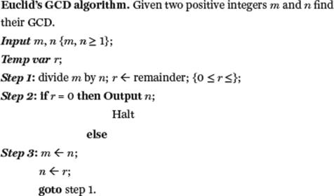
Yet, the concept of an algorithm (if not the word) reaches back to antiquity. Euclid’s great work, Elements (c.300 BCE) where the principles of plane geometry were laid out, described an algorithm to find the greatest common divisor (GCD) of two positive integers. The word ‘algorithm’ itself originated in the name of 9th-century Arabic mathematician and astronomer, Mohammed ibn-Musa al-Khwarizmi, who lived and worked in one of the world’s premier scientific centres of his age, the House of Wisdom in Baghdad. In one of his many treatises on mathematics and astronomy, al-Khwarizmi wrote on the ‘Hindu art of reckoning’. Mistaking this work as al-Khwarizmi’s own, later readers of Latin translations called his work ‘algorismi’ which eventually became ‘algorism’ to mean a step-by-step procedure. This metamorphosed into ‘algorithm’. The earliest reference the Oxford English Dictionary could find for this word is in an article published in an English scientific periodical in 1695.
Donald Knuth (who perhaps more than any other person made algorithms part of the computer scientist’s consciousness) once described computer science as the study of algorithms. Not all computer scientists would agree with this ‘totalizing’ sentiment, but none could conceive of a computer science without algorithms at its epicentre. Much like the Darwinian theory of evolution in biology, all roads in computing seem to lead to algorithms. If to think biologically is to think evolutionarily, to think computationally is to form the habit of algorithmic thinking.
The litmus test
As an entry into this realm, consider the litmus test, which is one of the first experiments a student performs in high school chemistry.
There is a liquid of some unknown sort in a test tube or beaker. The experimenter dips a strip of blue litmus paper into it. It turns red, therefore the liquid is acidic; it remains blue, it is not acidic. In the latter case the experimenter dips a red litmus strip into the liquid. It turns blue, therefore the liquid is alkaline (basic), otherwise it is neutral.
This is a decision procedure chemistry students learn very early in their chemical education, which we can describe in the following fashion:
if a blue litmus strip turns red when dipped into a liquid
then conclude the liquid is acidic
else
if a red litmus strip turns blue when dipped in the liquid
then conclude the liquid is alkaline
else conclude the liquid is neutral
The notation used here will appear throughout this chapter and in some of the chapters that follow, and needs to be explained. In general, the notation if C then S1 else S2, is used in algorithmic thinking to specify decision making of a certain sort. If the condition C is true then the flow of control in the algorithm goes to the segment S1, and S1 will then ‘execute’. If C is false then control goes to S2, and S2 will then execute. In either case, after the execution of the if then else statement control goes to the statement that follows it in the algorithm.
Notice that the experimenter does not need to know anything about why the litmus test works the way it does. She does not need to know what ‘litmus’ actually is—its chemical composition—nor what chemical process occurs causing the change of colour. To carry out the procedure it is entirely sufficient that (a) the experimenter recognizes litmus paper when she sees it; and (b) she can associate the changes of colour with acids and bases.
The term ‘litmus test’ has become a metaphor for a definitive condition or test. And for good reasons: it is guaranteed to work. There will be an unequivocal outcome; there is no room for uncertainty. Moreover, the litmus test cannot go on indefinitely; the experimenter is assured that within a finite amount of time the test will give a decision.
These conjoined properties of the litmus test—a mechanical procedure which is guaranteed to produce a correct result in a finite amount of time—are essential elements characterizing an algorithm.
When is a procedure an algorithm?
For computer scientists, an algorithm is not just a mechanical procedure or a recipe. In order for a procedure to qualify as an algorithm as computer scientists understand this concept, it must possess the following attributes (as first enunciated by Donald Knuth):
Finiteness. An algorithm always terminates (that is, comes to a halt) after a finite number of steps.
Definiteness. Every step of an algorithm must be precisely and unambiguously specified.
Effectiveness. Each operation performed as part of an algorithm must be primitive enough for a human being to perform it exactly (using, say, pencil and paper).
Input and output. An algorithm must have one or more inputs and one or more outputs.
Let us consider Euclid’s venerable algorithm mentioned earlier to find the GCD of two positive integers m and n (that is, the largest positive integer that divides exactly into m and n). The algorithm is described here in a language that combines ordinary English, elementary mathematical notation, and some symbols used to signify decisions (as in the litmus test example). In the algorithm, m and n serve as ‘input variables’ and n also serves as an ‘output variable’. In addition, a third ‘temporary variable’, denoted as r is required. A ‘comment’, which is not part of the algorithm itself is enclosed in ‘{ }’. The ‘←’ symbol in the algorithm is of special interest: it signifies the ‘assignment operation’: ‘b ← a’ means to copy or assign the value of the variable a into b.
Suppose initially m = 16, n = 12. If a person ‘executes’ this algorithm using pencil and paper, then the values of the three variables m, n, r after each step’s execution will be as follows.
As another example, suppose initially m = 17, n = 14. The values of the three variables after each step’s execution will be the following:
In the first example, GCD (16, 12) = 4, which is the algorithm’s output when it halts; in the second example GCD (17, 14) = 1, which the algorithm outputs after it terminates.
Clearly, the algorithm has inputs. Much less obvious is whether the algorithm satisfies the finiteness criterion. There is a repetition or iteration indicated by the goto command which causes control to return to step 1. As the two examples indicate, the algorithm iterates between steps 1 and 3 until the condition r = 0 is satisfied whereupon the value of n is output as the result and the algorithm comes to a halt. The two examples indicate clearly that for these particular pairs of input values for m and n, the algorithm always ultimately satisfies the termination criterion (r = 0) and will halt. However, how do we know whether for other pairs of values it will not iterate forever alternating steps 1 and 3 and never produces an output? (Thus, in that situation, the algorithm will violate both the finiteness and output criteria.) How do we know that the algorithm will always terminate for all possible positive values of m and n?
The answer is that it must be demonstrated that in general, the algorithm is finite. This demonstration lies in that after every test of r = 0 in step 2, the value of r is less than the positive integer n, and the values of n and r decreases with every execution of step 1. A decreasing sequence of positive integers must eventually reach 0 and so eventually r = 0, and so by virtue of step 2 the procedure will eventually terminate.
What about the definiteness criterion? What this says is that every step of an algorithm must be precisely defined. The actions to be carried out must be unambiguously specified. Thus language enters the picture. The description of Euclid’s algorithm uses a mix of English and vaguely mathematical notation. The person who mentally executes this algorithm (with the aid of pencil and paper) is supposed to understand exactly what it means to divide, what a remainder is, what positive integers are. He must understand the meaning of the more formal notation, such as the symbols ‘if … then … else’, ‘goto’.
As for effectiveness, all the operations to be performed must be primitive enough that they can be done in a finite length of time. In this particular case the operations specified are basic enough that one can carry them out on paper as was done earlier.
‘Go forth and multiply’
The concept of abstraction applies to the specification of algorithms. In other words, a particular problem may be solved by algorithms specified at two or more different levels of abstraction.
Before the advent of pocket calculators children were taught to multiply using pencil and paper. The following is what I was taught as a child. For simplicity, assume a three-digit number (the ‘multiplicand’) is being multiplied by a two-digit number (the ‘multiplier’).
Step 1: Place the numbers so that the multiplicand is the top row and the multiplier is the row below and position them so that the units digit of the multiplier is aligned exactly below the units digit of the multiplicand.
Step 2: Draw a horizontal line below the multiplier.
Step 3: Multiply the multiplicand by the units digit of the multiplier and write the result (‘partial product’) below the horizontal line, positioning it so that the units digits are all aligned.
Step 4: Place a ‘0’ below the units digit of the partial product obtained in step 3.
Step 5: Multiply the multiplicand with the tens digit of the multiplier and position the result (partial product) on the second row below the horizontal line to the left of the ‘0’.
Step 6: Draw another horizontal line below the second partial product.
Step 7: Add the two partial products and write it below the second horizontal line.
Step 8: Stop. The number below the second line is the desired result.
Notice that to perform this procedure successfully the child has to have some prior knowledge: (a) She must know how to multiply a multi-digit number by a one-digit number. This entails either memorizing the multiplication table for two one-digit multiplications or having access to the table. (b) She must know how to add two or more one-digit numbers; and she must know how to handle carries. (c) She must know how to add two multi-digit numbers.
However, the child does not need to know or understand why the two numbers are aligned according to step 1; or why the second partial product is shifted one position to the left as per step 5; or why a ‘0’ is inserted in step 4; or why when she added the two partial products in step 7 the correct result obtains.
Notice, though, the preciseness of the steps. As long as someone follows the steps exactly as stated this procedure is guaranteed to work provided conditions (a) and (b) mentioned earlier are met by the person executing the procedure. It is guaranteed to produce a correct result in a finite amount of time: the fundamental characteristics of an algorithm.
Consider how most of us nowadays would do this multiplication. We will summon our pocket calculator (or smart phone), and we will proceed to use the calculator as follows:
Step 1’: Enter the multiplicand.
Step 2’: Press ‘x’.
Step 3’: Enter the multiplier.
Step 4’: Press ‘=’.
Step 5’: Stop. The result is what is displayed.
This is also a multiplication algorithm. The two algorithms achieve the same result but they are at two different levels of abstraction. Exactly what happens in executing steps 1’–4’ in the second algorithm the user does not know. It is quite possible that the calculator is implementing the same algorithm as the paper and pencil version. It is equally possible that a different implementation is used. This information is hidden from the user.
The levels of abstraction in this example also imply levels of ignorance. The child using the paper-and-pencil algorithm knows more about multiplication than the person using a pocket calculator.
The determinacy of algorithms
An algorithm has the comforting property that its performance does not depend on the performer, as long as the knowledge conditions (a)–(c) mentioned earlier are satisfied by the performer. For the same input to an algorithm the same output will obtain regardless of who (or what) is executing the algorithm. Moreover, an algorithm will always produce the same result regardless of when it is executed. Collectively, these two attributes imply that algorithms are determinate.
Which is why cookbook recipes are usually not algorithms: oftentimes they include steps that are ambiguous, thus undermining the definiteness criterion. For example, they may include instructions to add ingredients that have been ‘mashed lightly’ or ‘finely grated’ or an injunction to ‘cook slowly’. These instructions are too ambiguous to satisfy the conditions of algorithm-hood. Rather, it is left to the cook’s intuition, experience, and judgement to interpret such instructions. This is why the same dish prepared from the same recipe by two different cooks may differ in taste; or why the same recipe followed by the same person on two different occasions may differ in taste. Recipes violate the principle of determinacy.
Algorithms are abstract artefacts
An algorithm is undoubtedly an artefact; it is designed or invented by human beings in response to goals or needs. And insofar as they process symbol structures (as in the cases of the GCD and multiplication algorithms) they are computational. (Not all algorithms process symbol structures: the litmus test takes physical entities—a test tube of liquid, a litmus strip—as inputs and produces a physical state—the colour of the litmus strip—as output. The litmus test is a manual algorithm that operates upon physico-chemical entities, not symbol structures; we should not, then, think of it as a computational artefact.)
But algorithms, whether computational or not, themselves have no physical existence. One can neither touch nor hold them, feel them, taste them, or hear them. They obey neither the laws of physics and chemistry nor the laws of engineering sciences. They are abstract artefacts. They are made of symbol structures which, like all symbol structures, represent other things in the world which themselves may be physical (litmus paper, chemicals, buttons on a pocket calculator, etc.) or abstract (integers, operations on integers, relations such as equality, etc.).
An algorithm is a tool. And as in the case of most tools, the less the user needs to know its theoretical underpinnings the more effective an algorithm is for the user.
This raises the following point: as an artefact an algorithm is Janus-faced. (Janus was the Roman god of gates who looked simultaneously in two opposite directions.) Its design or invention generally demands creativity, but its use is a purely mechanical act demanding little creative thought. Executing an algorithm is, so to speak, a form of mindless thinking.
Algorithms are procedural knowledge
As artefacts, algorithms are tools users deploy to solve problems. Once created and made public they belong to the world. This is what makes algorithms objective (as well as determinate) artefacts. But algorithms are also embodiments of knowledge. And being objective artefacts they are embodiments of what philosopher of science Karl Popper called ‘objective knowledge’. (It may sound paradoxical to say that the user of an algorithm is both a ‘mindless thinker’ yet a ‘knowing subject’; but even thinking mindlessly is still thinking, and thinking entails drawing upon knowledge of some sort.) But what kind of knowledge does the algorithm represent?
In the natural sciences we learn definitions, facts, theories, laws, etc. Here are some examples from elementary physics and chemistry.
(i) The velocity of light in a vacuum is 186,000 miles per second.
(ii) Acceleration is the rate of change of velocity.
(iii) The atomic weight of hydrogen is 1.
(iv) There are four states of matter, solid, liquid, gas, and plasma.
(v) When the chemical elements are arranged in order of atomic numbers there is a periodic (recurring) pattern of the properties of the elements.
(vi) Combustion requires the presence of oxygen.
In each case something is declared to be the case: that combustion requires the presence of oxygen; that the atomic weight of hydrogen is 1; that acceleration is the rate of change of velocity; and so on. The (approximation to) truth of these statements is either by way of definition (ii); calculation (i); experimentation or observation (iv, vi); or reasoning (v). Strictly speaking, taken in isolation, they are items of information which when assimilated become part of a person’s knowledge (see Chapter 1). This kind of knowledge is called declarative knowledge or, more colloquially, ‘know-that’ knowledge.
Mathematics also has declarative knowledge, in the form of definitions, axioms, or theorems. For example, a fundamental axiom of arithmetic, due to the Italian mathematician Giuseppe Peano is the principle of mathematical induction:
Any property belonging to zero, and also to the immediate successor of every number that has that property, belongs to all numbers.
Pythagoras’s theorem, in contrast, is a piece of declarative knowledge in plane geometry by way of reasoning (by proof):
In a right-angled triangle with sides a, b forming the right angle and c the hypotenuse, the relationship ![]() is true.
is true.
Here is an example of declarative mathematical knowledge by definition:
The factorial of a non-negative integer n is:
![]()
In contrast, an algorithm is not declarative; rather it constitutes a procedure, describing how to do something. It prescribes action of some sort. Accordingly, an algorithm is an instance of procedural knowledge or, colloquially, ‘know-how’.
For a computer scientist it is not enough to know that the factorial of a number is defined as such and such. She wants to know how to compute the factorial of a number. She wants an algorithm, in other words. For example:
FACTORIAL
Input: n ≥ 0;
Temp variable: fact;
Step 1: fact ➔ 1;
Step 2: if n ≠ 0 and n ≠ 1 then
repeat
Step 3: fact ➔ fact * n;
Step 4: n = n – 1;
Step 5: until n = 1;
Step 6: output fact;
Step 7: halt
The notation repeat S until C specifies an iteration or loop. The statement(s) S will iteratively execute until the condition C is true. When this happens, the loop terminates and control flows to the statement following the iteration.
Here, in step 1, fact is assigned the value 1. If n = 0 or 1, then the condition in step 2 is not satisfied, in which case control goes directly to step 6 and the value of fact = 1 is output and the algorithm halts in step 7. On the other hand if n is neither 1 nor 0 then the loop indicated by the repeat … until segment is iteratively executed, each time decrementing n by 1 until the loop termination condition n = 1 is satisfied. Control then goes to step 6 which when executed outputs the value of fact as ![]() .
.
Notice that the same concept—‘factorial’—can be presented both declaratively (as mathematicians would prefer) and procedurally (as computer scientists would desire). In fact the declarative form provides the underlying ‘theory’ (‘what is a factorial?’) for the procedural form, the algorithm (‘how do we compute it?’).
In summary, algorithms constitute a form of procedural but objective knowledge.
Designing algorithms
The abstractness of algorithms has a curious consequence when we consider the design of algorithms. This is because, in general, design is a goal-oriented (purposive) act which begins with a set of requirements R to be met by an artefact A yet to exist, and ends with a symbol structure that represents the desired artefact. In the usual case this symbol structure is the design D(A) of the artefact A. And the designer’s goal is to create D(A) such that if A is implemented according to D(A) then A will satisfy R.
This scenario is unproblematic when the artefact A is a material one; the design of a bridge, for example, will be a representation of the structure of the bridge in the form of engineering drawings and a body of calculations and diagrams showing the forces operating on the structure. In the case of algorithms as artefacts, however, the artefact itself is a symbol structure. Thus, to speak of the design of an algorithm is to speak of a symbol structure (the design) representing another symbol structure (the algorithm). This is somewhat perplexing.
So in the case of algorithms it is more sensible and rational to think of the design and the artefact as the same. The task of designing an algorithm is that of creating a symbol structure which is the algorithm A such that A satisfies the requirements R.
The operative word here is ‘creating’. Designing is a creative act and, as creativity researchers have shown, the creative act is a complicated blend of reason, logic, intuition, knowledge, judgement, guile, and serendipity. And yet design theorists do talk about a ‘science of design’ or a ‘logic of design’.
Is there, then a scientific component to the design of algorithms? The answer is: ‘up to a point’. There are essentially three ways in which a ‘scientific approach’ enters into the design of algorithms.
To begin with, a design problem does not exist in a vacuum. It is contextualized by a body of knowledge (call it a ‘knowledge space’) relevant to the problem and possessed by the designer. In designing a new algorithm this knowledge space becomes relevant. For instance, a similarity between the problem at hand and the problem solved by an existing algorithm (which is part of the knowledge space) may be discovered; thus the technique applied in the latter may be transferred to the present problem. This is a case of analogical reasoning. Or a known design strategy may seem especially appropriate to the problem at hand, so this strategy may be attempted, though with no guarantee of its success. This is a case of heuristic reasoning. Or there may exist a formal theory relevant to the domain to which the problem belongs; thus the theory may be brought to bear on the problem. This is a case of theoretical reasoning.
In other words, forms of reasoning may be brought to bear in designing an algorithm based on a body of established or well-tried or proven knowledge (both declarative and procedural). Let us call this the knowledge factor in algorithm design.
But, just to come up with an algorithm is not enough. There is also the obligation to convince oneself and others that the algorithm is valid. This entails demonstrating by systematic reasoning that the algorithm satisfies the original requirements. I will call this the validity factor in algorithm design.
Finally, even if it is shown that the algorithm is valid this may not be enough. There is the question about its performance: how good is the algorithm? Let us call this the performance factor in algorithm design.
These three ‘factors’ all entail the kinds of reasoning, logic, and rules of evidence we normally associate with science. Let us see by way of some examples how they contribute to the science of algorithm design.
The problem of translating arithmetic expressions
There is a class of computer programs called compilers whose job is to translate a program written in a ‘high level’ programming language (that is, a language that abstracts from the features of actual physical computers; for example, Fortran or C++) into a sequence of instructions that can be directly executed (interpreted) by a specific physical computer. Such a sequence of machine-specific instructions is called ‘machine code’. (Programming languages are discussed in Chapter 4.)
A classical problem faced by the earliest compiler writers (in the late 1950s and 1960s) was to develop algorithms to translate arithmetic expressions that appear in the program into machine code. An example of such an expression is
![]()
Here, +, −, *, and / are the four arithmetic operators; variables a, b, c, d and the constant number 1 are called ‘operands’. An expression of this form, in which the arithmetic operators appear between its two operands is called an ‘infix expression’.
The knowledge space surrounding this problem (and possessed by the algorithm designer) includes the following rules of precedence of the arithmetic operators:
1. In the absence of parentheses, *, / have precedence over +, −.
2. *, / have the same precedence; +, − have the same precedence.
3. If operators of the same precedence appear in an expression, then left-to-right precedence applies. That is, operators are applied to operands in order of their left-to-right occurrence.
4. Expressions within parentheses have the highest precedence.
Thus, for example in the case of the expression given earlier, the order of operators will be:
a. Perform a + b. Call the result t1.
b. Perform 1/d. Call the result t2.
c. Perform c – t2. Call the result t3.
d. Perform t1 * t3.
On the other hand if the expression was parenthesis-free:
![]()
then the order of operators would be:
i. Perform b * c. Call the result t1’.
ii. Perform 1/d. Call the result t2’.
iii. Perform a + t1’. Call the result t3’.
iv. Perform t3’ – t2’.
An algorithm can be designed to produce machine code which when executed will correctly evaluate infix arithmetic expressions according to the precedence rules. (The precise nature of the algorithm will depend on the nature of the machine-dependent instructions, an idiosyncracy of the specific physical computer.) Thus the algorithm, based on the precedence rules, draws on precise rules that are part of the knowledge space relevant to the problem. Moreover, because the algorithm is based directly on the precedence rules, arguing for the algorithm’s validity will be greatly facilitated. However, as the earlier examples show, parentheses make the translation of an infix expression somewhat more complicated.
There is a notation for specifying arithmetic expressions without the need for parentheses, invented by the Polish logician Jan Lukasiewiz (1878–1956) and known, consequently, as ‘Polish notation’. In one form of this notation, called ‘reverse Polish’, the operator immediately follows its two operands in a reverse Polish expression. The following examples show the reverse Polish form for a few infix expressions.
a. For a + b the reverse Polish is a b +.
b. For a + b − c the reverse Polish is a b + c −.
c. For a + b * c the reverse Polish is a b c * +.
d. For (a + b)* c the reverse Polish is a b + c *.
The evaluation of a reverse Polish expression proceeds left-to-right in a straightforward fashion, thus making the translation problem easier. The rule is that the arithmetic operators encountered are applied to their preceding operands in the order of the appearance of the operators, left-to-right. For example, in the case of the infix expression
![]()
the reverse Polish form is
![]()
and the order of evaluation is:
i. Perform a b + and call the result t1. So the resulting expression is t1 c 1 d/ − *.
ii. Perform 1 d/and call the result t2. So the resulting expression is t1 c t2 − *.
iii. Perform c t2 − and call the result t3. So the resulting expression is t1 t3 *.
iv. Perform t1 t3 *.
Of course, programmers will write arithmetic expressions in the familiar infix form. The compiler will implement an algorithm that will first translate infix expressions into reverse Polish form and then generate machine code from the reverse Polish expressions.
The problem of converting infix expressions to reverse Polish form illustrates how a sound theoretical basis and a proven design strategy can combine in designing an algorithm that is provably correct.
The design strategy is called recursion, and is a special case of a broader problem solving strategy known as ‘divide-and-rule’. In the latter, given a problem P, if it can be partitioned into smaller subproblems p1, p2, … , pn, then solve p1, p2, … , pn independently and then combine the solutions to the subproblems to obtain a solution for P.
In recursion, the problem P is divided into a number of subproblems that are of the same type as P but smaller. Each subproblem is divided into still smaller subproblems of the same type and so on until the subproblems become small and simple enough to be solved directly. The solutions of the subproblems are then combined to give solutions to the ‘parent’ subproblems, and these combined to form solutions to their parents until a solution to the original problem P obtains.
Consider now the problem of converting algorithmically infix expressions into reverse Polish expressions. Its basis is a set of formal rules:
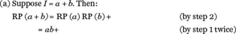
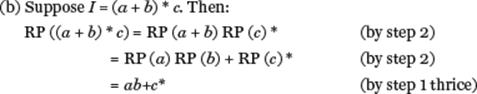
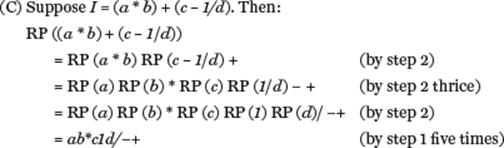
Let B = {+, −, *, /} be the set of binary arithmetic operators (that is, each operator b in B has exactly two operands). Let a denote an operand. For an infix expression I denote by I’ its reverse Polish form. Then:
(a) If I is a single operand a the reverse Polish form is a.
(b) If I1 b I2 is an infix expression where b is an element of B, then the corresponding reverse Polish expression is I1’ I2’ b.
(c) If (I) is an infix expression its reverse Polish form is I’.
The recursive algorithm constructed directly from these rules is shown later as a function—in the mathematical sense of this term. In mathematics, a function F applied to an ‘argument’ x, denoted Fx or F(x), returns the value of the function for x. For example, the trigonmetric function SIN applied to the argument 90 (degrees), denoted as SIN 90, returns the value 1. The square root function symbolized as √ applied to an argument, say 4 (symbolized as √4), returns the value 2.
Accordingly, the algorithm, named here RP with an infix expression I as argument is as follows.
RP (I)
Step 1: if I = a then return a
else
Step 2: if I = I1 b I2
then return RP (I1) RP (I2) b
else
Step 3: if I = (I1) then return RP (I1)
Step 4: halt
Step 3, of the general form if C then S is a special case of the if then else decision form: control flows to S only if condition C is true, otherwise control flows to the statement that follows the if then.
The function RP can thus activate itself recursively with ‘smaller’ arguments. It is easily seen that RP is a direct implementation of the conversion rules and so, is correct by construction. (Of course, not all algorithms are so self-evidently correct; their theoretical foundation may be much more complex and their correctness must then be demonstrated by careful argument or even some form of mathematical proof; or their theoretical basis may be weak or even non-existent.)
To illustrate how the algorithm works with actual arguments, consider the following examples.
The ‘goodness’ of algorithms as utilitarian artefacts
As mentioned before, it is not enough to design a correct algorithm. Like the designer of any utilitarian artefact the algorithm designer must be concerned with how good the algorithm is, how efficiently it does its job. Can we measure the goodness of an algorithm in this sense? Can we compare two rival algorithms for the same task in some quantitative fashion?
The obvious factor of goodness will be the amount of time the algorithm takes to execute. But an algorithm is an abstract artefact. We cannot measure it in physical time; we cannot measure time on a real clock since an algorithm qua algorithm does not involve any material thing. If I as a human being execute an algorithm I suppose I could measure the amount of time I take to perform the algorithm mentally (perhaps with the aid of pencil and paper). But that is only a measure of my performance of the algorithm on a specific set of input data. Our concern is to measure the performance of an algorithm across all its possible inputs and regardless of who is executing the algorithm.
Algorithm designers, instead, assume that each basic step of the algorithm takes the same unit of time. Think of this as ‘abstract time’. And they conceive the size of a problem for which the algorithm is designed in terms of the number of data items that the problem is concerned with. They then adopt two measures of algorithmic ‘goodness’. One has to do with the worst case performance of the algorithm as a function of the size n of the problem; the other measure deals with its average performance, again, as a function of the problem size n. Collectively, they are called time complexity. (An alternative measure is the space complexity: the amount of (abstract) memory space required to execute the algorithm.)
The average time complexity is the more realistic goodness measure, but it demands the use of probabilities and is, thus, more difficult to analyse. In this discussion we will deal only with the worst case scenario.
Consider the following problem. I have a list of n items. Each item consists of a student name and his/her email address. The list is ordered alphabetically by name. My problem is to search the list and find the email address for a particular given name.
The simplest way to do this is to start at the beginning of the list, compare each name part of each item with the given student name, proceed along the list one by one until a match is found, and then output the corresponding email address. (For simplicity, we will assume that the student’s given name is somewhere in the list.) We call this the ‘linear search algorithm’.
LINEAR SEARCH
Input: student: an array of n entries, each entry consisting of two ‘fields’, denoting name (a character string) and email (a character string) respectively. For the i-th entry in student, denote the respective fields by student [i].name and student[i].email.
Input: given-name: the name being ‘looked up’.
Temp variable i: an integer
Step 1: i ← 1;
Step 2: while given-name ≠ student[i].name
Step 3: do i ← I + 1;
Step 4: output student[i].email
Step 5: halt
Here, the generic notation while C do S specifies another form of iteration: while the condition C is true repeatedly execute the statement (‘loop body’) S. In contrast to the repeat S until C, the loop condition is tested before the loop body is entered on each iteration.
In the worst possible case the desired answer appears in the very last (n-th) entry. So, in the worst case scenario, the while loop will be iterated n times. In this problem n, the number of students in the list, is the critical factor: this is the problem size.
Suppose each step takes roughly the same amount of time. In the worst case, this algorithm needs 2n + 3 time steps to find a match. Suppose n is very large (say 20,000). In that case, the additional factor ‘3’ is negligible and can be ignored. The multiplicative factor ‘2’ though doubling n is a constant factor. What dominates is n, the problem size; it is this that might vary from one student list to another. We are interested, then, in saying something about the goodness of the algorithm in terms of the amount of (abstract) time needed to perform the algorithm as a function of this n.
If an algorithm processes a problem of size n in time kn, where k is a constant, we say that the time complexity is of order n, denoted as O(n). This called the Big O notation, introduced by a German mathematician P. Bachmann in 1892. This notation gives us a way of specifying the efficiency (complexity) of an algorithm as a function of the problem size. In the case of the linear search algorithm, its worst case complexity in O(n). If an algorithm solves a problem in the worst case in time kn2, its worst case time complexity is O(n2). If an algorithm takes time knlogn its time complexity is O(nlogn), and so on.
Clearly, then, for the same problem of size n an O(logn) algorithm will need less time than an O(n) algorithm, which will need less time than an O(nlogn) algorithm, and the latter will need less time than an O(n2) algorithm; the latter will be better than an O(n3) algorithm. The worst algorithms are those whose time complexity is an exponential function of n, such as an O(2n) algorithm. The differences in the goodness of algorithms with these kinds of time complexities, were starkly illustrated by computer scientists Alfred Aho, John Hopcroft, and Jeffrey Ullman in their influential text The Design and Analysis of Algorithms (1974). They showed that, assuming a certain amount of physical time to perform steps of an algorithm, in 1 minute an O(n) algorithm could solve problems of size n = 6 * 104; an O(nlogn) algorithm for the same problem could solve problems of size n = 4,893; an O(n3) algorithm solves the same problem but only of size n = 39; and an exponential algorithm of O(2n) could only solve the problem of size n = 15.
Algorithms can thus be placed in a hierarchy based on their Big O time complexity, with an O(k) algorithm (where k is a constant) highest in the hierarchy and exponential algorithms of O(kn) lowest. Their goodness drops markedly as one proceeds down the hierarchy.
Consider the student list search problem, but this time taking into account the fact that the entries in the list are alphabetically ordered by student name. In this one can do what we approximately do when searching a phone book or consulting a dictionary. When we look up a directory we don’t start from page one and look up each name one at a time. Instead, supposing the word whose meaning we seek in a dictionary begins with a K. We flip the pages of the dictionary to one that is roughly near the Ks. If we open the dictionary to the Ms, for example, we know we have to flip back; if we open at the Hs we have to flip forward. Taking advantage of the alphabetic ordering we reduce the amount of search.
This approach can be followed more exactly by way of an algorithm called binary search. Assuming the list has k = 2n − 1 entries, in each step the middle entry is identified. If the student name so identified is alphabetically ‘lower’ than the given name, the algorithm will ignore the entries to the left of the middle element. It will then identify the middle entry of the right half of the list and again compare. Each time, if the name is not found, it will halve the list again and continue until a match is found.
Suppose that the list has k = 15 (i.e. 24 − 1) entries. And suppose these are numbered 1 through 15. Then it can easily be confirmed that the maximum paths the algorithm will travel will be one of the following:
8 ➔ 4 ➔2 ➔1
8 ➔ 4 ➔ 2 ➔ 3
8 ➔ 4 ➔ 6 ➔ 5
8 ➔ 4 −➔ 6 ➔ 7
8 ➔ 12 ➔ 10 ➔ 9
8 ➔ 12 ➔ 10 ➔ 11
8 ➔ 12 ➔ 14 ➔ 13
8 ➔ 12 ➔ 14 ➔ 15
Here, the list entry 8 is the middle entry. So, at most only 4 = log216 entries will be searched before a match is found. For a list of size n the worst case performance of binary search is O (log n), an improvement over the linear search algorithm.
The aesthetics of algorithms
The aesthetic experience—the quest for beauty—is found not only in art, music, film, and literature but also in science, mathematics, and even technology. ‘Beauty is truth, truth beauty’, began the final lines of John Keats’s Ode on a Grecian Urn (1820). The English mathematician G.H. Hardy, echoing Keats, roundly rejected the very idea of ‘ugly mathematics’.
Consider why mathematicians seek different proofs for some particular theorem. Once someone has discovered a proof for a theorem why should one bother to find another, different, proof? The answer is that mathematicians seek new proofs of theorems when the existing ones are aesthetically unappealing. They seek beauty in their mathematics.
This applies just as much to the design of algorithms. A given problem may be solved by an algorithm which is, in some way, ugly—that is, clumsy, or plodding. Sometimes this is manifested in the algorithm being inefficient. So computer scientists, especially those who have a training in mathematics, seek beauty in algorithms in exactly the same sense that mathematicians seek beauty in their proofs. Perhaps the most eloquent spokespersons for an aesthetics of algorithms were the computer scientists Edsger Dijkstra from the Netherlands, C.A.R. Hoare from Britain, and Donald Knuth from the United States. As Dijkstra once put it, ‘Beauty is our business’.
This aesthetic desire may be satisfied by seeking algorithms being simpler, more well structured, or using a ‘deep’ concept.
Consider, for example, the factorial algorithm described earlier in this chapter. This iterative algorithm was based on the definition of the factorial function as:
![]()
But there is a recursive definition of the factorial function:
![]()
The corresponding algorithm, as a function, is:
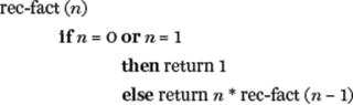
Many computer scientists would find this a more aesthetically appealing algorithm because of its clean, easily understandable, austere form and the fact that it takes advantage of the more subtle recursive definition of the factorial function. Notice that the recursive and the non-recursive (iterative) algorithms are at different levels of abstraction: the recursive version might be implemented by some variant of the non-recursive version.
Intractable (‘really difficult’) problems
I end this chapter by shifting focus from algorithms that solve computational problems to the computational problems themselves. In an earlier section we saw that the performance of algorithms can be estimated in terms of their time (or space) complexity. For example, in the case of the student list search problem the two algorithms (linear search and binary search), though solving the same problem manifested two different worst case time complexities.
But consider the so-called ‘travelling salesman problem’: Given a set of cities and road distances between them, can a salesman beginning at his base city visit all the cities and return to his origin such that the total distance travelled is less than or equal to some particular value? As it happens, there is no known algorithm for this problem that is less than of exponential time complexity (O(kn), for some constant k and problem size n (such as the number of cities)).
A computational problem is said to be intractable—‘really difficult’—if all the known algorithms to solve the problem are of at least exponential time complexity. Problems for which there exist algorithms of polynomial time complexity (e.g. O(nk)) are said to be tractable—that is, ‘practically feasible’.
The branch of computer science that deals with the in/tractability of computational problems is a formal, mathematical domain called the theory of computational complexity, founded in the 1960s and early 1970s predominantly by the Israeli Michael Rabin, the Canadian Stephen Cook, and the Americans Juris Hartmanis, Richard Stearns, and Richard Karp.
Complexity theorists distinguish between two problem classes called P and NP, respectively. The formal (that is, mathematical) definitions of these classes are formidable, related to automata theory and, in particular, certain kinds of Turing machines (see Chapter 2), and they need not detain us here. Informally, the class P consists of all problems solvable in polynomial time—and these are, thus tractable. Informally, the class NP consists of problems for which a proposed solution, which may or may not be obtained in polynomial time, can be checked to be true in polynomial time. For example, the travelling salesman problem does not have a (known) polynomial time algorithmic solution but given a solution it can be ‘easily’ checked in polynomial time whether the solution is correct.
But, as noted, the travelling salesman problem is intractable. Thus, the NP class may contain problems believed to be intractable—although NP also contains the P class of tractable problems.
The implications of these ideas are considerable. Of particular interest is a concept called NP-completeness. A problem π is said to be NP-complete if π is in NP and all other problems in NP can be transformed or reduced in polynomial time to π. This means that if π is intractable then all other problems in NP are intractable. Conversely, if π is tractable, then all other problems in NP are also tractable. Thus, all the problems in NP are ‘equivalent’ in this sense.
In 1971, Stephen Cook introduced the concept of NP-completeness and proved that a particular problem called the ‘satisfiability problem’ is NP-complete. (The satisfiability problem involves Boolean (or logical) expressions—for example the expression (a or b) and c, where the terms a, b, and c are Boolean (logical) variables having only the possible (truth) values TRUE and FALSE. The problems asks: ‘Is there a set of truth values for the terms of a Boolean expression such that the value of the expression is TRUE?’) Cook proved that any problem in NP can be reduced to the satisfiability problem which is also in NP. Thus, if the satisfiability problem is in/tractable then so is every other problem in NP.
This then raised the following question: Are there polynomial time algorithms for all NP problems? We noted earlier that NP contains P. But what this question asks is: Is P identical to NP? This is the so-called P = NP problem, arguably the most celebrated open problem in theoretical computer science. No one has proved that P = NP, and it is widely believed that this is not the case; that is, it is widely believed (but not yet proved) that P ≠ NP. This would mean that there are problems in NP (such as the travelling salesman and the satisfiability problems) that are not in P, hence are inherently intractable; and if they are NP-complete then all other problems reducible to them are also intractable. There are no practically feasible algorithms for such problems.
What the theory of NP-completeness tells us is that many seemingly distinct problems are connected in a strange sort of way. One can be transformed into another; they are equivalent to one another. We grasp the significance of this idea once we realize that a huge range of computational problems applicable in business, management, industry, and technology—‘real world’ problems—are NP-complete: if only one could construct a feasible (polynomial time) algorithm for one of these problems, one could find a feasible algorithm for all the others.
So how does one cope with such intractable problems? One common approach is the subject of Chapter 6.