Total Information Risk Management (2014)

PART 3 Total Information Risk Management Techniques

CHAPTER 12 Software Tools

Automated Methods for TIRM

Abstract

This chapter shows how automated software solutions can support the TIRM process and mitigate information risks.

Keywords

Software Tools; InfoRAS; Data Profiling; Domain Analysis; Primary and Foreign Key Analysis; Matching Algorithms; Lexical Analysis and Validation; Automated Information Flow Discovery; Master Data Management (MDM)

What you will learn in this chapter

How to automate some of the TIRM process stages

What information management tools and technologies are currently available for detecting and mitigating information risks

Introduction

The vast amount of information that an organization collects on an almost daily basis offers a wide range of new opportunities that can be leveraged to increase an organization’s decision-making capability. The automation of business processes has led to a vast increase in the amount of information captured and used throughout organizations. This already immeasurable amount of information from within the various departments and business units is being augmented with rich data sets sourced externally from resources as diverse as social networks, publicly available government data, and partner organizations. For example, smartphones have the capability to connect to the web and facilitate the upload of information to core organizational information systems about events as they happen. Wireless sensors provide continuous streams of operational data, and integration technologies like virtualization can extract and present data from millions of websites, including social networks, directly to the operational staff.

The challenge posed by the availability of all of this data is the speed at which organizations need to operate to make effective use of it. Automating the management of this data in today’s overflowing and information-rich environment is critical. Automation within the TIRM process is no exception. Leading managers must consider the ways in which automation of the relevant steps in the TIRM process can save time and ensure an accurate output.

There are a number of available software tools that can be used to support the automation of various TIRM steps. The following sections describe how the steps of understanding the information environment, identifying the information quality problems during task execution, and the information risk assessment stage of the TIRM process can be supported with such tools. Automating the TIRM steps is only one part of the story. The other part is concerned with the identification of technologies that need to be applied to help mitigate the risks that are posed by information errors. The final section of this chapter, therefore, provides two example cases of information risks and how these can be mitigated with the aid of automated information management technologies and their associated architectures.

Automating the understanding the information environment step

Investigating the information environment in the TIRM process involves creating a register of the information resources that are in the scope of the project under consideration. These could be resources such as databases, electronic or paper-based documents, ERP systems, spreadsheets, etc. With this as a basis, it is necessary to identify the type of information in each system, categories how this information flows within and between these systems, and document any known quality issues.

First, the type of information is an important concept to capture, because it not only dictates how it is to be used, but it also indicates the types of problems that are likely to occur, as well as the types of automated information management technologies that will be appropriate to mitigate these problems. There are four main categories of organizational information: master data, transactional data, reference data, and metadata. The first two categories are described together because of their linkages.

Master and transactional data

Transactional data relates to the transactions of the organization and includes data that is captured, for example, when a product is sold or purchased. Master data is referred to in different transactions, and examples are customer, product, or supplier data. Generally, master data does not change and does not need to be created with every transaction. For example, if one customer purchases multiple products at different times, a transaction record needs to be created for each sale, but the data about the customer stays the same. Figure 12.1 shows how master data forms part of a transactional record. In this case, when the lamp and chair products are sold, the transaction references the relevant product IDs and customer IDs. The product and customer records, if they already exist, do not need to be recreated or modified for this new transaction. The other data in the transaction, such as the unique identifier for the transaction (i.e., sale ID) and sale time do, however, need to change. Transaction data is therefore typically more volatile than master data as it is created and changes more frequently. Note that this simple example shows the actual sale price in the transaction and price of the product in the master data. There are different ways to model this, but the example shows that the actual price can change depending on the transaction and it may only be calculated from the product price in the master data (after including discounts, etc.). Transaction 003 in Figure 12.1 shows that a discount has been applied to the retail price.

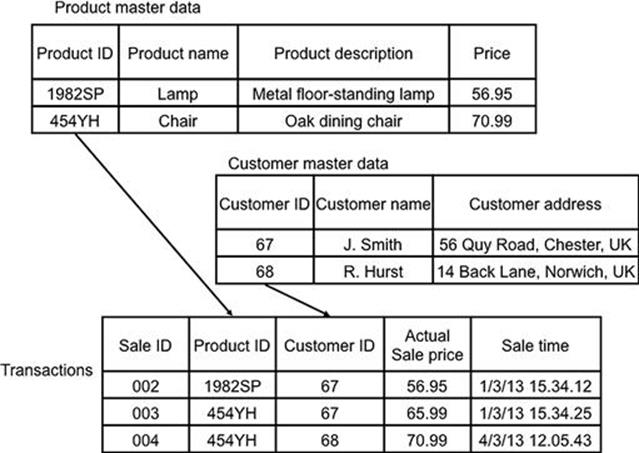
FIGURE 12.1 Master and transactional data.

Another property of master data is that it is often shared and used by different business units. For example, a customer record will be used by marketing as well as sales. Problems arise when one business unit updates the master record and does not inform the other business unit. For example, the marketing department could update the address of a customer and, if they do not inform the sales department, orders could be sent to an out-of-date address.

Although these are the general properties of master and transactional data, there are occasions when these data types behave differently and, thus, this distinction becomes blurred. For example, master data can also appear to be transactional when changes to a supplier address, for instance, are not overwritten in a record, but instead a new record is created. An organization may choose to retain all previous addresses of a supplier, especially if they wish to analyze a supplier’s movement. It is worth paying attention to cases such as these, because it may be better to apply transactional solutions to the problems in this data type so that it is managed correctly.

ACTION TIP

Do not always assume that master data needs to be treated with only master data–related solutions, especially if the master data behaves like transactional data.

When considering the information environment for the TIRM process, transactional data is often found in data warehouses and point-of-sale systems where the transactions occur. Master data is often found in customer relationship management (CRM) software, product life-cycle management (PLM) software, and supplier relationship management (SRM) systems. However, it can also be identified by tracking back from transactional records that refer to customers, products, suppliers, etc. If you find that the only source of the master data is stored in the transactional record, then this is a prime place to look for information risks that may arise from faulty master data.

ACTION TIP

If you find that the only source of the master data is stored in the transactional record, then this is a prime place to look for information risks that may arise from faulty master data.

Reference data

One common problem in business systems is that information is not always entered into the systems consistently. For example, in a supplier table, a field such as “country” could contain many inconsistent values for different suppliers. The problem is that there are many ways of referring to one country. For example, some records could refer to the United Kingdom as GB, UK, Great Britain, or United Kingdom. Reference data is used to address this problem by providing a global reference of standardized and allowable values. Reference data can be best thought of as clarification data because, as the name suggests, it clarifies and expands on the data in transactional and master records. For the supplier country problem, reference data would define the allowable domain of values for each country and would give a clear indication of the real-world entity that each value refers to (Table 12.1 is an example). Reference data is often used in instances where there are codes (such as country codes) or numeric codes that help to reduce storage requirements and make expanded concepts more concise. When arbitrary numeric codes are used, reference data is essential to define the real meaning.

IMPORTANT

Reference data can be best thought of as clarification data because, as the name suggests, it clarifies and expands on the data in transactional and master records.

Table 12.1

Reference Data for Country Codes

Reference data may be managed internally or could reference externally managed codes. For example, the International Organization of Standards (ISO) has a standard that defines country codes (ISO 3166-1) that could be reused in different organizational information systems. Using external codes relieves an organization of the job of managing them, but the disadvantage is that there will be less control over managing changes to the values. It is worth noting that reference data changes infrequently in contrast to master and transactional data.

When investigating the information environment for the TIRM process, reference data can be found in the actual databases as lookup tables. Some database vendors provide options to specify domains of values (or lookup values) within the database management software, and database administrators will know where to find these values. Also, ask the users about where they are constrained (e.g., dropdown lists) when entering values into fields in the applications they use; this can indicate the use of reference data. Note that if you cannot find the reference data, at this stage it would be unwise to start to introduce reference data in places where you would expect to find it. Use data profiling (described later) as a final check to determine if there is a need for reference data in these places.

It is possible to partially automate the discovery and validation of reference data. Column analysis, which is one of the automated methods in data profiling tools, can be applied to identify what values appear for a particular field. Domain analysis can be used to check whether the values in a field match those in the domain. Another option is to cross-check the values used in different databases to see if consistent codes are used; again data profiling tools can be used to support this. Both column and domain analysis are described later in this chapter.

ACTION TIP

If you cannot find the reference data, use data profiling column analysis to identify areas where it may need to be introduced.

Metadata

Metadata is broadly defined as data that describes other data. There are two clear categories of metadata that are important to distinguish: metadata about the operational (actual) data in the system (sometimes referred to as business metadata) and metadata about the system structure (also referred to as technical metadata). Metadata about the actual data in the system includes items such as when and who created or updated the data; how the data was calculated, aggregated, or filtered; and what the quality of the data is. The metadata about the system includes the data model—that is, the details of the structures inside databases and data types used.

It is important to make the distinction between these categories of metadata because of the way in which they are used. The metadata about the actual data is used operationally by the users of an organization’s information system in their daily work. For example, if purchases above a certain amount need to be authorized before they are sent out, the operational staff need to know how the final amount is calculated (e.g., is it the gross amount or net amount, and does it include shipping) before they can assess whether it is above a certain threshold and require authorization.

The structural metadata is not needed for operational tasks but is closer to the design of the system. Clearly, the system needs to be well designed and suitable for the users for the operational work to be successful, but the structural metadata is not needed directly for operational purposes. Database administrators will be able to identify and report what the structural metadata is.

When data needs to be transferred from one system to another (e.g., to a data warehouse), then extract, transform, and load (ETL) operations are used for this purpose. The extract step extracts the data from the source’s system. The transform step is needed to convert the data into a form that is suitable for the target system (because the source and target systems will often have significant variations). Finally, the load step is used to push the data into the target system. Knowing both the operational and structural metadata is essential if ETL is to be a success. For instance, if the field names between the source and target databases are different, then the mapping between the different fields needs to be specified in the transform step so that the data goes to the correct place. Note that two databases may have the same fields (with the same names) but have different meanings—the field “total” could be in two systems, but could mean the gross total in one system and the net total in another system. The data about the operational data is, therefore, also needed to determine how the actual totals have been calculated and whether they are semantically equivalent or not.

The fact that data may have been moved from one system to another via ETL (or other data synchronization techniques) is an important piece of operational metadata to capture: it informs the users of the reliability of the data (i.e., that it has probably been subject to an automated transformation that may not have been verified). This is also referred to as data lineage, which defines where and how information was created—where it flows to, and how it was transformed as it is passed from system to system within the organization.

When understanding the information environment for the TIRM process, identify the two types of metadata that relate to the systems of interest. For the structural metadata, speak to the IT personnel such as database administrators. For the operational metadata, first speak to the users and then the IT personnel. Both of these groups of people should know what is really happening to the data, and their thoughts should be aligned. If not, then this is a prime place that could be causing information risks. In particular, as shown in the previous example, there could be situations where purchases are not being correctly authorized before being sent out, through misunderstandings in the data and the ways it is transformed.

Automated information flow discovery

Information flow refers to the path the information takes while it is being used for a business process. Information may be created in one system, then transferred to another system, modified in that system, then merged with other data, and so on. Be cognizant that the flow of information may be more complex than the business process because there may be multiple information systems and multiple actors using the information in a single business step.

ATTENTION

The flow of information may be more complex than the business process because there may be multiple information systems and multiple actors using the information in a single business step.

New research has emerged that shows a promising approach to help automate the discovery of information flow (Gao et al., 2010). Even more than just automation, it aims to discover what is really happening to the data, and not what users say is happening to it (which may not always be correct). The approach relies on using database log files to see when, what, and where data is being created, read, updated, and deleted. However, this approach is still in the research phase, and therefore, there are no current commercial tools available to support this. It may not be a practical solution for many organizations. That said, organizations with the relevant capabilities in place might want to investigate this further.

The idea of the research is to inspect the information system logs and observe when a data item was created, read, updated, and deleted, and then piece these actions together to gain an overall picture of what is happening to the data. For example, a simple insert statement into a database could indicate that a new product has been created, a new customer has been registered, or a request to purchase a new product has been made. Insert statements are good candidates for indicating the start of a process or when data has been transferred to another system. Also, whether the insert statements are for transactional data or for master data, they can help with the overall understanding of the process.

As an example of this approach, you can see how the following statements, recorded in different system log files, map to the business process in Figure 12.2.

1. [1023] (02/06 09:14:22:57.260): Performing INSERT INTO partRequests (partNumber, requestor, supplierName, totalNet, …) VALUES (…)

2. [1024] (02/06 09:14:25:34.420): Performing SELECT partNumber, requestor, supplierName, totalNet FROM partRequests WHERE totalNet>100

3. [25423] (02/06 09:14:26:15.130): Performing INSERT INTO requestReviews (requestID, partNumber, requestor, supplierName, totalNet) VALUES (<values from query 2>)

4. [25425] (02/06 09:14:45:12.543): Performing UPDATE requestReviews SET approved=true WHERE requestID=“43”

5. [25426] (02/06 09:15:00:05.103): Performing SELECT partNumber, requestor, supplierName, totalNet FROM requestReviews WHERE approved=true

6. [562983] (02/06 09:15:01:14.330): Performing INSERT INTO orders (POnumber, PODate, supplierName, totalNet, …) VALUES (<values from query 5>))

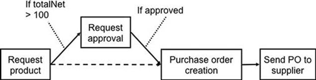
FIGURE 12.2 An example of information flow.

Initially, the part request (in this example this refers to an engineering part that the organization is procuring) is created by inserting a record into the partRequests database (query 1). Queries 2 and 3 show an ETL process where data is taken from the partRequeststable and entered into the requestReviews table in another data source. In addition, it is possible to observe a business rule that determines what data is to be transferred in query 2: when the totalNet value is greater than 100, the data is moved to a system that requires the purchase to be approved. By observing other queries that select this data, it would be possible to determine in what other conditions the data is transferred to other systems. For example, one may observe that all part requests that have a totalNet below 100 may go straight to the purchase ordering system (see the dashed line in Figure 12.2). The update statement in query 4 shows that the user has clarified part of the data by approving the part request. Note that there would most likely be a select statement before the update statement, but it is not necessary to consider this in this specific example. In general, there will be many log file entries that are irrelevant and do not help the process of determining information flow. The challenge is, therefore, to extract the entries that provide the most valuable information.

Queries 5 and 6 show another ETL process that moves the data to the purchase ordering system and creates the purchase order for the part. After this, one would expect to find other log file entries that show the purchase order being sent out, especially in the case where it is transferred electronically.

Note that the timestamps are needed to determine the correct sequence of actions, and it is often the case that timestamps from multiple systems will not be in synchronization. In this case, it is necessary to determine the offset of the timestamps (i.e., the difference in time) between each system and use this to determine what actions occur simultaneously.

Bear in mind that in simple cases, it is often faster to speak to the people involved with the business process, but in more complex scenarios where the data is integrated from multiple systems and it is not easy to establish what happens in every case, log files can provide an invaluable source of reference for what is really happening.

Furthermore, if common groups of operations can be used to determine an information flow scenario, such as an ETL process or business rule being applied, then software to detect and extract these patterns can be developed to automate the process. In this example, there are two ETL processes and these were indicated by a select action from one database and an insert action into another, where the data is similar and the timestamps are close. A rule that governs where the data moves can also be observed in the WHEREclause of query 2.

When investigating the information environment for the TIRM process, use your knowledge of transactional data, master data, reference data, and metadata to help you categorize and understand what is really happening to the data and why it is occurring.

Identify information quality problems during task execution

As part of TIRM, after examining the information resources that are used within the different business processes, it is necessary to identify the actual information quality problems within these resources. The vast quantity of data in many business information systems makes this task extremely challenging and infeasible to conduct manually in many cases. Tools that can automate the discovery of data characteristics within large data sets have already been developed, and these characteristics can give a good indication about whether the data set contains information quality problems. Data profiling tools, the commonly used name for these types of tools, can be used to build a report about the data that shows very detailed statistics about the characteristics of the data.

The limitation of data profiling tools, however, is that, when directed to a particular data set, they do not directly report all the information quality problems in a way that managers can easily digest and understand. Instead, they operate the other way around: an analyst is needed to specify what statistic needs to be known about the data, and the tool will calculate this statistic based on the data set. Therefore, the tools do not directly report what data is inaccurate. The analysts, therefore, need to know what they are looking for, and should carefully report their statistics in a way that can be interpreted by managers and operational staff as meaningful information quality problems.

The following sections describe the different types of analysis that data profiling tools can perform automatically and how these can be interpreted to determine whether information quality problems exist.

Column analysis

Column analysis refers to the different types of statistics that can be gathered from all values within a column of a database table, otherwise referred to as database fields or attributes. If “DateOfBirth” is chosen for the analysis, then data values for the “PostCode” field will not be analyzed (Table 12.2).

Table 12.2

Typical Table Structure

Various measures can be obtained using column analysis, such as the frequency with which each value occurs, the number of unique values, the number of missing values, and standard statistics (maximum, minimum, mean, median, and standard deviation) for numeric values. For example, for the PostCode field a frequency analysis would indicate that CB3 0DS occurs twice and all the other values (including the missing value) occur once. The number of unique values for PostCode is two and there is one missing value for this field. An analysis of the format of the values in a column can be used to identify possible erroneous values. For instance, it is possible to check all the dates in the DateOfBirth column against the formats mm/dd/yyyy and mm/dd/yy. This would indicate that all except the last value match this format in Table 12.2. Similarly, postcodes have predefined formats that can be used to check the postcodes values for errors. Furthermore, especially with numeric data, inaccurate outliers can be identified, while performing a sanity check on the distribution can help to see if there is any suspicious skewing of the data.

EXAMPLE

A car insurance company may know that their customers are mostly between 17 and 27 years old (if they specialize in providing insurance coverage for inexperienced drivers). You may expect to find a small number of people who start driving at an older age, but the distribution should be skewed toward, and truncated at, 17 years old.

One of the best ways to identify problems using a column analysis is to inspect outlying values for the various statistics. For example, if there is only one value that is far from the mean of a range of numeric values, then this is a good candidate to check for an error. Similarly, looking at the values that occur infrequently can help identify problems such as spelling errors and values that have not been formatted consistently. Conversely, excessive use of inaccurate default values (i.e., values that are entered by default by the system and the user does not change them to the correct value) can be spotted by inspecting the very frequent values occurring in a column.

When databases are developed, the data type that will appear in a column is specified as part of the data model (metadata about the system). Types include dates, numeric values, alphanumeric (or string) values, etc. This type may not always match the actual data that is contained within the column when it is used on a day-to-day basis. For example, a field that is defined as a string type could be used to record date values, and a variety of date formats may result, along with text descriptions of dates (e.g., “1950s”). This problem may also occur when data is transferred from one system to another and the data ends up in the wrong column; erroneous ETL operations are one example where this may occur. ETL operations also need to double-check the “real” type of the column data to ensure that it can be successfully loaded into another system without mismatches (a date value will not enter correctly into a numeric field). A column analysis could be used to infer the data type by inspecting each actual value for the column, and therefore detect when there are mismatches between the recorded type and the actual type of data.

Using a column analysis can help to indicate whether reference data is needed: if there are many inconsistent values between different records for a particular field, then it could mean that the users are given too much freedom to enter any value they wish. When addressing this problem, speak to the users of the system and, with their assistance, develop a thorough domain of values that they can choose from to enter into the field.

IMPORTANT

Guard against the problem where the users cannot find the exact entry they need. This results in the situation where the users leave the default value in place or they select the first value in the list. You can detect this by using a column analysis to count the frequency of these values to determine any abnormalities.

ACTION TIP

After introducing a new dropdown list, it is advisable, in the first few months, to profile what values are being entered. Investigate if one value seems to be too frequent compared to the others. You could get the users to broadly estimate the frequencies of each value in the domain and automate a column analysis to count the frequencies and check whether there is a large discrepancy between predicted and actual frequencies. This will tell you if you have the problem where the users are entering false values to work around the system constraints.

Domain analysis

Column analysis can be used to discover what the domain of a particular field is, while domain analysis is used to check whether a specific data value is contained within a domain of values. For instance, if you use column analysis to help develop a domain for a particular field, domain analysis can then be used to validate that the data lies within this domain. The way in which the domain is represented depends on the data type: for numeric values the domain can be represented by a range (e.g., between 1 and 20), whereas for non-numeric data each domain value must be specified (e.g., country codes EN, DE, AU, US, etc.). Domain analysis can report values that are outside of the required domain, and therefore, flag inaccurate data.

ACTION TIP

Use the reference data found in the understanding the information environment step (TIRM step A5) to identify relevant domains of values.

Cross-domain analysis

Cross-domain analysis enables the identification of redundant data between different data sets by comparing the domains of the values within a column. If there are overlapping domains (even partially overlapping), then these can be investigated further to check for redundancy. Eliminating redundancy is desirable in many cases to ensure that data inconsistencies do not occur and that unnecessary work is not being carried out to update and synchronize multiple data sets.

EXAMPLE

Two fields in different databases may be called different names but could represent the same thing (i.e., be semantically equivalent). In this case, inspecting the field headings would not reveal the overlap, and therefore inspection of the values is needed. The cross-domain analysis will do this inspection to confirm whether the sets of values are likely to be the same. It would then be necessary to verify this with domain users and cross-check against any other relevant metadata.

Lexical analysis and validation

Lexical analysis is used to map unstructured text into a structured set of attributes. One common example is the parsing and dissection of an address into street, city, country, etc. External data sources, such as dictionaries, can be used with lexical analysis to validate the values, and with the vast number of data sets available online, this can be a powerful approach to check the validity of the information. For example, postal databases can be used to validate whether an address refers to a real address.

Primary and foreign key analysis

Primary and foreign key analysis (PK/FK analysis) is used to identify columns in a table that can serve as a primary key (unique identifier) or foreign key (reference from records in one table to a primary key in another table). These types of methods reuse the statistics used in column analysis, such as the number of unique values in a column, to identify single columns or groups of columns that can serve as a primary key. PK/FK analysis is useful in the configuration of matching algorithms, which help to identify duplicate records.

Matching algorithms

In addition to the redundancy between columns of a data set, the records in the data set may contain duplicate entries. A common example to illustrate this is duplicate entries of customer records within organizational CRM systems. In this case, a customer may be recorded twice (or multiple times), and each of these records needs to be merged into a single customer record. This often happens because a customer may have been recorded at different addresses, women may be known under both maiden and married names, and children may have the same name (or initials) as parents, etc. It is, therefore, very difficult to determine whether two customers are distinct or not.

Many algorithms exist for detecting problems, such as whether any two (or more) records in a database refer to the same entity that the record represents. If identical records are detected, then there are additional algorithms that can merge the two records according to predefined preference rules. These algorithms are commonly found in master data management (MDM) systems, within which one of their aims is to remove duplicates in master data. One reason these algorithms are considered separately is that not all cases can be resolved automatically. The detection algorithms can be used to flag candidate records for merging and pass these either to the automated merging algorithm or to a human operator who can manually review the decision and perform the merger if necessary.

The challenge with the detection algorithms is to correctly configure them so that they capture all the cases you want them to, and that they do not miss cases where records should be merged. There are many names for these algorithms, including record linkage, merge/purge problem, object identity problem, identity resolution, and de-duplication algorithms.

The detection algorithms can be placed into two categories: deterministic and probabilistic. Deterministic algorithms work by comparing the values for certain attributes between the two records, and if they all match, then the records are flagged to be merged. The example records about engineering parts in Figure 12.3 show two records that can be deterministically linked. These two records are both about the same part, but the descriptions are slightly different and the color is missing for one of the records. However, the part ID and weight attributes contain the same values and therefore indicate that these refer to the same part. From this example, you can see how the challenge is to configure the algorithm correctly by specifying the attributes that indicate when the records match. If the description attribute was also required to have matching values, then the algorithm would indicate that the records do not match. For deterministic matching, you must be sure that the set of attributes that must match are correct. Otherwise, there are two possible erroneous outcomes: two records will be thought to be the same when they are not, or two records do refer to the same entity but they are not considered to match. Deterministic record linkage is, therefore, ideal when reliable unique identifiers can be found for an entity.

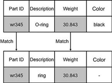
FIGURE 12.3 Deterministic record linkage.

Probabilistic algorithms provide a further level of configuration, and allow weights to be set for every attribute. Usually, there are two probabilities that need to be specified for an attribute. The first, m, is the probability that a common attribute agrees on a matching pair of records, and the second, u, is the probability that a common attribute agrees on an unmatched pair of records (nonmatching records agree simply by chance). For instance, gender usually has two possible values (female and male) that are uniformly distributed, and therefore there is a 50% chance that two records will have the same value for this attribute when they are not a match. These probabilities are used in the standard record linkage algorithms to give a final weight for each attribute, and then are summed to give an overall value that indicates whether the algorithm considers the two records to be a match or not.

In many cases, for a particular attribute, two records may have very similar values that are not exactly the same. Observe the “Description” field values in Figure 12.3 (O-ring and ring) that differ only by two characters. This type of difference is very common in all areas; names of people, addresses, and customer reference numbers may all contain small typographic errors that mean they do not match exactly. Approximate string matching (also known in some instances as fuzzy matching) can be used to address this problem, which effectively tolerates the various differences that can arise between values. Table 12.3 shows the typical examples that approximate string matching algorithms can handle. Using approximate string matching algorithms with record linkage algorithms is therefore very common and can lead to a more reliable record matching solution. Standard MDM solutions already contain these algorithms and they often provide intuitive and convenient ways of configuring the parameters to suit various cases.

Table 12.3

String Differences

To assist with approximate string matching, lexical analysis can first be applied to the data to help standardize the values. The difference is that with lexical analysis, the values are actually changed before the matching algorithm runs, whereas relying on approximate string matching means that the values do not actually change. The algorithm can tolerate the differences during its execution.

Semantic profiling

Semantic profiling is used to check predefined business rules that apply to a data set. There may be no explicit reference to the business rule within the data model, and only the users of the data set know what the rule is. Evidence of the rule may only exist in the data itself. An example business rule between two columns could be:

If “location” = 1, 2, 3, or 4, then “warehouse” = W1

If “location” = 5 or 6, then “warehouse” = W2

The “warehouse” field may be calculated automatically by the software application. However, if the data in the database is moved to another database that does not automatically calculate this rule, then violations of the rule may exist and the data would be inaccurate. Semantic profiling can, therefore, be used to detect violations of rules within the data by inspecting each instance of data and flagging values that do not adhere to the rule.

Summary

Each of the methods described in this section are powerful methods of automating the detection of information quality problems in large data sets. The methods are typical of what can be found within data profiling software tools. Information quality professionals use these software tools to support the analysis of the data, interpret the results, and report the information quality problems in a way that is meaningful to business managers.

Besides supporting professionals who provide information quality–related services for organizations, these types of methods can also be attached to information systems and applied continuously to detect reoccurring information quality problems. Many vendors provide “bolt on” data quality software that uses these types of methods to detect and also correct the problems before the data is entered into the relevant information system. The correction of the problems is often referred to as data cleaning, which is the process of modifying the actual data to correct problems. However, before jumping in and correcting each problem as it is found, the TIRM process suggests that first you need to assess the overall risk posed by the problems so that improvement of the information can be focused on the most critical areas.

InfoRAS: A risk analysis tool covering stage B of TIRM

While there are tools that can be used to perform some of the TIRM steps, one single tool has been developed by the authors to support all of the steps within stage B of TIRM process. The aim of stage B is to assess the information risks in the organization. The tool, referred to as the InfoRAS tool, provides features that can model and record the information captured for each step and also calculate the final risk score for each business process. This is an example of automation that supports humans in calculating the risk, rather than fully automating stage B of TIRM. Figure 12.4 shows the different components of the TIRM model that were introduced in Chapter 5 and that can be modeled within InfoRAS, starting with the business process on the left and finishing with the impact on business objectives on the right. We now briefly revisit the TIRM model before explaining the functioning of the InfoRAS tool.

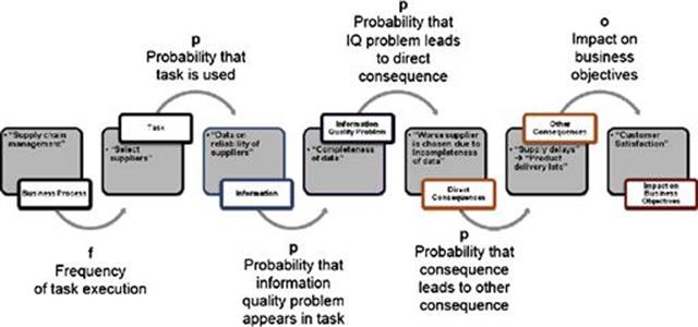
FIGURE 12.4 Components that can be modeled by the InfoRAS risk tool.

Each business process in the TIRM model contains any number of tasks that are carried out as part of that business process. For example, in Figure 12.4 selecting suppliers is an example task that is part of the supply chain management business process. A task may require the use of a particular piece of information (or multiple sets), such as, continuing the example, data on the reliability of suppliers. Each piece of information may contain information quality problems, such as missing entries (completeness of the data), which result in direct consequences. In the example in Figure 12.4, the worst supplier could be chosen based on not having the complete list of the suppliers. A direct consequence can lead to one or more intermediate consequences, and these intermediate consequences can have further consequences and so forth. For example, a poorly chosen supplier could result in supply delays, leading to a delayed final delivery of the product, which, in turn, could result in customer dissatisfaction. This is an example of an impact on the business objectives, which is the final part in the model in Figure 12.4.

As explained in Chapter 5, there are also five different parameters in the TIRM model that specify the link between the components in the model:

1. The frequency of task execution, which is the number of times (e.g., per month) that the task is actually carried out.

2. The probability that the information with the quality problems is needed.

3. The likelihood that the information quality problem appears in the information that is needed for the task needs to be specified.

4. The likelihood that the problem leads to the direct consequence along with the likelihood that each consequence leads to other consequences.

5. The severity of the impact in the impact on business objectives component.

InfoRAS actually accommodates a more in-depth recording of parameters than those described in the previous section. This is illustrated in Figure 12.5, which shows the parameters associated with a task node. As noted before, for each process the frequency with which the task is executed is recorded; however, rather than specify a single frequency number, it is far wiser to record a range that is very likely to contain the frequency. This was confirmed in the trials of the TIRM process in organizations, which found that it is often difficult to ascribe a single frequency number to a task with confidence, and it is easier to specify a range where the frequency resides. InfoRAS, therefore, allows the user to enter the lower bound, mode, and upper bound of the frequency with which the task is executed. The trials also found that in some cases the experts providing the estimates are very confident that the range captures the actual frequency, but in other cases they were found to be less confident. InfoRAS captures this uncertainty and allows the user to record the confidence, shown as the last parameter in Figure 12.5.

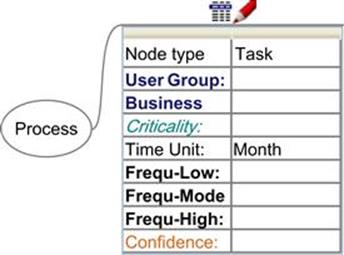
FIGURE 12.5 The process node and parameters for the task node in InfoRAS.

Specifying the range is not just applicable to the frequency that the tasks are executed in the process, but for every subsequent probability, as shown in Figure 12.4. InfoRAS allows the user to specify the range for every component. For example, in InfoRAS, each component contains the lower bound (%-Low), mode (%-Mode), upper bound (%-High), and confidence parameters, and these can be seen in Figure 12.6 for the information and information quality problem nodes. In some cases, an exact frequency may be known, in which case the same value can be entered in the lower bound, mode, and upper bound fields of InfoRAS. The final calculation performed by InfoRAS uses each of these values, with the confidence to calculate the overall risks to the business posed by the information quality problems. For the other parameters for the task, information, and information quality problem nodes, such as user group, and business process are informational only and can be used to provide further documentation about the different nodes. InfoRAS also provides a free text field that is associated with each node and can be used as needed; Figure 12.7 shows a screenshot of InfoRAS with the task1 node selected and the description field at the bottom. In this field, it is advisable to specify links to other documents, such as:

Process models that can help define the scope of the process and tasks.

The names of the databases or documents containing the information that is represented by the information node.

Information quality problem assessment documentation that is associated with the information quality problem nodes.

Detailed information about the risk controls that are already in place for the consequences.

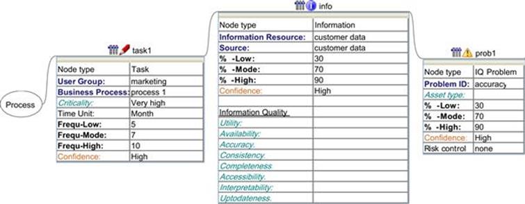
FIGURE 12.6 The parameters for the task, information, and information quality problem nodes in the InfoRAS tool.

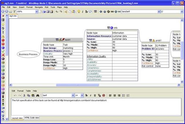
FIGURE 12.7 Screenshot of InfoRAS with notes.

Of these parameters, the time unit in the task node and the unit in the business impact node are very important, because when the final risk is calculated, it needs to be interpreted as, for example, pounds per month. The time unit in the task node is used to record whether it is per month and so forth, and the unit in the business impact is used to record the relevant currency. Note that this may not always need to be a currency: in some cases it could be a rating for health and safety or a measure of availability of a service.

The modeling of the consequences and the business impact using InfoRAS is shown in Figure 12.8. As noted before, any number of consequences can be recorded before reaching a business impact, and in the example in Figure 12.8, two consequences (c1 and c2) and their direct consequence (dc1) have been recorded. Note that this is the first version of the InfoRAS tool and therefore some functionality is yet to be included.

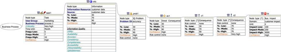
FIGURE 12.8 The direct consequence, other consequences, and business impact nodes in InfoRAS.

For simplicity, the example model of consequences and business impacts discussed previously was linear. InfoRAS, however, is capable of representing more complex relationships and can handle multiple tasks for a business process, multiple information resources for each task, and so on. Figure 12.9 shows a typical model that can be created with the tool, which contains two direct consequences that may result from a problem, three consequences, and three different business impacts (two are related to the impact on the customer and one to operational efficiency). As shown in Figure 12.9, InfoRAS presents this model in a clear and concise way, which enables analysts to clearly visualize the different impacts and chain of consequences.

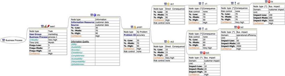
FIGURE 12.9 A more complicated example of the structures that can be modeled by InfoRAS.

One of the main advantages of InfoRAS is that it is able to calculate the total risks regardless of the complexity of the model and present aggregated results at each stage. Figure 12.10 shows the calculation for the example risk model in Figure 12.9, and the risk per annum is shown for each business impact node. For example, for bi1 the total risk is ≤30,632, for bi2 the total risk is ≤4243, and for bi3 the total risk is ≤105 per annum. The aggregated risk given by prob1 is the sum of each business impact that is related to this problem (in this case, ≤34980). There is only one problem and one task in this example, and so the overall risk to the business process is the same as for prob1. At the business process node, the results give a breakdown of the aggregated risk values for the IQ problem, data type, and business impact. When there are many IQ problems, information sets, and business impacts, having the results aggregated in this way is useful to help identify particular “pain points” within the business process that have a large effect on the overall risk.

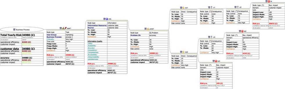
FIGURE 12.10 Risk total calculations with different levels of aggregation.

Software tools for detecting and treating information risks

In this section we discuss some of the example data risks that we found were common to many organizations, and show how existing software tools and techniques for managing information can be applied to automatically detect and mitigate the problems.

Example risk 1: Engineering Asset Management

Many organizations need to keep records about the locations and state of their physical assets. These may be trains, aircraft, underground water or gas pipes, electricity supply cables, and so on. Immediately, this does not sound like a very difficult task until you realize that some companies need to manage millions of physically distributed assets, of differing types that may be static or moving, cannot be easily taken offline for maintenance, and contain many dependent subcomponents. The asset management division in one organization we studied needs to maintain all of their assets in the most optimal way possible by saving time, resources, and costs. They carry out inspections of their assets, which are distributed throughout a large geographic area, before deciding whether or not to replace, repair, or refurbish an asset. These inspections take time, resources, and have an associated cost, and additionally, need to be optimized. These processes clearly rely on having good-quality information about the assets. Information about the assets includes details such as asset type, current and previous locations, current physical state, dates of previous (and predicted dates for) inspections and maintenance, and the subcomponents that may require maintenance. With poor-quality information about the assets, engineers struggle to keep track of what assets they have, which ones need maintaining, and which ones need replacing.

This information is stored in a combination of asset management systems, but the main system for location information is the geographic information system (GIS). The problem with the location information is that some asset locations are recorded in the system and the asset is not physically at that location. Other times, the asset information is not recorded in the system, but does actually exist in reality. This happens because there are limited procedures in place to help keep the actual state of the asset and the information about the asset in synchronization. For example, an asset may be moved physically from one place to another, but the records about this asset are not properly updated. The impact is that inspectors go out to the wrong locations expecting to find an asset (sometimes traveling long distances, costing time and fuel) only to find that it is not where it is expected to be. It is very costly, therefore, to find missing assets! Clearly this does not just affect inspections, but maintenance of the assets is not optimized, and some assets are not maintained at all because the GIS does not record their existence. In the cases of critically important assets, not properly maintaining the asset could cause it to fail and incur serious risks to the business.

With millions of assets to inspect and maintain and the current poor-quality data in the system, the question is what could the company do to address this and move toward being able to develop optimal inspection/maintenance strategies?

There are two approaches that can be taken to address this: either to leave the information as is and use risk controls to ensure that decision making does not result in a negative impact to the business, or attempt to improve the information.

The first approach aims to ensure that subsequent analysis and decisions are taken with suitable risk controls, based on the expected level of quality of the data needed to make the decision. This is appropriate if the information only supports the decision. However, if the information is used as a direct input to the decision, and it cannot sensibly be made without it, then there is no option but to attempt to improve the information.

When seeking to improve the information there are two parts to be considered: what to do to ensure that new information entering the GIS system is correct, and what to do to correct the existing poor-quality information.

ACTION TIP

When considering an automated solution to solve a data problem, consider both how to address the problems with the existing data, as well as how to address problems that could occur with new data that will be entered into the systems in the future.

Addressing the problem for new data entering the system

The current process, where engineers record their actions on paper and then enter the details into the GIS system later, is fraught with problems. Engineers forget to update the GIS system from the paper records, and it is also easy to misinterpret the paper notes if someone else is entering the data.

With the widespread use of handheld electronic devices, such as mobile phones and tablets, that are able to connect wirelessly to the Internet and therefore to the organizations backend systems, there are many possibilities to improve the quality of data capture. This data capture can now be done in real time (e.g., when the engineer has just finished an inspection or repair of an asset), increasing the chances of correctly capturing what has been done. In this case, entering the data gets closer to being part of the actual maintenance job, and is therefore less likely to be neglected.

Organizations are beginning to develop their own applications on mobile devices with bespoke user interfaces, which allow field workers to capture critical data in the easiest way possible while also supporting real-time validation checks. Being able to validate data in real time is a tremendous advantage because it can provide immediate feedback on the quality of the data and at the time when the engineer is observing the real entity that the data is describing. Obvious mistakes can be caught immediately and prevented from being entered into the backend system.

Improving the existing information

For improving the existing information, the obvious approach is that the organization could send out a team of people to check every asset and then perform a cross-check of this against the information in the GIS. Correctly, you may observe that this sounds rather resource and time intensive. In fact, because in many organizations of this type there are hundreds of thousands, if not millions, of assets that need to be cross-checked, the whole idea is just not practical. Some level of automation is required. How can the information be corrected without having to go and inspect every single asset?

If some of the information in the system (and other related systems) is known to be correct (e.g.,, due to recent asset inspections), this can be used to infer properties about the incorrect information based on knowing some of the rules about the assets. For example, if you know that if asset A exists, then so must asset B, and asset B is not in the GIS, then this implies that asset B is missing from the GIS. Note that if, to correct the data, asset B is entered into the system, then it is important to accompany this with metadata describing that inference was used to determine the existence of this asset.

ACTION TIP

Use the information in the systems that is known to be correct to infer properties about the other information to validate its accuracy and determine what the correct values are most likely to be. Moreover, update the metadata to describe when any inferences have been made when correcting the data.

In many cases, there may not be many rules or known-to-be-correct information in the system, but correcting all the information possible using this approach helps reduce the number of necessary physical inspections. This could drastically reduce the time and cost associated with improving the information.

ATTENTION

Do not expect to be able to correct all the data with inferred values because there may be many cases where there is no reliable (or authoritative) data to be used as a basis for inference. However, just validating and improving the data that is possible within this approach could prioritize what physical checks are required, as well as drastically reduce the need for these physical checks.

To automatically discover rules in data, data mining tools can be used. The following sections describe the different data mining methods that can be used to assist with automating the detection and correction of the data errors in the GIS while minimizing the need to physically cross-check the assets.

Association rule mining

Association rule mining can help to automatically discover regular patterns, associations, and correlations in the data. It is an ideal method to use to discover hidden rules in the asset data. In the asset management example, it could be used to discover the rules between different assets and their properties so that, for example, when there are assets missing in the GIS, it could be possible to infer what they might be.

Association rule mining can uncover what items frequently occur together and is often used in market-basket analysis, which is used by retailers to determine what items customers frequently purchase together. If dependencies exist between assets, such as asset A is always replaced with asset B (asset B may be a subcomponent or supporting device), then association rule mining can help identify these rules. The method does not operate only on simple examples like this, but can be used in general to find groups of assets that frequently “occur” (are replaced, maintained, disposed of, etc.) together, thus giving an indication of what you would expect to find in the GIS.

The analysis of what items frequently occur together is supported by two measures, and these give an indication of whether a pattern is interesting and should be investigated further. Considering a database that contains information about asset replacements, one may perform the analysis on this to determine what asset groups are usually replaced together and therefore what assets should exist in the group. Any missing assets in the system can be detected by requesting the assets at each physical site from the GIS and comparing this list to the list of assets in the group. Two measures that support this analysis to help determine the asset groups are confidence and support. A confidence value, for example, of 70%, indicates that when asset A is replaced there is a 70% chance that asset B will also be replaced. The support measure shows the percentage of transactions in the database that support this statement. For example, a support value of 20% means that of all the transactions in the database, 20% of them showed assets A and B being replaced together. Usually, thresholds are set so that only the most significant patterns are shown, rather than all patterns with low confidence and support values.

Maintained assets may not always appear as part of a single maintenance action, in which case the preceding method would not be able to identify patterns among the assets. To assist with this, within association rule mining there is another method that analyzes patterns that occur within a time sequence. If the maintenance actions each appear as a record in a database (transactional data), then sequential analysis can be applied to determine what records commonly occur close together. If the maintenance records indicate that it is common for the engineer to repair asset A, B, and then C within a short time span, then assets A, B, and C should be recorded in the GIS as appearing in relatively close proximal physical locations.

Semantic profiling

The data quality profiling method of semantic profiling (described previously) is a useful technique to apply to check the validity of any rules discovered by association rule mining. Rules can be encoded and then the profiler will traverse the data and record any violations of the rule.

As an example, association rule mining may have discovered the rule that water-pumping stations are often needed by canal locks. Semantic profiling could be used to check all cases when a pumping station does not exist near a lock, and it could flag these cases for further inspection. In this GIS, this requires checking the type of asset (e.g., water-pumping station or lock) and possibly its physical location (usually via latitude, longitude, and elevation coordinates). If for a particular water-pumping station there is no lock within say a half mile, then this would be something to investigate.

Furthermore, the simplest cases arise when there is a reference to an asset in one system, and the asset does not exist in the other. For example, semantic profiling could be used to identify missing references between the transactional maintenance records and the master data GIS records. If there is a maintenance record about a water pipe inspection, then the associated master data about this water pipe should exist; if not, then clearly there is a missing record.

Summary and discussion

Numerous organizations need to ensure that they properly maintain their business assets, whether they relate to managing facilities or the core engineering assets of the organization. For some organizations, such as utilities, transport, and engineering firms, this is a core part of the business. Errors in the data about the assets can easily result in serious risks to the business, as poor decision making is likely to result from erroneous data. The sheer scale of the data within many asset management–related systems makes automation a necessity for helping to improve the data. The automation may support the data gathering process, such as with mobile devices with instant data validation, or could support intelligent processing of the data to help reduce the time needed for physical validation of the data against the real-life situation.

Example risk 2: Managing spares and consumables

One information risk that we encountered was within the managing spares and consumables business process of a manufacturing organization. This organization needs to order parts that are used as material for their manufacturing processes. The organization strives to procure quality parts at the most competitive price from various suppliers. In some cases, supplier relationships and contracts are in place and in other cases procurement agents find other suppliers on an ad-hoc basis. The recording of their material consumption is critical for the organization to optimize the procurement of parts for their manufacturing, as well as ensuring that inventory levels are manageable. If perishable parts are ordered and not used within a certain time, then they need to be disposed of. This incurs significant costs for purchasing the part, storage of the part, and part disposal. Even nonperishable parts if they are not used within a reasonable length of time can degrade (as well as fall outside their warranty period) and take up valuable warehousing space. Conversely, if there are no parts available at the time the manufacturing process needs them, the manufacturing cannot continue. It is, therefore, imperative that the ordering of parts is optimized to keep the manufacturing processes operational while ensuring that the warehouses are not overloaded and parts are not degrading beyond their useful life.

In this organization an ERP system was being used to hold information about materials consumption from the manufacturing process. However, users of this system were complaining that the information was often out of date, sometimes incorrect or incomplete, and often difficult to interpret because there was no unified terminology for materials. The main reason for this was that the data on consumption was being recorded manually on paper-based forms and then being manually entered into the ERP system.

The impact was that parts were being ordered unnecessarily as it was not transparent which exact spares and consumable materials the company needed to order. This resulted in between 10% and up to 1000% higher prices for parts. The estimated risk probability was 10–20% for parts and 30–40% for consumables. This information risk resulted in yearly estimated losses of $6 million on average per production site.

The various problems found in the consumption information can be divided into two groups, which necessitate two different solutions. First, the problems of out-of-date, incorrect, and incomplete information caused by poor manual data entry can be addressed by reducing the manual data entry and introducing automated solutions to capture what is really happening with parts consumption. Second, the problems of not being able to interpret the parts because there is no unified terminology for materials requires changes to the information system that stores and provides access to the data for its users.

Automated track and trace technologies

Rather than having humans sense when a part has been taken from the warehouse and has been used on the production line it is possible to introduce automated methods that can detect these events and record them in a database. Technologies such as radio-frequency identification (RFID) can be used in appropriate situations to track and trace parts to determine their actual locations. These work by installing a small tag on the part, which uniquely identifies the part, and then installing readers at various locations (e.g., at the entry to a warehouse). When the tag passes by (or is near to) the reader, then the reader can record this event and the result is stored in the database. In its simplest form, this event can record a timestamp for when the event occurred and the unique identifier of the part. With this simple level of detail of data and a small amount of inference, it is possible to determine the location of parts. For example, if we wish to determine which parts are currently stored in a warehouse and when a part is taken out of the warehouse, we could first tag each one of the parts before they enter the warehouse. Then we could install a reader at the entrance to the warehouse that would record the new part entering the warehouse; we would know that it is a new part because there would be no previous record of the part in the database. When the part is taken from the warehouse it would pass out of the entrance and be read by the reader, and in this case we would know that the part is being removed because the previous database entry about this part would have recorded it coming in. So by observing the entries in the database and correlating these with reads of the part by the reader, we can determine where the part is. Clearly, this is a very simple example, and often there needs to be a series of readers at various locations. For example, there may be more than one exit or entrance to the warehouse. The same principle can be applied to determine the location of the part near the manufacturing line to determine when it is in the queue to be used as material input into the manufacturing process. The level of detail of the location of the part depends on the number of readers installed and how accurate these readers are at capturing the parts’ presence.

A side benefit to using this sort of technology is that business intelligence (BI) questions can be answered that give the business further insight into how the operations can be improved. For example, it would be simple to calculate the time each individual part spends in the warehouse if you automatically record time in and time out (by subtracting the timestamps for the part-out and part-in events recoded by the reader). With detailed records of each part’s time in the warehouse, it would be possible to optimize the purchase of part warranties to reduce the costs associated with parts falling out of warranty, as well as have a better understanding of which parts can be bought in batches of a certain size. As well as BI questions, this automation technology can clearly assist the operational decisions that are incurring unnecessary additional costs to the organization, such as whether to procure more of a certain type of part immediately or not. Any ways of improving the operations identified by these activities could be used to inform the information risk treatment stage of the TIRM process. By identifying and focusing on ways to optimize operations, the organization is essentially removing unnecessary procedures that may cause information risks in the first instance. This can operate the other way around too: if certain information risks are identified with the TIRM process, then treating these risks at the operational level is one option, but the organization may want to take a more strategic approach to avoiding the information risk. The TIRM process could, therefore, be used as an indicator for what BI-related questions should be posed to help steer the organization around information risks that cannot be treated with operational risk treatments.

Master data management

Regarding the problem of not having an unified terminology for materials, MDM is a key information management technology that can help to solve the problem.

At a simple level, a database could contain a list of parts that are referred to in multiple different ways. This same problem was introduced when describing reference data previously, with differences occurring in the recording of a country. In this example, it is a part that could be recorded in the database in multiple ways. For instance, the descriptions of parts are often in free text fields that allow the users to enter any description they like, which can clearly lead to all sorts of differences. However, even the part numbers can differ: the manufacturing organization may have their internal part number for a particular part, and this is likely to be different from the vendor’s part number. When the manufacturer receives the part from the vendor, the goods-received note contains the vendor number for the part, and this needs to be correlated with any other numbers for the part, just to establish if it is the same part.

MDM is a solution to this problem and can help provide the users of the organization’s information system with a single, consistent view of parts. Inconsistencies between master data are a problem common to many organizations; MDM is often used in other applications such as CRM and SRM. MDM relies on effective data governance, which provides the rules that the organization must adhere to when managing their data. With the preceding example, data governance should define exactly what a part is (and how it can be uniquely identified) and state, for example, what particular part numbers the organization will use (i.e., manufacturer or vendor part number) in different cases. Without this supporting knowledge, a master data solution has no basis from which it can sensibly merge duplicate parts. MDM solutions may not only be software but could also be a set of procedures that an organization follows. The aim of MDM is to provide a single (often referred to as a golden) version of the data and deliver it to the enterprise (any business unit) while enabling users to update the data in a way that does not reintroduce inconsistencies or errors into the data.

The key ongoing functions of MDM that are needed to ensure that entities (e.g., parts, customers, etc.) are consistent are to:

Detect and merge, if necessary, any duplicate entities into a single record.

Standardize any properties of the entities so that they are shown to the users consistently.

Provide data movement and integration facilities (e.g., ETL).

Collect all instances of an entity from various databases and present them as a single, consolidated list to the users.

Provide transaction services that support the creation, reading, updating, and deleting of the entities.

A dedicated software solution to MDM alone is unlikely to be effective to provide these functions. Organizations should also establish an effective data governance program and treat MDM as a data quality improvement process. The software solutions can therefore support these activities as required. There are many MDM solutions available from various vendors and they typically provide ways to automate the preceding functions. The following sections describe these various functions from the perspective of how they can be automated.

Detect and merge records

MDM solutions include matching algorithms (described previously), which help to detect whether two records refer to the same entity. These algorithms could help to detect overlaps in parts in the ERP system of the manufacturing organization. Once these algorithms have detected possible matching records, it is necessary to merge them, and this is one of the key pieces of functionality within MDM solutions.

The problems arise when the data values in two different records are inconsistent and it is necessary to choose the correct data value for the new master record. Rules that govern what data is carried forward to the consolidated master record are called survivorship rules and these are part of the merge algorithms. Most of the time, records will be gathered from multiple systems and so the rules need to define exactly which data and which system are to be trusted to provide the best data. Some example rules include:

1. If the value exists in system A, then choose this value, rather than the value from system B.

2. If there is only one value available (the others are missing), then take this value.

As an example of applying survivorship rules, consider what happens when creating a consolidated master record from the data from the two systems in Figure 12.11. With the “Part ID” and “Weight” values, there is no problem because they are consistent, and so these values can be taken and placed directly in the consolidated master record. For the “Color” field it is also relatively straightforward because the value in system B is missing and so the value from system A is chosen (in accordance with rule 2 above). For the description field there are two inconsistent values and this is the hardest case to cater for. Rule 1 states that system A is the authoritative source of reference, and so this value is taken to be included in the consolidated record. You can see how successful matching relies on developing strong rules that cater for the different scenarios that may arise.

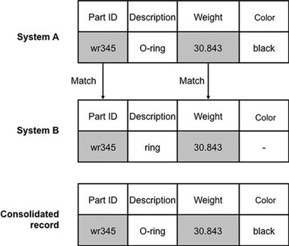
FIGURE 12.11 Survivorship example.

Standardization

In the manufacturing company example, the records of parts are spread between various databases and therefore the attribute names may not always be the same. For example, an attribute could be labeled “part_description” in one database and “desc.” in another. MDM solutions help to map between these values to indicate which attributes are semantically equivalent. Note that semantically equivalent attribute values may also be different between systems. For example, date fields may be formatted dd/mm/yyyy in one system and mm/dd/yyyy in another system, which means that the values also need to be mapped. This is referred to as standardization, and it is often performed during the transform step of an ETL process in many MDM solutions (see the previous section on lexical analysis). Even within the same database, there may be differences between the values for a particular attribute. A common example is with free text fields such as addresses or part descriptions that contain different punctuation marks and a mixture of short abbreviations and more fully expanded abbreviations, etc. In this case, standardization could help to present a common value format to all users or to map between these if different users require different formats. For example, standardization could help map between the semantically equivalent values “pneumatic actuator” and “act. pneumatic” by changing one to the other.

Usually before applying record linkage algorithms it is beneficial to standardize values making them more consistent. The record linkage algorithms, therefore, stand a better chance of matching similar values and do not have to rely on approximate string matching algorithms.

Architectures for MDM

Depending on the manufacturing organization’s individual information systems and how they are arranged, there are different possible MDM architectures that could be used to consolidate the parts records and provide transaction support to create, read, update, and delete the parts records.

There are a few different architectures for implementing MDM and it is common for organizations to develop these incrementally from the simplest to the most complex. In practice, while there are many possible ways of implementing these and small differences exist between the architectures, here we describe only the main architectures to give a general overview.

The registry implementation style is the simplest architecture and consists of a central hub system that holds the key data that relates to the master record (Figure 12.12). It only holds the data that is essential to determine the unique identity of the record and all other data related to the record are left in the source systems. This avoids unnecessary movement of data between the systems, and allows the users at the source systems to change most of the data without the hub even needing to know. The hub creates a globally unique identifier for each master data record and also holds a reference (cross-reference keys) to the associated record in the source systems. Updates are published to the hub system, using this reference, from each source system. Usually, there are no mechanisms that allow updating at the hub system and propagation of these updates to the source systems, and therefore, this type of architecture is useful when only needing to read the data from the hub. Being the simplest architecture, it is the easiest to implement.

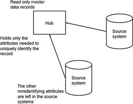
FIGURE 12.12 Registry MDM architecture.

For the manufacturing organization that needs to consolidate parts, this architecture is an ideal starting point to give the users read-only access to the consolidated parts. The transactional systems that track parts’ locations and usage can reference the master records for parts in the hub system as a single, reliable version of the truth. However, if the organization needs more than just read-only access to the master data, a new MDM architecture is required that builds on the registry architecture.

At the next level of complexity is the coexistence MDM architecture (Figure 12.13). In this architecture, the hub contains the full master record rather than only the uniquely identifying attributes (as in the registry architecture). Furthermore, not only are the updates from the source systems sent to the hub system, but also changes in the master record in the hub system are sent to subscribing source systems. This means that when an update to a record is made in the source system, the update is sent to the hub and then the update is sent out to all subscribing source systems. The difference in time between these updates means that the subscribing source systems may contain out-of-date information for the brief period before the synchronization is made.

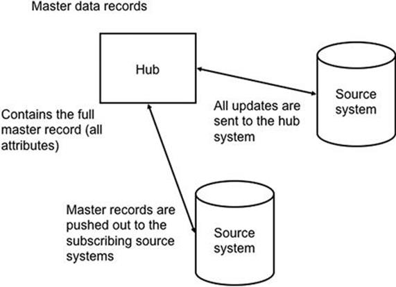
FIGURE 12.13 Coexistence MDM architecture.

The manufacturing company could use this architecture to distribute the parts records to the relevant source systems where they could be updated, and these updates would be reflected in the other subscribing systems.

The next level of complexity of MDM architecture is when all source systems are updated with the correct master data, referred to as the transactional architecture (Figure 12.14). This is an advanced and complex architecture because it extends the coexistence architecture by synchronizing data to all systems. This is done once the hub has integrated the relevant master data records from all the systems and resolved any inconsistencies.

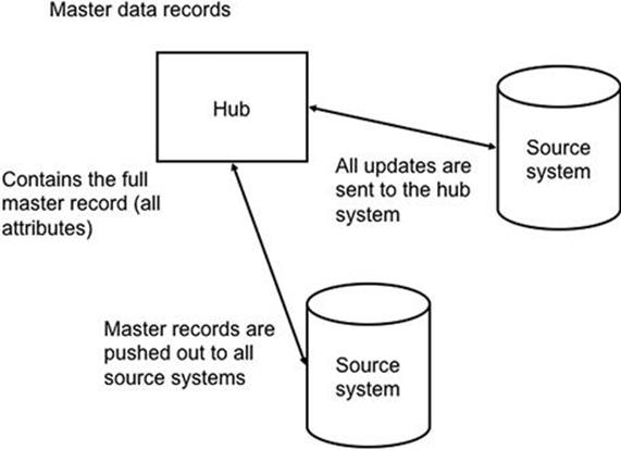
FIGURE 12.14 Transactional MDM architecture.

If the manufacturing organization implements this architecture, it can be sure that all parts records would be properly integrated and available at all systems. This is a complex architecture, and it means that additional effort needs to be expended to develop and maintain this system. The trade-off of whether to develop a system like this or stick with the simpler system should be based on the requirements of the organization, not the desire of IT or anyone else to have the “highest-level” architecture. For instance, if the manufacturing organization can fulfill its needs by using the registry architecture, then there is no need to develop this further.

IMPORTANT

The trade-off of whether to develop a system like this or stick with the simpler architecture should be based on the requirements of the organization, not the desire of IT or anyone else to have the “highest-level” architecture.

Note that the hub system referred to in all of the MDM architectures could be a new system or an adaption of one of the existing source systems. If there is one source system that contains the most authoritative list of master records and has good data integration capabilities, then this is a good candidate for the hub. The advantage is that it may already contain a lot of the master records, existing ETL operations to integrate the data, configured data cleansing capabilities, etc. The problem is that it would be necessary to ensure that the operational use of this system is not interrupted by making it the MDM hub. It would be easy to overlook the performance requirements of this system, which could be drastically affected if it turns into a transactional MDM architecture that requires the system to synchronize all updates to all source systems.

ACTION TIP

Consider whether to use an existing source system as the hub, but be wary about how this could negatively affect the operational use of this system.

Summary

With the use of track and trace technologies to automate the reliable capture of information and MDM solutions to ensure that differences in terminology can be automatically unified, there are many options to mitigate information risks with minimal human intervention. For many manufacturing organizations that need to keep track of the state of millions of consumable parts, these solutions are a necessity to address, otherwise they could lead to intractable problems that humans would quickly be overwhelmed by.

Conclusion

With the massive data sets used by today’s leading organizations, manual methods of correcting information quality problems and analyzing the data are no longer feasible nor wise to apply without support. Automated methods for processing this data are essential and they are becoming increasingly necessary to use for all data-related tasks. Not only are these methods necessary to deal with a significant volume of data that organizations collect daily, but also the speed at which it is necessary to make decisions places new constraints on how the data needs to be managed and analyzed.

Organizations now face customers who will take their business elsewhere if their needs and preferences are not immediately and properly addressed, or the information held about them is incorrect; it is no longer acceptable to take weeks to process data and obtain the results. In many of today’s applications, speed is of the highest importance, and reducing the time between the event, data analysis, and decision is paramount to commercial success. This relies heavily on keeping the information free of quality problems before being able to perform speedy analysis to obtain valid results.

Existing software tools and architectural approaches that can help automate information quality assessment and improvement provide the answer to cope with these speed and volume requirements. This chapter has introduced the different ways in which the stages of the TIRM process can be automated, as well as how automated information management technologies can be employed to address different problems in different data types.

Reference

1. Gao J, Koronios A, Kennett S, Scott H. Business Rule Discovery through Data Mining Methods. In: Amadi-Echendu JE, Brown K, Willett R, Mathew J, eds. Definitions, Concepts, and Scope of Engineering Asset Management. London: Springer; 2010;159–172.