Modern Cryptography: Applied Mathematics for Encryption and Informanion Security (2016)
PART I. Foundations
Chapter 4. Essential Number Theory and Discrete Math
In this chapter we will cover the following:
![]() Number systems
Number systems
![]() Prime numbers
Prime numbers
![]() Important number theory questions
Important number theory questions
![]() Modulus arithmetic
Modulus arithmetic
![]() Set theory
Set theory
![]() Logic
Logic
![]() Combinatorics
Combinatorics
Number theory is an exciting and broad area of mathematics. Although it is considered pure mathematics, there are applications for number theory in many fields. When you read Chapters 10 and 11 concerning asymmetric cryptography, you will find that all asymmetric algorithms are simply applications of some facet of number theory. This leads us to the question, What is number theory? Traditionally, number theory is defined as the study of positive, whole numbers. The study of prime numbers is a particularly important aspect of number theory. The Wolfram MathWorld web site (http://mathworld.wolfram.com/NumberTheory.html) describes number theory as follows:
Number theory is a vast and fascinating field of mathematics, sometimes called “higher arithmetic,” consisting of the study of the properties of whole numbers. Primes and prime factorization are especially important in number theory, as are a number of functions such as the divisor function, Riemann zeta function, and totient function.
If you already have a solid background in mathematics, you may be asking yourself how well this topic can be covered in a single chapter. After all, entire textbooks have been written on number theory and discrete mathematics. In fact, entire books have been written on just the subtopics, such as prime numbers, set theory, logic, combinatorics, and so on. How, then, can I hope to cover these topics in a single chapter? Allow me to set your mind at ease. First, keep in mind that the goal of this chapter is not to make you a mathematician (though I certainly would not be disappointed if after reading this you feel motivated to read more on mathematics, or perhaps take math courses at a university). Rather, the goal is to give you just enough number theory and information to help you understand the modern cryptographic algorithms we will be discussing in later chapters. For that reason, I have not included discussions on some items that would normally be covered when discussing number theory. The most obvious of these are proofs—you won’t see coverage of mathematical proofs in this chapter. There are countless books with very good coverage of proofs, including proofs of the very concepts and statements covered in this chapter. If you want to explore these mathematical proofs, you will have no trouble locating resources.
Note
Any one of these topics could certainly be explored in more depth, and I certainly encourage you to do so. For example if you are reading this book as part of a college course, I would hope it would motivate you to take a course in basic number theory or discrete math (if you haven’t done so already).
If you have a solid foundation in mathematics, this chapter provides a brief review. If you lack such a foundation, as famed author Douglas Adams once said, “Don’t panic.” You will be able to understand the material in this chapter. Furthermore, this chapter will be sufficient for you to continue your study of cryptography. If these topics are new to you, however, this chapter (along with Chapter 5) might be the most difficult chapters to understand. You might need to read the chapters more than once.
Note
I provide some study tips throughout this chapter, directing you to some external sources that offer more coverage of a particular topic, including books and web sites. Although all the web sites may not always be up and available, they are easy and free for you to access. If a URL is no longer available, I suggest you use your favorite search engine to search the topic.
Number Systems
The first step in examining number theory is to get a firm understanding of number systems. Although number theory is concerned with positive integers, some of the number sets include additional numbers. I mention all the number sets here, but the rest of the chapter will focus on those relevant to number theory. You probably had some exposure to number systems even in primary school.
Natural Numbers
Natural numbers, also called counting numbers, are so called because they come naturally—that is, this is how children first learn to think of numbers. If, for example, you look on your desk and count how many pencils you have, you can use natural numbers to accomplish this task. Many sources count only the positive integers: 1, 2, 3, 4, …, without including 0; other sources include 0. I do not normally include 0 as a natural number, though not everyone agrees with me. (For example, in The Nature and Growth of Modern Mathematics,1 author Edna Kramer argues that 0 should be included in the natural numbers. And despite this rather trivial difference of opinion with that esteemed author, I highly recommend that book as a journey through the history of mathematics.)
Note
The number 0 (zero) has an interesting history. Although to our modern minds, the concept of zero may seem obvious, it actually was a significant development in mathematics. Some indications point to the Babylonians, who may have had some concept of zero, but it is usually attributed to ninth-century India, where they were carrying out calculations using 0. If you reflect on that for a moment, you will realize that 0 as a number, rather than just a placeholder, was not known to ancient Egyptians and Greeks.
Negative Numbers
Eventually the natural numbers required expansion. Although negative numbers may seem perfectly reasonable to you and me, they were unknown in ancient times. Negative numbers first appeared in a book dating from the Han Dynasty in China (c. 260). In this book, the mathematician Liu Hui (c. 225–295) described basic rules for adding and subtracting negative numbers. In India, negative numbers first appeared in the fourth century and were routinely used to represent debts in financial matters by the seventh century.
The knowledge of negative numbers spread to Arab nations, and by at least the tenth century, Arab mathematicians where familiar with and using negative numbers. The famed book Kitab al-jabr wa l-muqabala, written by Al-Khwarizmi in about 825, from which we derive the word “algebra,” did not include any negative numbers at all (www.maa.org/publications/periodicals/convergence/mathematical-treasures-al-khwarizmis-algebra).
Rational and Irrational Numbers
Number systems have evolved in response to a need produced by some mathematical problem. Negative numbers, discussed in the preceding section, were developed in response to subtracting a larger integer from a smaller integer (3 – 5). A rational number is any number that can be expressed as the quotient of two integers. Like many early advances in mathematics, the formalization of rational numbers was driven by practical issues. Rational numbers were first noticed as the result of division (4/2 = 2, or 4 ÷ 2 = 2). (Note the two symbols most of us learn for division in modern primary and secondary school: ÷ and /. Now that is not a mathematically rigorous definition, nor is it meant to be.)
Eventually, the division of numbers led to results that could not be expressed as the quotient of two integers. The classic example comes from geometry. If you try to express the ratio of a circle’s circumference to its radius, for example, the result is an infinite number. It is often approximated as 3.14159, but the decimals continue on and no pattern repeats. If a real number cannot be expressed as the quotient of two integers, it is classified as an irrational number.
Real Numbers
Real numbers is the superset of all rational and irrational numbers. The set of real numbers is infinite. It is likely that all the numbers you encounter on a regular basis are real numbers, unless of course you work in certain fields of mathematics or physics. For quite a long time, real numbers were considered to be the only numbers that existed.
Imaginary Numbers
Imaginary numbers developed in response to a specific problem. As you undoubtedly know, if you multiple a negative with a negative you get a positive (–1 × –1 = 1). This becomes a problem, however, if you consider the square root of a negative number. Clearly, the square root of a positive number is also positive (√4 = 2, √1 = 1, and so on). But what is the square root of a negative 1? If you answer negative 1, that won’t work, because when you multiply two negative 1’s, the answer is a positive 1. This conundrum led to the development of imaginary numbers, which are defined as follows: i2 = –1 (or conversely √–1 = i). So the square root of any negative number can be expressed as some integer multiplied by i. A real number combined with an imaginary number is referred to as a complex number.
Note
As far back as the ancient Greeks, there seems to have been some concept of needing a number system to account for the square root of a negative number. But it wasn’t until 1572 that Rafael Bombelli first established formal rules for multiplying complex numbers.
Prime Numbers
Although the various numbers discussed in the preceding sections are interesting from a cryptography perspective, it is difficult to find a set of numbers that is more relevant than prime numbers. A prime number is a natural number greater than 1 that has no positive divisors other than itself and 1. (Note that the number 1 itself is not considered prime.) Many facts, conjectures, and theorems in number theory are related to prime numbers.
The fundamental theorem of arithmetic states that every positive integer can be written uniquely as the product of primes, where the prime factors are written in order of increasing size. Basically this means that any integer can be factored into its prime factors. This is probably a task you had to do in primary school, albeit with small integers. If you consider the fundamental theorem of arithmetic for just a moment, you can see that it is one (of many) indications of how important prime numbers are.
As first proven by Euclid (328–283 B.C.E.), an infinite number of primes exist. (Many other proofs of this have been constructed later by mathematicians such as Leonhard Euler [1707–1783] and Christian Goldbach [1690–1765], both of whom we will discuss later in this chapter.) How many primes are found in a given range of numbers is a more difficult problem. For example, there are four primes between 1 and 10 (2, 3, 5, 7). Then, between 11 and 20, there are four more (11, 13, 17, 19). However, there are only two primes between 30 and 40 (31, 37). In fact, as we progress through the positive integers, prime numbers become more sparse. (It has been determined that “the number of prime numbers less than x is approximately x/ln(x).” Consider the number 10, for example. The natural logarithm of 10 is approximately 2.302, 10/2.302 = 4.34, and we have already seen there are four primes between 1 and 10.)
Note
Euclid’s famous work, Elements, written around 300 B.C.E., contains a significant discussion of prime numbers, including theorems regarding there being an infinite number of primes.
Finding Prime Numbers
As you will discover later in this book, prime numbers are a key part of cryptographic algorithms such as RSA. How do you generate a prime number? An obvious first thought is to think of a number and then check to see if it has any factors. If it has no factors, it is prime. You can check by simply trying to divide that random number n by every number up to the square root of n. So, if I ask you if 67 is prime, you first try to divide it by 2, then by 3, then by 4, and so forth. In just a few steps, you will determine that 67 is a prime number. (That wasn’t so hard.) Using a computer, you could determine this much faster.
Unfortunately, for cryptographic algorithms such as RSA, we need much larger prime numbers. Modern RSA keys are a minimum of 2048 bits long and need two prime numbers to generate, and those prime numbers need to be very large. So simply generating a random number and checking it by hand is impossible to do and could take quite some time even with a computer. For this reason, there have been numerous attempts to formulate some algorithm that would consistently and efficiently generate prime numbers. Let’s look at just a few of those algorithms.
Mersenne Prime
French theologian Marin Mersenne (1588–1648) made significant contributions to acoustics and music theory as well as mathematics. He posited that the formula 2p – 1 would produce prime numbers. Investigation has shown that this formula will produce prime numbers for p = 2, 3, 5, 7, 13, 17, 19, 31, 67, 127, and 257, but not for many other numbers such as p = 4, 6, 8, 9, 10, 11, and so on. His conjecture resulted in a prime of the form 2p – 1 being named a Mersenne prime. By 1996, there were 34 known Mersenne primes, with the last eight discoveries made on supercomputers. Clearly, the formula can generate primes, but frequently it does not. Any number of the format 2p – 1 is considered a Mersenne number. It so happens that if p is a composite number, then so is 2p – 1. If p is a prime number, 2p – 1 might be prime. Mersenne originally thought all numbers of that form would be prime numbers.
Fermat Prime
Mathematician Pierre de Fermat (1601–1665) made many significant contributions to number theory. He also proposed a formula that he believed could be used to generate prime numbers:
2(2n) + 1
Several such numbers—particularly the first few powers of 2—are indeed prime, as you can see here:
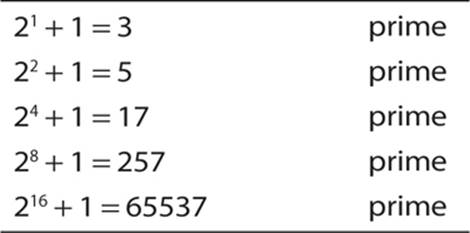
Unfortunately, as with Mersenne primes, not all Fermat numbers are prime.
Sieve of Eratosthenes
In some cases, the goal is not to generate a prime, but to find out if a known number is a prime. To determine whether a number is prime, we need some method(s) that are faster than simply trying to divide by every integer up to the square root of the integer in question. The Eratosthenes sieve is one such method. Eratosthenes (c. 276–195 B.C.E.) served as the librarian at the Library of Alexandria, and he was also quite the mathematician and astronomer. He invented a method for finding prime numbers that is still used today, called the sieve of Eratosthenes. It essentially filters out composite integers to leave only the prime numbers. The method is actually rather simple. To find all the prime numbers less than or equal to a given integer n by Eratosthenes’s method, you’d do the following:
1. Create a list of consecutive integers from 2 to n: (2, 3, 4, …, n).
2. Initially, let p equal 2, the first prime number.
3. Starting from p, count up in increments of p and mark each of these numbers greater than p itself in the list. These will be multiples of p: 2p, 3p, 4p, and so on. Note that some of them may have already been marked.
4. Find the first number greater than p in the list that is not marked. If there is no such number, stop. Otherwise, let p now equal this number (this is the next prime), and repeat from step 3.
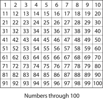
To illustrate, you can do this with a chart, such as the one shown next. For the purposes of demonstrating this concept we are concerning ourselves only with numbers through 100.
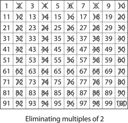
First, cross out the number 2, because it is prime, and then cross out all multiples of 2, since they are, by definition, composite numbers, as shown here:
Next, do the same thing with 3 (since it is also a prime number) and for all multiples of 3, as shown here:
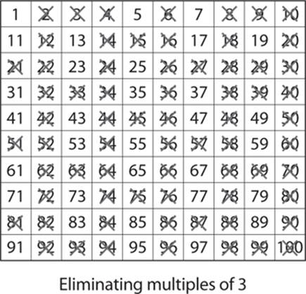
Notice that you’ve already crossed out many of those numbers, because they are also multiples of 2. You can skip 4, since it is a multiple of 2, and go straight to 5 and multiples of 5. Some of those (such as 15) are also multiples of 3 or multiples of 2 (such as 10, 20, and so on) and are already crossed out. You can skip 6, 8, and 9, since they are multiples of numbers that have already been used, and that leaves 7 and multiples of 7. Given that we are stopping at 100, you will find if you use 11 and multiples of 11, that will finish your application of the sieve of Eratosthenes. After you have crossed out multiples of 5, 7, and 11, only prime numbers remain. (Remember 1 is not prime.) You can see this here:
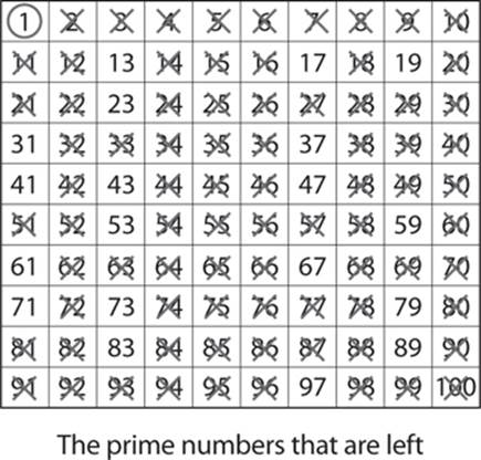
This can be a tedious process and is often implemented via a computer program. If you are going past 100, you just keep using the next prime number and multiples of it (13, 17, and so on).
Other Sieves
A number of more modern sieve systems have been developed, including the sieve of Atkin, developed in 2003 by Arthur O.L. Atkin and Daniel J. Bernstein, and the sieve of Sundaram, developed in the 1930s by mathematician S.P. Sundaram.
Like the sieve of Eratosthenes, the sieve of Sundaram operates by removing composite numbers, leaving behind only the prime numbers. It is relatively simple:
1. Start with a list of integers from 1 to some number n.
2. Remove all numbers of the form i + j + 2ij. The numbers i and j are both integers with 1 ≤ i <≤ j and i + j + 2ij ≤ n.
3. Double the remaining numbers and increment by 1 to create a list of the odd prime numbers below 2n + 2.
Lucas-Lehmer Test
The Lucas-Lehmer test is used to determine whether a given number n is a prime number. This deterministic test of primality works on Mersenne numbers—that means it is effective only for finding out if a given Mersenne number is prime. (Remember a Mersenne number is one of the form 2p – 1.) In 1856, French mathematician Édouard Lucas developed a primality test that he subsequently improved in 1878; then in the 1930s, American mathematician Derrick Lehmer provided a proof of the test.
Note
Throughout the study of cryptography you will encounter the terms “probabilistic” and “deterministic” in reference to primality tests, pseudo-random number generators, and other algorithms. The meanings of these two terms is fairly simple: A probabilistic algorithm has a probability of giving the desired result, and a deterministic algorithm will give the desired result. In reference to primality testing, a probabilistic test can tell you that a given number is probably prime, but a deterministic test will tell you that it is or is not definitely prime.
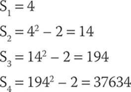
A Lucas-Lehmer number is part of a sequence of numbers in which each number is the previous number squared minus 2. So, for example, if you start with 4, you would get the sequence shown here:
The test is as follow:
For some p ≥ 3, which is itself a prime number, 2p – 1 is prime if and only if Sp–1 is divisible by 2p – 1. Example: 25 – 1 = 31; because S4 = 37634 and is divisible by 31, 31 must be a prime number.
Note
At this point, you may be tempted to question the veracity of a claim I made regarding the reliability of the Lucas-Lehmer test. As I stated at the beginning of this chapter, I will not be demonstrating mathematical proofs. You can spend some time with this test, using various values of S to see for yourself that it does, indeed, work. That is certainly not the same as working out a proof, but it could give you some level of comfort that the test really works.
Relatively Prime, or Co-prime, Numbers
The concept of prime numbers and how to generate them is critical to your study of cryptography. You should also be familiar with the concept of numbers that are relatively prime, often called co-prime numbers. The concept is actually pretty simple: Two numbers x and y are relatively prime (co-prime) if they have no common divisors other than 1. So, for example, the numbers 8 and 15 are co-prime. The factors of 8 are 1, 2, and 4, and the factors of 15 are 1, 3, and 5. Because these two numbers (8 and 15) have no common factors other than 1, they are relatively prime.
Lots of interesting facts are associated with co-prime numbers, many of which were discovered by Euler, who asked a few simple questions such as this: Given an integer n, how many numbers are co-prime to n? That number is called Euler’s totient, the Euler phi function, or simply the totient. The symbol for the totient of a number is shown here:
φ(n)
The term used for integers that are smaller than n and that have no common factors with n (other than 1) is totative. For example, 8 is a totative of 15. To check this easily yourself, you will see that 1, 2, 4, 7, 8, 11, 13, and 14 are all co-prime (or relatively prime) with 15. However, 3, 5, 6, 9, 10, and 12 all have common factors with 15.
Note
Euler introduced this function in 1763. There was no practical use for it until modern asymmetric cryptography. This is a great example of pure mathematics that is later found to have very important practical applications.
The next question Euler asked was this: What if a given integer, n, is a prime number? How many totatives will it have (that is, what is the totient of n)? Let’s consider a prime number—for example, 7. Given that 7 is prime, we know that none of the numbers smaller than 7 have any common factors with 7. So 2, 3, 4, 5, and 6 are all totatives of 7. And since 1 is a special case, it is also a totative of 7, so we find that six numbers are totatives of 7. It turns out that for any n that is prime, the Euler’s totient of n is n – 1. So if n = 13, then the totient of n is 12.
And then Euler asked yet another question about co-prime numbers: Assuming we have two prime numbers, m and n. We already know that the totient of each is m – 1 and n – 1, respectively. But what happens if we multiply the two numbers together? So m × n = k; what is the totient of k? You could simply test every number less than k and find the answer. That might work for small values of k, but it would be impractical for larger values. Euler discovered a nice shortcut: If you have two prime numbers (m and n) and multiply them to get k, the totient of k is the totient of m × the totient of n. Put another way, the totient of k is (m – 1)(n – 1).
Let’s look at an example. Assume we have two prime numbers, n = 3 and m = 5.
1. Multiply n × m: 3 × 5 = 15.
2. The totient of n is n – 1, or 2.
3. The totient of m is m – 1, or 4.
4. 2 × 4 = 8
5. The totient of k (15) is 8.
The totient, 15, is a small number so we can test it. The factors of 15 (other than 1) are 3 and 5, which means that 15 has common factors with any multiple of 3 or 5 smaller than 15: 3, 6, 9, 12 and 5, 10. So with what numbers does 15 not have common factors? 1, 2, 4, 7, 8, 11, 13, and 14. If you take a moment to count those, you will see that there are eight numbers. Of course, Euler relied on rigorous mathematical proofs, which we are foregoing in this chapter, but hopefully this example provides you with a comfort level regarding calculating totients.
Now all of this may sound rather obscure, or even unimportant. However, these facts are a very big part of the RSA algorithm that we will be examining in some depth in Chapter 10. In fact, when you first see the RSA algorithm, you will notice several elements discussed in this section.
Important Operations
Some mathematical operations are critical even to a basic understanding of modern cryptographic algorithms. Those of you with a solid foundation in mathematics should already be familiar with these operations, but in case you are not, I will briefly introduce you to them in this section.
Divisibility Theorems
You should be aware of some basics about divisibility that define some elementary facts regarding the divisibility of integers. The following are basic divisibility theorems that you will see applied in later chapters in specific cryptographic algorithms. I recommend that you commit them to memory before proceeding.
For integers a, b, and c, the following is true:
![]() If a | b and a | c, then a | (b + c). Example: 3 | 6 and 3 | 9, so 3 | 15. (Note that | means divides, so in this statement, if a divides b and a divides c, then a will divide b + c.)
If a | b and a | c, then a | (b + c). Example: 3 | 6 and 3 | 9, so 3 | 15. (Note that | means divides, so in this statement, if a divides b and a divides c, then a will divide b + c.)
![]() If a | b, then a | bc for all integers c. Example: 5 | 10, so 5 | 20, 5 | 30, 5 | 40, ….
If a | b, then a | bc for all integers c. Example: 5 | 10, so 5 | 20, 5 | 30, 5 | 40, ….
![]() If a | b and b | c, then a | c. Example: 4 | 8 and 8 | 24, so 4 | 24.
If a | b and b | c, then a | c. Example: 4 | 8 and 8 | 24, so 4 | 24.
Summation
You have probably seen the summation symbol, ∑, frequently. If not, you will see it later in this book. It is basically a way of adding a sequence of numbers to get their sum. It is more convenient to use the summation symbol than expressly write out the summation of a long series of values. Any intermediate result at any given point in the sequences is a partial sum (sometimes called a running total or prefix sum). The numbers that are to be added up are often called addends or sometimes summands. They can be any numbers, but in cryptography, we are most often interested insumming integers.
A basic example of summation is shown in Figure 4-1.
![]()
FIGURE 4-1 A summation
The figure states that we are dealing with some integer i. We begin with the value of i set to 1. Add up the i values from 1 until you reach 100. The letter to the right of the summation symbol is the variable we are dealing with. The number under the summation is the initial value of that variable. Finally, the number over the summation symbol (often denoted with an n) is the stopping point. You can manually add these numbers up, 1 + 2 + 3 + 4 … 100, if you wish; however, you can use a formula to compute this summation:
(n(n+1))/2
In our example, that is
(100(101))/2 = 5050
Note
The notation you see used in Figure 4-1 is often called the “capital Sigma notation,” because the ∑ is the Greek sigma symbol.
You can do a similar operation with multiplication using the pi symbol, ![]() . This symbol works exactly like the capital Sigma notation, except rather than adding up the series of values to arrive at a sum, you multiply the series of values to arrive at a product.
. This symbol works exactly like the capital Sigma notation, except rather than adding up the series of values to arrive at a sum, you multiply the series of values to arrive at a product.
Logarithms
Logarithms play a very important role in asymmetric cryptography. An entire class of asymmetric algorithms are based on what is called the discrete logarithm problem. Most readers encountered logarithms during secondary school.
The logarithm of a number is the exponent to which some fixed value (called the base) must be raised to produce that number. Let’s assume base 10, for example, and ask, what is the logarithm of 10,000? In other words, what number must 10 be raised to in order to produce the number 10,000? The answer is 4, as 104 = 10,000. Most people are quite comfortable with base 10, which is known as the common logarithm in mathematics. However, we can use any base. For example, suppose we want to know the logarithm of 16 in base 2, which we would write as log2(16). In other words, what power must 2 be raised to in order to get 16? The answer is 4, as 24 = 16.
Natural Logarithm
The natural logarithm, denoted as ln, is widely used in math and science. Natural logarithms use the irrational number e (approximately 2.718) as the base. The natural logarithm of some number x is usually written as ln x but can also be written as loge x. As with any logarithm, the natural log is what power e must be raised to in order to give some particular number.
The basic concept of the natural logarithm was developed by Grégoire de Saint-Vincent and Alphonse Antonio de Sarasa in the early 17th century. They were working on problems involving hyperbolic sectors.
Tip
If you are new to logarithms and/or natural logs, you may wish to consult two tutorials to learn more about these topics: “The Common and Natural Logarithms” at http://www.purplemath.com/modules/logs3.htm and “Demystifying the Natural Logarithm (ln)” athttp://betterexplained.com/articles/demystifying-the-natural-logarithm-ln/.
Discrete Logarithm
Now that you have a basic grasp of logarithms and even natural logs, we can turn our attention to discussing discrete logarithms. These play an important role in the algorithms we will explore in Chapters 10 and 11.
To understand discrete logarithms, keep in mind the definition of a logarithm: the number to which some base must be raised to get another number. Discrete logarithms ask this same question, but do so with regard to a finite group. Put more formally, a discrete logarithm is some integer k that solves the equation xk = y, where both x and y are elements of a finite group.
Computing a discrete logarithm is a very difficult problem, which is why discrete logarithms form the basis for some modern cryptographic algorithms. We will take up this topic again in Chapter 10 when we discuss specific algorithms and after we have discussed groups in Chapter 5. For now, note that a discrete logarithm is, essentially, a logarithm within some finite group.
Tip
The Kahn Academy web site provides a very nice introduction to discrete logarithms: https://www.khanacademy.org/computing/computer-science/cryptography/modern-crypt/v/discrete-logarithm-problem.
Modulus Operations
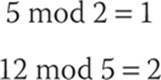
Modulus operations are important in cryptography, particularly in RSA. Let’s begin with the most simple explanation, and then delve into more details. To use the modulus operator, simply divide A by N and return the remainder. So, for example,
Note
I am not using the congruence symbol (≡) here because I am not discussing congruence. I am stating that if you divide 5 by 2, the remainder is 1, and if you divide 12 by 5, the remainder is 2. This is standard to computer programmers but might seem a bit odd to mathematicians. In many programming languages, the % symbol is used to perform the modulus operation.
This explains how to use the modulus operator, and in many cases this is as far as many programming textbooks go. But this still leaves the question of why we are doing this. Exactly what is a modulus? One way to think about modulus arithmetic is to imagine doing any integer math you might normally do, but bind your answers by some number. A classic example used in many textbooks is a clock, which includes numbers 1 through 12, so any arithmetic operation you do has to have an answer of 12 or less. If it is currently 4 o’clock and I ask you to meet me in 10 hours, simple math would say I am asking you to meet me at 14 o’clock. But that is not possible, because our clock is bounded by the number 12! Finding the answer is simple, though: use the mod operator with a modulus of 12 and look at the remainder:
14 mod 12 = 2
So I am actually asking you to meet me at 2 o’clock. (Whether that is A.M. or P.M. depends on the original 4 o’clock, but that is really irrelevant to understanding the concepts of modular arithmetic.) This is an example of how you might use modular arithmetic every day.
Note
Although the basic concept of modular arithmetic dates back to Euclid, who wrote about it in his book Elements, the modern approach to modular arithmetic was first published by Carl Friedrich Gauss in his book Disquisitiones Arithmeticae in 1801.
Congruence
Congruence in modulus operations is a very important topic and you will see it applied frequently in modern cryptographic algorithms. The symbol ≡ is used to denote congruence in mathematics.
Two numbers a and b are said to be “congruent modulo n” if
(a mod n) = (b mod n) → a ≡ b(mod n)
If two numbers are congruent modulo n, then the difference between a and b will be some multiple of n. To make this clearer, let’s return to the clock analogy, in which 14 and 2 are congruent modulo 12. It turns out that the difference between 14 and 2 is 12, a multiple of n (1 × 12). We also know that 14, or 1400 hours on the 24-hour clock, is 2 o’clock. So when we say that 14 and 2 are congruent modulo 12, we are stating that, at least in reference to modulo 12, 14 and 2 are the same. Here’s another example: 17 and 5 are congruent modulo 12. The difference between them is 12. Again using the 24-hour clock to test our conclusions, we find that 1700 hours is the same as 5 P.M.
You should be aware of some basic properties of congruence:
![]() a ≡ b (mod n) if n|(a – b)
a ≡ b (mod n) if n|(a – b)
![]() a ≡ b (mod n) implies b ≡ a (mod n)
a ≡ b (mod n) implies b ≡ a (mod n)
![]() a ≡ b (mod n) and b ≡ c (mod n) imply a ≡ c (mod n)
a ≡ b (mod n) and b ≡ c (mod n) imply a ≡ c (mod n)
Congruence Classes
A congruence class, or residue class, is a group of numbers that are all congruent for some given modulus.
Consider an example where the modulus is 5. What numbers are congruent modulo 5? Let’s begin with 7: 7 mod 5 ≡ 2. Next, we ask what other numbers’ mod 5 ≡ 2, and we arrive at an infinite series of numbers: 12, 17, 22, 27, 32 …. Notice that this works the other way as well (with integers smaller than the modulus, including negatives). We know that 7 mod 5 ≡ 2, but also 2 mod 5 ≡ 2 (that is, the nearest multiple of 5 would be 0; 0 × 5, thus 2 mod 5 ≡ 2). Make sure you fully understand why 2 mod 5 ≡ 2, then we can proceed to examine negative numbers. Our next multiple of 5 after 0, going backward, is –5 (5 × –1). So –3 mod 5 ≡ 2. We can now expand the elements of our congruence class to include –3, 0, 2, 7, 12, 17, 22, 27, 32, and so on.
You should also note that for any modulus n, there are n congruence classes. If you reflect on this for just a moment you should see that the modulus itself creates a boundary on the arithmetic done with that modulus, so it is impossible to have more congruence classes than the integer value of the modulus.
Modulus operations are very important to several asymmetric cryptography algorithms that we will be examining in Chapter 10. So make certain you are comfortable with these concepts before proceeding.
Tip
For more on modulus arithmetic, consult the Rutgers University tutorial “Modular Arithmetic” at www.math.rutgers.edu/~erowland/modulararithmetic.html, or TheMathsters YouTube video “Modular Arithmetic 1” at www.youtube.com/watch?v=SR3oLCYoh-I.
Famous Number Theorists and Their Contributions
When learning any new topic, you may often find it helpful to review a bit of its history. In some cases, this is best accomplished by examining some of the most important figures in that history. Number theory is replete with prominent names. In this section I have restricted myself to a brief biography of mathematicians whose contributions to number theory are most relevant to cryptography.
Fibonacci
Leonardo Bonacci (1170–1250), known as Fibonacci, was an Italian mathematician who made significant contributions to mathematics. He is most famous for the Fibonacci numbers, which represent an interesting sequence of numbers:
1, 1, 2, 3, 5, 8, 13, 21, …
The sequence is derived from adding the two previous numbers. To put it in a more mathematical format,
Fn = Fn–1 + Fn–2
So in our example, 2 is 1 + 1, 3 is 2 + 1, 5 is 3 + 2, 8 is 5 + 3, and so on.
The sequence continues infinitely. Fibonacci numbers were actually known earlier in India, but they were unknown in Europe until Fibonacci rediscovered them. He published this concept in his book Liber Abaci. Although this number series has many interesting applications, for our purposes, the most important is its use in pseudo-random number generators that we will be exploring in Chapter 12.
Fibonacci was the son of a wealthy merchant and was able to travel extensively. He spent time in the Mediterranean area studying under various Arab mathematicians. In his book Liber Abaci, he also introduced Arabic numerals, which are still widely used today.
Fermat
Pierre de Fermat (1601–1665) was trained as a lawyer and was an amateur mathematician, although he made significant contributions to mathematics. He worked with analytical geometry and probability but is best known for several theorems in number theory, which we will look at briefly.
Fermat’s little theorem states that if p is a prime number, then for any integer a, the number ap – a is an integer multiple of p. What does this mean? Let’s look at an example: Suppose a = 2 and p = 5. Then 25 = 32 and 32 – 2 is 30, which is indeed a multiple of p (5). This actually turns into a primality test. If you think p is a prime number, you can test it. If it is prime, then ap–a should be an integer multiple of p. If it is not, then p is not prime.
Let’s test this on some numbers we know are not prime. Use p = 9: 28 – 2 = 256 – 2 = 250, and 250 is not prime. This is an example of how various aspects of number theory, that might not at first appear to have practical applications, can indeed be applied to practical problems.
Note
This theorem is often stated in a format using modulus arithmetic. However, we have not yet discussed modulus arithmetic so I am avoiding that notation at this time.
Fermat first articulated this theorem in 1640, which he worded as follows:
p divides ap–1 – 1 whenever p is prime and a is co-prime to p
Fermat is perhaps best known for Fermat’s Last Theorem, sometimes called Fermat’s conjecture (which, incidentally, is no longer a conjecture). This theorem states that no three positive integers (x, y, z) can satisfy the equation xn + yn = cn for any n that is greater than 2. Put another way, if n > 2, then there is no integer to the n power that is the sum of two other integers to the n power. Fermat first proposed this in 1637, actually in handwritten notes in the margin of his copy of Arithmetica, an ancient Greek text written in about 250 C.E. by Diophantus of Alexandria. Fermat claimed to have a proof that would not fit in the margin, but it has never been found. However, his theorem was subsequently proven by Stanford University professor Andrew Wiles in 1994.
Euler
Swiss mathematician and physicist Leonhard Euler (1707–1783) is an important figure in the history of mathematics and number theory. Euler (pronounced oy-ler) is considered one of the best mathematicians of all time, and he is certainly the pinnacle of 18th-century mathematics.
Euler’s father was a pastor of a church. As a child, Euler and his family were friends with the Bernoulli family, including Johann Bernoulli, a prominent mathematician of the time. Euler’s contributions to mathematics are very broad. He worked in algebra, number theory, physics, and geometry. The number e you probably encountered in elementary calculus courses (approximately 2.7182), which is the base for the natural logarithm, is named after Euler, as is the Euler-Mascheroni constant.
Euler was responsible for the development of infinitesimal calculus and provided proof for Fermat’s little theorem, as well as inventing the totient function discussed earlier in this chapter. He also made significant contributions to graph theory. Graph theory is discussed later in this chapter in reference to discrete mathematics.
Goldbach
Christian Goldbach (1690–1765) was trained as a lawyer, but he is remembered primarily for his contributions to number theory. It is reported that he had discussions and interactions with a number of famous mathematicians, including Euler. Although he made other contributions to number theory, he is best remembered for Goldbach’s conjecture, which, at least as of this writing, is an unsolved mathematical problem. The conjecture can be worded quite simply:
Every integer greater than 2 can be expressed as the sum of two prime numbers. For small numbers, this is easy to verify (though the number 3 immediately poses a problem as mathematicians don’t generally consider 1 to be prime):
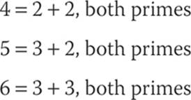
Although this is true for very large numbers and no exception has been found, it has not been mathematically proven.
Discrete Mathematics
As you learned in the discussion of number theory, some numbers are continuous. For example, real numbers are continuous—that is, there is no clear demarcation point. Consider 2.1 and 2.2 for example, which can be further divided into 2.11, 2.12, 2.13...2.2. And even 2.11 and 2.11 can be further divided into 2.111, 2.112, 2.113...2.12. This process can continue infinitely. Calculus deals with continuous mathematics. One of the most basic operations in calculus, the limit, is a good example of this.
Discrete mathematics, however, is concerned with mathematical constructs that have clearly defined (that is, discrete) boundaries. You can probably already surmise that integers are a major part of discrete mathematics, but so are graphs and sets.
Set Theory
Set theory is an important part of discrete mathematics. A set is a collection of objects called the members or elements of that set. If we have a set, we say that some objects belong (or do not belong) to this set, and are (or are not) in the set. We say also that sets consist of their elements.
As with much of mathematics, terminology and notation is critical. So let’s begin our study in a similar fashion, building from simple to more complex concepts. The simplest way I can think of is defining an element of a set: We say that x is a member of set A. This can be denoted as
![]()
Sets are often listed in brackets. For example the set of all odd integers < 10 would be shown as follows:
A = {1, 3, 5, 7, 9}
A member of that set would be denoted as follows:
![]()
Negation can be symbolized by a line through a symbol:
![]()
In this example, 2 is not an element of set A.
If a set is not ending, you can denote that with ellipses. For example, the set of all odd numbers (not just those less than 10) can be denoted like this:
A = {1, 3, 5, 7, 9, 11, …}
You can also denote a set using an equation or formula that defines membership in that set.
Sets can be related to each other, and the most common relationships are briefly described here:
![]() Union With two sets A and B, elements that are members of A, B, or both represent the union of A and B, symbolized as A ∪ B.
Union With two sets A and B, elements that are members of A, B, or both represent the union of A and B, symbolized as A ∪ B.
![]() Intersection With two sets A and B, elements that are in both A and B are the intersection of sets A and B, symbolized as A ∩ B. If the intersection of set A and B is empty (that is, the two sets have no elements in common), the two sets are said to be disjoint, or mutually exclusive.
Intersection With two sets A and B, elements that are in both A and B are the intersection of sets A and B, symbolized as A ∩ B. If the intersection of set A and B is empty (that is, the two sets have no elements in common), the two sets are said to be disjoint, or mutually exclusive.
![]() Difference With two sets A and B, elements that are in one set but not both are the difference between A and B, symbolized as A \ B.
Difference With two sets A and B, elements that are in one set but not both are the difference between A and B, symbolized as A \ B.
![]() Complement With two sets A and B, set B is the complement of set A if B has no elements that are also in A, symbolized as B = Ac.
Complement With two sets A and B, set B is the complement of set A if B has no elements that are also in A, symbolized as B = Ac.
![]() Double complement The complement of a set’s complement is that set itself. In other words, the complement of Ac is A. That may seem odd at first read, but reflect on the definition of the complement of a set for just a moment. The complement of a set has no elements in that set. So it stands to reason that to be the complement of the complement of a set, you would have to have all elements within the set.
Double complement The complement of a set’s complement is that set itself. In other words, the complement of Ac is A. That may seem odd at first read, but reflect on the definition of the complement of a set for just a moment. The complement of a set has no elements in that set. So it stands to reason that to be the complement of the complement of a set, you would have to have all elements within the set.
These are basic set relationships. Now a few facts about sets:
![]() Order is irrelevant {1, 2, 3} is the same as {3, 2, 1} or {3, 1, 2} or {2, 1, 3}.
Order is irrelevant {1, 2, 3} is the same as {3, 2, 1} or {3, 1, 2} or {2, 1, 3}.
![]() Subsets Set A could be a subset of set B. For example, if set A is the set of all odd numbers < 10 and set B is the set of all odd numbers < 100, then set A is a subset of set B. This is symbolized as A
Subsets Set A could be a subset of set B. For example, if set A is the set of all odd numbers < 10 and set B is the set of all odd numbers < 100, then set A is a subset of set B. This is symbolized as A ![]() B.
B.
![]() Power set Sets may have subsets. For example, set A is all integers < 10, and set B is a subset of A with all prime numbers < 10. Set C is a subset of A with all odd numbers < 10. Set D is a subset of A with all even numbers < 10. We could continue this exercise making arbitrary subsets such as E = {4, 7}, F {1, 2, 3}, and so on. The set of all subsets of a given set is called the power set for that set.
Power set Sets may have subsets. For example, set A is all integers < 10, and set B is a subset of A with all prime numbers < 10. Set C is a subset of A with all odd numbers < 10. Set D is a subset of A with all even numbers < 10. We could continue this exercise making arbitrary subsets such as E = {4, 7}, F {1, 2, 3}, and so on. The set of all subsets of a given set is called the power set for that set.
Sets also have properties that govern the interaction between sets. The most important of these properties are listed here:
![]() Commutative Law The intersection of set A with set B is equal to the intersection of set B with set A. The same is true for unions. Put another way, when considering intersections and unions of sets, the order in which the sets are presented is irrelevant. This is symbolized as shown here:
Commutative Law The intersection of set A with set B is equal to the intersection of set B with set A. The same is true for unions. Put another way, when considering intersections and unions of sets, the order in which the sets are presented is irrelevant. This is symbolized as shown here:
(a) A ∩ B = B ∩ A
(b) A ∪ B = B ∪ A
![]() Associative Law If you have three sets and the relationships among the three are all unions or all intersections, then the order does not matter. This is symbolized as shown here:
Associative Law If you have three sets and the relationships among the three are all unions or all intersections, then the order does not matter. This is symbolized as shown here:
(a) (A ∩ B) ∩ C = A ∩ (B ∩ C)
(b) (A ∪ B) ∪ C = A ∪ (B ∪ C)
![]() Distributive Law This law is a bit different from the Associative Law, and order does not matter. The union of set A with the intersection of B and C is the same as the union of A and B intersected with the union of A and C. This is symbolized as shown here:
Distributive Law This law is a bit different from the Associative Law, and order does not matter. The union of set A with the intersection of B and C is the same as the union of A and B intersected with the union of A and C. This is symbolized as shown here:
(a) A ∪ (B ∩ C) = (A ∪ B) ∩ (A ∪ C)
(b) A ∩ (B ∪ C) = (A ∩ B) ∪ (A ∩ C)
![]() De Morgan’s Laws These laws govern issues with unions and intersections and the complements thereof. These are more complex than the previously discussed laws. Essentially the complement of the intersection of set A and set B is the union of the complement of A and the complement of B. The symbolism of De Morgan’s Laws are shown here:
De Morgan’s Laws These laws govern issues with unions and intersections and the complements thereof. These are more complex than the previously discussed laws. Essentially the complement of the intersection of set A and set B is the union of the complement of A and the complement of B. The symbolism of De Morgan’s Laws are shown here:
(a) (A ∩ B)c = Ac ∪ Bc
(b) (A ∪ B)c = Ac ∩ Bc
These are the basic elements of set theory. You should be familiar with them before proceeding.
Logic
Logic is an important topic in mathematics as well as in science and philosophy. In discrete mathematics, logic is a clearly defined set of rules for establishing (or refuting) the truth of a given statement. Although I won’t be delving into mathematical proofs in this book, should you choose to continue your study of cryptography, at some point you will need to examine proofs. The formal rules of logic are the first steps in understanding mathematical proofs.
Logic is a formal language for deducing knowledge from a small number of explicitly stated premises (or hypotheses, axioms, or facts). Some of the rules of logic we will examine in this section might seem odd or counterintuitive. Remember that logic is about the structure of the argument, not so much the content.
Before we begin, I will define a few basic terms:
![]() Axiom An axiom (or premise or postulate) is something assumed to be true. Essentially, you have to start from somewhere. Now you could, like the philosopher Descartes, begin with, “I think therefore I am” (Cogito ergo sum), but that would not be practical for most mathematical purposes. So we begin with some axiom that is true by definition. For example, any integer that is evenly divisible only by itself and 1 is considered to be prime.
Axiom An axiom (or premise or postulate) is something assumed to be true. Essentially, you have to start from somewhere. Now you could, like the philosopher Descartes, begin with, “I think therefore I am” (Cogito ergo sum), but that would not be practical for most mathematical purposes. So we begin with some axiom that is true by definition. For example, any integer that is evenly divisible only by itself and 1 is considered to be prime.
![]() Statement This is a simple declaration that states something is true. For example, “3 is a prime number” is a statement, and so is “16 is 3 cubed”—it is an incorrect statement, but it is a statement nonetheless.
Statement This is a simple declaration that states something is true. For example, “3 is a prime number” is a statement, and so is “16 is 3 cubed”—it is an incorrect statement, but it is a statement nonetheless.
![]() Argument An argument is a sequence of statements. Some of these statements, the premises, are assumed to be true and serve as a basis for accepting another statement of the argument, called the conclusion.
Argument An argument is a sequence of statements. Some of these statements, the premises, are assumed to be true and serve as a basis for accepting another statement of the argument, called the conclusion.
![]() Proposition This is the most basic of statements. A proposition is a statement that is either true or not. For example, if I tell you that I am either male or female, that is a proposition. If I then tell you I am not female, that is yet another proposition. If you follow these two propositions, you arrive at the conclusion that I am male. Some statements have no truth value and therefore cannot be propositions. For example, “Stop doing that!” does not have a truth value and therefore is not a proposition.
Proposition This is the most basic of statements. A proposition is a statement that is either true or not. For example, if I tell you that I am either male or female, that is a proposition. If I then tell you I am not female, that is yet another proposition. If you follow these two propositions, you arrive at the conclusion that I am male. Some statements have no truth value and therefore cannot be propositions. For example, “Stop doing that!” does not have a truth value and therefore is not a proposition.
The exciting thing about formal logic is that if you begin with a premise that is true and faithfully adheres to the rules of logic, then you will arrive at a conclusion that is true. Preceding from an axiom to a conclusion is deductive reasoning, the sort of reasoning often used in mathematical proofs. Inductive reasoning is generalizing from a premise. Inductive reasoning can suffer from overgeneralizing. We will be focusing on deductive logic in this book.
Propositional Logic
You read the definition for a proposition, and you may recall that mathematical logic is concerned with the structure of an argument, regardless of the content. This leads to a common method of presenting logic in textbooks—that is, to ignore actual statements and put characters in their place. Often, p and q are used, and they might represent any propositions you want to make. For example, p could denote “The author of this book has a gray beard” and q could denote “The author of this book has no facial hair.” Considering these two propositions it is likely that
Either p or q is true.
It is impossible that p and q are both true.
It is possible that not p is true.
It is possible that not q is true.
Symbols can be used for each of these statements (as well as other statements you could make). It is important that you become familiar with basic logic symbolism. Table 4-1 gives you an explanation of the most common symbols used in deductive logic.
TABLE 4-1 Symbols Used in Deductive Logic
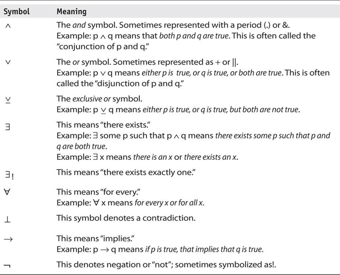
Table 4-1 is not an exhaustive list of all symbols in logic, but these are the most commonly used symbols. Make certain you are familiar with these symbols before proceeding with the rest of this section.
Several of these symbols are called connectives. That just means they are used to connect two propositions. Some basic rules for connectives are shown in Table 4-2.
TABLE 4-2 Connectives
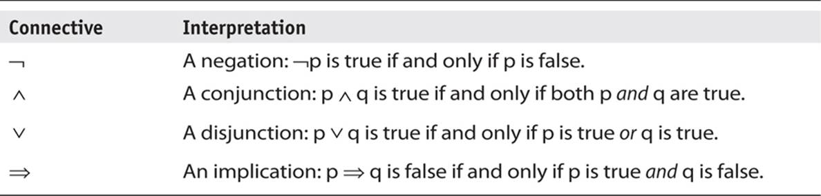
Here are a few basic facts about connectives:
![]() Expressions on either side of a conjunction are called conjuncts (p ∧ q).
Expressions on either side of a conjunction are called conjuncts (p ∧ q).
![]() Expressions on either side of a disjunction are called disjuncts (p ∨ q).
Expressions on either side of a disjunction are called disjuncts (p ∨ q).
![]() In the implication p ⇒ q, p is called the antecedent and q is the consequence.
In the implication p ⇒ q, p is called the antecedent and q is the consequence.
![]() The order of precedence with connectives is brackets, negation, conjunction, disjunction, implication.
The order of precedence with connectives is brackets, negation, conjunction, disjunction, implication.
Building Logical Constructs
Now that you are familiar with the basic concepts of deductive logic, and you know the essential symbols, let’s practice converting some textual statements into logical structures. That is the first step in applying logic to determine the veracity of the statements. Consider this sample sentence:
Although both John and Paul are amateurs, Paul has a better chance of winning the golf game, despite John’s significant experience.
Now let’s restate that using the language of deductive logic. First we have to break down this long statement into individual propositions and assign each to some variable:
p: John is an amateur
q: Paul is an amateur
r: Paul has a better chance of winning the golf game
s: John has significant golf experience
We can now phrase this in symbols:
(p ∧ q) ∧ r ∧ s
This sort of sentence does not lend itself easily to deducing truth, but it does give us an example of how to take a sentence and rephrase it with logical symbols.
Truth Tables
Once you have grasped the essential concepts of propositions and connectives, your next step is to become familiar with truth tables. Truth tables provide a method for visualizing the truth of propositions.
Here is a simple one. Keep in mind that the actual statement is irrelevant, just the structure. But if it helps you to grasp the concept, P is the proposition “you are currently reading this book.”
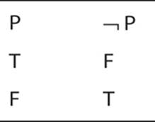
What this table tells us is that if P is true, then not P cannot be true. It also tells us that if P is false, then not P is true. This example is simple, in fact, trivial. All this truth table is doing is formally and visually telling you that either you are reading this book or you are not, and both cannot be true at the same time.
With such a trivial example, you might even wonder why anyone would bother using a truth table to illustrate such an obvious fact. In practice, you’d probably not use a truth table for this example. However, due to the ease most of you will have with comprehending the simple fact that something is either true or not, this makes a good starting point to learn about truth tables. Some of the tables you will see in just a few moments will not be so trivial.
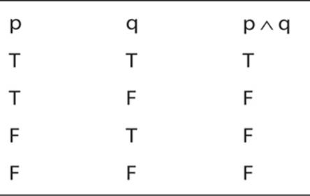
Now let’s examine a somewhat more complex truth table that introduces the concept of a conjunction. Again the specific propositions are not important. This truth table illustrates the fact that only if p is true and q is true, will p∧ q will be true.
What about a truth table for disjunction (the or operator)?
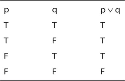
You can see that truth table shows, quite clearly, what was stated earlier about the or (disjunction) connective.
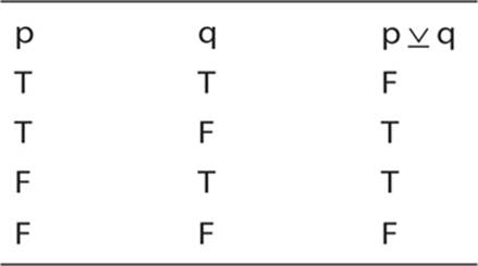
The exclusive or operation is also interesting to see in a truth table. Recall that we stated either p is true or q is true, but not both.
Next we shall examine implication statements. Consider p → q. This is read as p implies q.
Tip
The term implies, in logic, is much stronger than in vernacular speech. Here it means that if you have p, you will have q.
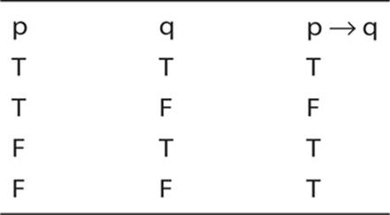
The previous truth tables were so obvious as to not require any extensive explanation. However, this one may require a bit of discussion:
![]() The first row should make sense to you. If we are stating that p implies q, and we find that p is true and q is true, then, yes, our statement p implies q is true.
The first row should make sense to you. If we are stating that p implies q, and we find that p is true and q is true, then, yes, our statement p implies q is true.
![]() The second row is also obvious. If p is true but q is not, then p implies q cannot be true.
The second row is also obvious. If p is true but q is not, then p implies q cannot be true.
But what about the last two rows?
![]() We are stating that p implies q; however, in row three we see q is true but p is not. Therefore not p implied q, so our statement that p implies q is not true.
We are stating that p implies q; however, in row three we see q is true but p is not. Therefore not p implied q, so our statement that p implies q is not true.
![]() In the fourth row, if have not p and not q, then p implies q is still true. Nothing in p being false and q being false invalidates our statement that p implies q.
In the fourth row, if have not p and not q, then p implies q is still true. Nothing in p being false and q being false invalidates our statement that p implies q.
Tip
Several sources can help you learn more about mathematical logic. A good one is the book Math Proofs Demystified by Stan Gibilisco (McGraw-Hill Education, 2005).
Combinatorics
Combinatorics is exactly what the name suggests: it is the mathematics behind how you can combine various sets. Combinatorics answers questions such as, how many different ways can you choose from four colors to paint six rooms? How many different ways can you arrange four flower pots?
As you can probably surmise, combinatorics, at least in crude form, is very old. Greek historian Plutarch mentions combinatorial problems, though he did not use the language of mathematics we use today. The Indian mathematician Mahavira, in the ninth century, actually provided specific formulas for working with combinations and permutations. It is not clear if he invented them or simply documented what he had learned from other mathematicians.
Combinatorics are used to address general problems, including the existence problem that asks if a specific arrangement of objects exists. The counting problem is concerned with finding the various possible arrangements of objects according to some requirements. The optimization problem is concerned with finding the most efficient arrangements.
Let’s begin our discussion with a simple combinatorics problem. Assume that you are reading this textbook as part of a university course in cryptography. Let’s also assume that your class has 30 students, and of those students, 15 are computer science majors and 15 are majoring in something else—we will call these “other.”
It should be obvious that there are 15 ways you can choose a computer science major from the class and 15 ways you can choose an other major. This gives you 15 × 15 ways of choosing a student from the class. But what if you need to choose one student who is either a computer science major or an other? This gives you 15 + 15 ways of choosing one student. You may be wondering why one method used multiplication and the other used addition. The first two rules you will learn about in combinatorics are the multiplication rule and the addition rule:
![]() The multiplication rule Assume a sequence of r events that you will call the events E1, E2, and so on. There are n ways in which a specific event can occur. The number of ways an event occurs does not depend on the previous event. This means you must multiply the possible events. In our example, the event was selecting one of the students, regardless of major. So you might select one from computer science or you might select one from other. The multiplication rule is sometimes called the rule of sequential counting.
The multiplication rule Assume a sequence of r events that you will call the events E1, E2, and so on. There are n ways in which a specific event can occur. The number of ways an event occurs does not depend on the previous event. This means you must multiply the possible events. In our example, the event was selecting one of the students, regardless of major. So you might select one from computer science or you might select one from other. The multiplication rule is sometimes called the rule of sequential counting.
![]() The addition rule Now suppose there are r events E1, E2, and so on, such that there are n possible outcomes for a given event, but further assume that no two events can occur simultaneously. This means you will use the addition rule, also sometimes called the rule of disjunctive counting. The reason for this name is that the addition rule states that if set A and set B are disjoint sets, then addition is used.
The addition rule Now suppose there are r events E1, E2, and so on, such that there are n possible outcomes for a given event, but further assume that no two events can occur simultaneously. This means you will use the addition rule, also sometimes called the rule of disjunctive counting. The reason for this name is that the addition rule states that if set A and set B are disjoint sets, then addition is used.
I find that when a topic is new to a person, it is often helpful to view multiple examples to fully come to terms with the subject matter. Let’s look at a few more examples of selecting from groups, illustrating both the addition rule (sometimes called the sum rule) and the multiplication rule (sometimes called the product rule).
What happens when you need to pick from various groups? Assume you are about to take a trip and you want to bring some along reading material. You have 5 history books, 3 novels, and 3 biographies. You need to select 1 book from each category. There are 5 different ways to pick a history book, 3 different ways to select a novel, and 3 different ways to choose a biography. The total possible combinations is 5 + 3 + 3. Why was addition used here? Because each choice can only be made once. You have 5 historical books to choose from, but once you have chosen 1, you cannot select any more. Now you have 3 novels to choose from, but once you have chosen 1, you cannot select any more.
Now let’s look at an example where we use the multiplication or product rule. Assume you have 3 rooms to paint and 4 colors of paint. For each room, you can use any of the 4 colors regardless of whether it has been used before. So you have 4 × 4 × 4 possible choices. Why use multiplication rather than addition? Because each choice can be repeated. Assume your 4 colors are green, blue, yellow, and red. You can use green for all 3 rooms if you want, or green for 1 room only, or not use green at all.
The multiplication rule gets modified if selection removes a choice. Supposed that once you have selected a color, you cannot use it again. In the first room you have 4 colors to select from, but in the next room only 3, and in the third room only 2 colors. So the number of possible combinations is 4 × 3 × 2. Selection removes a choice each time.
Selection with removal is actually pretty common. Here’s another example: Assume you want to line up 5 people for a picture. It should be obvious that you cannot reuse a person. Once you have lined up the 5 people, no more people are available for selection. So your possible combinations are 5 × 4 × 3 × 2 × 1.
Permutations
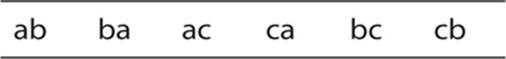
Permutations are ordered arrangements of things. Because order is taken into consideration, permutations that contain the same elements but in different orders are considered to be distinct. When a permutation contains only some of the elements in a given set, it is called an r-permutation. What this means for combinatorics is that the order of the elements in the set matters. Consider the set {a, b, c}. There are six ways to combine this set, if order matters:
![]() a b c
a b c
![]() a c b
a c b
![]() b a c
b a c
![]() b c a
b c a
![]() c a b
c a b
![]() c b a
c b a
Add one more letter to the set, {a, b, c, d}, and there are 24 possible combinations:
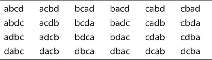
Fortunately, you don’t have to write out the possibilities each time to determine how many combinations of a given permutation there are. The answer is “n!”. For those not familiar with the n! symbol, it is the factorial symbol. The n! means n × n – 1 × n – 2 × n – 3, and so on. For example 4! is 4 × 3 × 2 × 1.
Consider ordering a subset of a collection of objects. If there is a collection of n objects to choose from, and you are selecting r of the objects, where 0 < r < n, then you call each possible selection an r-permutation from the collection. What if you have a set of three letters {a, b, c} and you want to select two letters. In other words, you want to select an r-permutation from the collection of letters. How many r-permutations are possible? Six:
What if our original collection was four letters {a, b, c, d} and you wanted to select a two-letter r-permutation? You would have 12 possibilities:
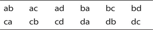
These examples should illustrate that the number of r-permutations of a set of n objects is n!/(n – r)!
To verify this, let’s go back to our first example of an r-permutation. We had a set of 3 elements and we wanted to select 2. And 3! is 3 × 2 × 1 = 6. The divisor (n – r)! is (3 – 2)!, or 1. So we have 6 r-permutations. In the second example, n = 4. And 4! = 4 × 3 × 2 × 1 = 24. The divisor (n – r)! is (4 – 2)!, or 2. So we have 12 r-permutations.
Clearly, we could continue exploring combinatorics and delving further into various ways to combine subsets and sets. But at this point, you should grasp the basic concepts of combinatorics. This field is relevant to cryptography in a variety of ways, particularly in optimizing algorithms. (On a personal note, I have found combinatorics to be a fascinating branch of discrete mathematics with numerous practical applications.)
Tip
Combinatorics is a very fascinating topic. The book Introductory Discrete Mathematics by V. K. Balakrishnan (Dover Publications, 2010) provides a good chapter on the topic as well as discussions of many other topics covered in this chapter.
Graph Theory
Graph theory is a very important part of discrete mathematics. It is a way to examine objects and the relationships between those objects mathematically. Put formally, a finite graph G(V, E) is a pair (V, E), where V is a finite set and E is a binary relation on V.
Now let’s examine that definition in more reader-friendly terms. A graph starts with vertices or nodes, what I previously referred to as objects. These objects can be anything. The edges are simply lines that show the connection between the vertices. There are two types of graphs: directed and undirected. In a directed graph, the edges have a direction, in an undirected graph, the edges do not have a direction. The edges are ordered pairs and not necessarily symmetrical. This simply means that the connection between two vertices may or may not be one-way.
Here’s an example. Consider two friends, John and Mike. Their relationship, shown in Figure 4-2, is symmetrical. They are each a friend to the other:

FIGURE 4-2 Symmetrical graph
If we use a graph to illustrate the relationship of a student to a professor, the relationship is not symmetrical, as shown in Figure 4-3.

FIGURE 4-3 Asymmetrical graph
The graph shown in Figure 4-3 is a directed graph—that is, there exists a direction to the relationship between the two vertices. Depending on what you are studying, the direction could be either way. For example, if you want to graph the dissemination of knowledge from the professor, then the arrow would point toward the student, and several students would likely be included.
You have already seen the terms vertex and edge defined. Here are a few other terms I need to define before proceeding:
![]() Incidence An edge (directed or undirected) is incident to a vertex that is one of its end points.
Incidence An edge (directed or undirected) is incident to a vertex that is one of its end points.
![]() Degree of a vertex Number of edges incident to the vertex. Nodes of a directed graph can also be said to have an in degree and an out degree. The in degree is the total number of edges pointing toward the vertex. The out degree is an edge pointing away, as shown in Figure 4-3.
Degree of a vertex Number of edges incident to the vertex. Nodes of a directed graph can also be said to have an in degree and an out degree. The in degree is the total number of edges pointing toward the vertex. The out degree is an edge pointing away, as shown in Figure 4-3.
![]() Adjacency Two vertices connected by an edge are adjacent.
Adjacency Two vertices connected by an edge are adjacent.
![]() Directed graph A directed graph, often simply called a digraph, is one in which the edges have a direction.
Directed graph A directed graph, often simply called a digraph, is one in which the edges have a direction.
![]() Weighted digraph This is a directed graph that has a “cost” or “weight” associated with each edge. In other words, some edges (that is, some relationships) are stronger than others.
Weighted digraph This is a directed graph that has a “cost” or “weight” associated with each edge. In other words, some edges (that is, some relationships) are stronger than others.
![]() A complete graph This graph has an edge between each pair of vertices. N nodes will mean N × (N – 1) edges.
A complete graph This graph has an edge between each pair of vertices. N nodes will mean N × (N – 1) edges.
Once you understand the basic concept of graphs and the relationship between vertices and edges, the next obvious question is, how can you traverse a given graph? This question can be answered in one of several ways. Let’s consider the graph shown in Figure 4-4, which has five vertices and seven edges.
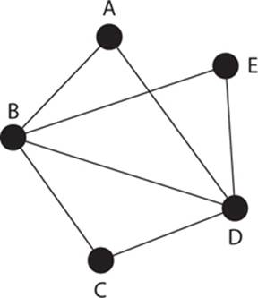
FIGURE 4-4 Traversing a graph
You can traverse a graph in three basic ways:
![]() Path With a path, no vertex can be repeated—for example, a-b-c-d-e. You can repeat an edge if you want, but not a vertex.
Path With a path, no vertex can be repeated—for example, a-b-c-d-e. You can repeat an edge if you want, but not a vertex.
![]() Trail A trail is the opposite of a path: no edge can be repeated—for example, a-b-c-d-e-b-d.
Trail A trail is the opposite of a path: no edge can be repeated—for example, a-b-c-d-e-b-d.
![]() Walk There are no restrictions. For example, a-b-e-d-b-c.
Walk There are no restrictions. For example, a-b-e-d-b-c.
Whatever traversal method you use, if you end at the starting point, that is considered closed. For example, if you start at vertex b and end at b, then this is closed, whether you use a path, trail, or walk. The length of traversal is simply the count of how many edges you have to cross.
There are two special types of traversal:
![]() Circuit A closed trail (for example, a-b-c-d-b-e-d-a)
Circuit A closed trail (for example, a-b-c-d-b-e-d-a)
![]() Cycle A closed path (for example, a-b-c-d-a)
Cycle A closed path (for example, a-b-c-d-a)
This leads to a few other terms:
![]() Acyclic A graph wherein there are no cycles
Acyclic A graph wherein there are no cycles
![]() Tree A connected, acyclic graph
Tree A connected, acyclic graph
![]() Rooted tree A tree with a “root” or “distinguished” vertex; the leaves are the terminal nodes in a rooted tree
Rooted tree A tree with a “root” or “distinguished” vertex; the leaves are the terminal nodes in a rooted tree
![]() Directed acyclic graph (DAG) A digraph with no cycles
Directed acyclic graph (DAG) A digraph with no cycles
Now you should have a basic idea of what a graph is and the different types of graphs. Rather than go deeper into the abstract concepts of graphs, I would like to answer a question that is probably on your mind at this point: What are graphs used for?
Graph theory has many applications. For example, they can help you determine what is the shortest (or longest) path between two vertices/nodes? Or what path has the least weight (as opposed to least length) between two vertices/nodes? If you reflect on those two questions for just a moment, you will see that there are clear applications to computer networks. Graph theory is also used to study the structure of a web site and connected clients. Problems in travel are obviously addressed with graph theory. There are applications in particle physics, biology, and even political science.
Tip
An excellent resource for a novice learning discrete mathematics is the book Discrete Mathematics Demystified by Steven Krantz (McGraw-Hill Education, 2008).
Conclusions
This chapter covered the basic mathematical tools you will need in order to understand cryptographic algorithms later in the book. In this chapter, you were introduced to number systems. Most importantly, you were given a thorough introduction to prime numbers, including how to generate prime numbers. The concept of relatively prime or co-prime was also covered. These are important topics that you should thoroughly understand and that are applied in the RSA algorithm.
You also saw some basic math operations, such as summation and logarithms, and were introduced to discrete logarithms. The discussion of modulus operations is critical for your understanding of asymmetric algorithms. The chapter concluded with an introduction to discrete mathematics, including set theory, logic, combinatorics, and graph theory. Each topic was briefly covered in this chapter; if you thoroughly and completely understand what was discussed in this chapter, it will be sufficient for you to continue your study of cryptography. The key is to ensure that you do thoroughly and completely understand this chapter before proceeding further. If needed, reread the chapter and consult the various study aids that were referenced.
Test Your Knowledge
1. Two vertices connected by an edge are __________.
2. The statement “Any number n ≥ 2 is expressible as a unique product of 1 or more prime numbers” describes what?
3. log327 = __________
4. A circuit is a closed __________.
5. Are the numbers 15 and 28 relatively prime?
6. A __________ is a group of numbers that are all congruent for some given modulus.
7. __________ is a deterministic test of primality that works on Mersenne numbers.
8. __________ are logarithms in respect to a finite group.
9. Set B is the __________ of set A if B has no elements that are also in A. This is symbolized as B = Ac.
10. __________ are ordered arrangements of things.
Answers
1. adjacent
2. The fundamental theorem of arithmetic
3. 3
4. trail
5. Yes
6. congruence class
7. The Lucas-Lehmer test
8. Discrete logarithms
9. complement
10. Permutations
Endnote
1. Edna E. Kramer, The Nature and Growth of Modern Mathematics, (Princeton University Press, 1983).
All materials on the site are licensed Creative Commons Attribution-Sharealike 3.0 Unported CC BY-SA 3.0 & GNU Free Documentation License (GFDL)
If you are the copyright holder of any material contained on our site and intend to remove it, please contact our site administrator for approval.
© 2016-2026 All site design rights belong to S.Y.A.