EnCase Computer Forensics (2012)
Chapter 7
Understanding, Searching For, and Bookmarking Data
EnCE Exam Topics Covered in This Chapter:
· Understanding data
· EnCase Evidence Processor
· Conducting basic searches
· Conducting advanced GREP searches
· Bookmarking your findings
· Organizing your bookmarks and creating reports
· Indexed searches
We’ve heard it said, and we’ll hear it said again: “It’s all about the 1s and the 0s.” Computers store or transmit data as strings of 1s and 0s in the form of positive and negative states or pulses. From that we get characters and numbers, all of which make up the data we find on computer systems. This chapter will begin with a review of binary numbers and their hexadecimal representations.
Once you understand how data is stored, you’ll then want to begin processing it. To help you do so, this chapter will cover the basics of the EnCase Evidence Processor, which is a new feature beginning with EnCase 7. It is, perhaps, more than just a feature; it’s a collection of case-preprocessing tools that will change your forensic workflow. Among those tools you will find the ability to index your data for later lightning-fast searches, plus the ability to conduct the more conventional raw searches using keywords.
Once you have a firm grasp of how data is stored and how to run the EnCase Evidence processor, the chapter will describe how to perform simple basic searches for that data. Then, you’ll step into the more advanced searching techniques known as GREP. GREP is a powerful search tool and one you need to master both for the examination and for everyday forensics.
Understanding data and locating it would not be beneficial if there were not some way of marking those findings and rendering them into some organized format that would later be generated into a report. EnCase has a powerful and, equally as important, flexible bookmarking and reporting utility.
The first aspect of your talent that your client or the prosecutor will see is your report. It needs to present well and read well. It will form the first, and maybe the last, impression they will have of your work and your capabilities. You can be the world’s sharpest and brightest forensics examiner, but if you can’t render your findings into an organized report that is easy to navigate, read, and understand, you will not do well in most aspects of this field.
More than a few times I’ve heard the comment that EnCase doesn’t have a very good reporting feature. I’m always taken aback by that remark. EnCase has, in my opinion, an excellent report-generating utility at several levels. Furthermore, the bookmark view provides many ways to organize and customize the report, which is probably the most flexible and customizable in the industry. Finally, you are given the option, at all levels of reporting, of generating an Rich Text Format (RTF) or web document.
In all fairness to that criticism, I am convinced, based on many ensuing discussions that followed this criticism, that the remark has its roots in lack of awareness of and training in using EnCase’s reporting utilities. It is time to close that knowledge gap. Because reporting your findings is a critical element to your success as a forensics examiner, Appendix A is devoted to that topic. In addition, the online resource that accompanies this book contains a downloadable sample report that you can use as a template or front end for your EnCase-generated report. This chapter also covers the basics of bookmark organization. Appendix A will pick it up from there and take you through the steps of creating a top-quality report.
This chapter concludes by covering indexed searching. This feature is new, starting with EnCase 6, and allows near-instantaneous search results once the index has been created. Creating the index will take time, but once done, the results will be worth the wait.
Understanding Data
In the following sections, I’ll cover binary data first, which is how 1s and 0s are rendered into human-readable characters and numbers. Following that discussion, I’ll cover the hexadecimal representation of binary data. Because 1s and 0s aren’t very readable or workable in their raw form, programmers have developed an overlay by which binary data can be viewed and worked with that’s much easier. It’s simply called hex.
I’ll wrap up the discussion of data with the ASCII table and how each character or decimal number therein is represented by a binary and hexadecimal value. Because computing has become global, the limits of the ASCII table mean that not all the world’s languages can be represented by 1 byte or 256 different characters. Accordingly, Unicode was born; 2 bytes are allotted for each character, making possible 65,536 different characters in a language. Therefore, I’ll also present an overview of Unicode.
Binary Numbers
Computers store, transmit, manipulate, and calculate data using the binary numbering system, which consists purely of 1s and 0s. As you may know, 1s and 0s are represented in many forms as positive or negative magnetic states or pulses. They can be lands or pits, light passing or not, pulses of light, pulses of electricity, electricity passing through a gate or not, and so forth. When you think about it, there are seemingly endless conditions where you can create a yes or no condition that can be in turn interpreted as a 1 or 0. Binary is absolute; it is a 1 or a 0. It is a yes or no condition without any maybes, although you can assemble a sufficient number of 1s and 0s arranged to spell “maybe!”
Binary numbers are arranged in organizational units. The smallest unit is a bit. A bit is a 1 or a 0 and is capable therefore of having only two possible outcomes. Two bits can have four possible outcomes, which are 00, 01, 10, or 11. Three bits can have eight possible outcomes, while 4 bits can have 16. Four bits is also the next unit and is called a nibble. Table 7-1 shows the possible number of outcomes, for up to 4 bits.
Table 7-1: Number of outcomes from 1 to 4 bits
|
Number of bits |
Number of outcomes |
Binary number |
|
1 (bit) |
2 |
0 or 1 |
|
2 |
4 |
00 01 10 11 |
|
3 |
8 |
000 001 010 011 100 101 110 111 |
|
4 (nibble) |
16 |
0000 0001 0010 0011 0100 0101 0110 0111 1000 1001 1010 1011 1100 1101 1110 1111 |
If I continued this table, I’d quickly fill the rest of the book—for every bit you add, you double the possible number of outcomes over the previous number. Mathematically, you are working with exponents or powers of 2, which are written as 20 = 1, 21 = 2, 22 = 4, 23 = 8, 24 = 16, and so on. The powers of 2, as previously noted, add up quickly, as shown in Table 7-2.
Table 7-2: Base-2 raised to powers from 0 to 128
|
Base number |
Power |
Decimal value |
|
2 |
0 |
1 |
|
2 |
1 |
2 |
|
2 |
2 |
4 |
|
2 |
3 |
8 |
|
2 |
4 |
16 |
|
2 |
5 |
32 |
|
2 |
6 |
64 |
|
2 |
7 |
128 |
|
2 |
8 |
256 (8 bits) |
|
2 |
9 |
512 |
|
2 |
10 |
1,024 (1 kilobyte) |
|
2 |
11 |
2,048 |
|
2 |
12 |
4,096 |
|
2 |
13 |
8,192 |
|
2 |
14 |
16,384 |
|
2 |
15 |
32,768 |
|
2 |
16 |
65,536 (16 bits) |
|
2 |
17 |
131,072 |
|
2 |
18 |
262,144 |
|
2 |
19 |
524,288 |
|
2 |
20 |
1,048,576 (1 megabyte) |
|
2 |
21 |
2,097,152 |
|
2 |
22 |
4,194,304 |
|
2 |
23 |
8,388,608 |
|
2 |
24 |
16,777,216 |
|
2 |
25 |
33,554,432 |
|
2 |
26 |
67,108,864 |
|
2 |
27 |
134,217,728 |
|
2 |
28 |
268,435,456 |
|
2 |
29 |
536,870,912 |
|
2 |
30 |
1,073,741,824 (1 gigabyte) |
|
2 |
31 |
2,147,483,648 |
|
2 |
32 |
4,294,967,296 (32 bits, number of possible outcomes with CRC) |
|
2 |
40 |
1,099,511,627,776 (1 terabyte) |
|
2 |
50 |
1,125,899,906,842,620 (1 exabyte) |
|
2 |
64 |
18,446,744,073,709,600,000 (64 bits) |
|
2 |
128 |
340,282,366,920,938,000,000,000,000,000,000,000,000 (128 bits, number of possible outcomes with MD5) |
![]()
Did you ever wonder why a hard drive is rated by the manufacturer as 30 GB and yet when you put it in your computer, it is only 27.9 GB? Many people think they have been shorted 2.1 GB and call tech support. It may also be raised as a question by opposing counsel wanting to know why EnCase didn’t see all of the drive. The answer could rest with an HPA or DCO, as previously discussed in Chapter 4. If, however, you are seeing all the sectors on the drive, an HPA or DCO is not the answer. The answer is, in part, found in Table 7-2. Note that the terms kilobytes, megabytes, gigabytes, terabytes, and exabytes were inserted at their respective locations. If a drive contains 58,605,120 sectors, it contains 30,005,821,440 bytes (multiply the number of sectors times 512 bytes per sector). A manufacturer, because it wants to paint its drive in the best possible light, uses base-10 gigabytes (1,000,000,000). The manufacturer simply moves the decimal point over nine places and rounds it off, calling it a 30 GB drive. Computers don’t care about marketing at all and work with a binary system, wherein 1 GB is 1,073,741,824 bytes (230). If you divide 30,005,821,440 by 1,073,741,824, you’ll find the answer is 27.94 and some change. Thus, your computer sees a drive with 30,005,821,440 bytes as having a capacity of 27.9 GB. EnCase reports the drive as having 27.9 GB as well. If opposing counsel asks where the missing 2.1 GB went, you can now explain it!
So far, I’ve covered a bit and a nibble (4 bits). The next organizational unit or group of bits is called a byte, which consists of 8 bits and is a well-known term. A byte also contains two 4-bit nibbles, called the left nibble and the right nibble. A byte can be combined with other bytes to create larger organizational units or groups of bits. Two bytes is called a word; 4 bytes is called a Dword (double word).
Dwords are used frequently throughout computing. The Windows registry, which will be covered in a later chapter, is full of Dword values. Because a Dword consists of 32 bits (4 bytes with each byte containing 8 bits), it is used frequently as a 32-bit integer. You’ll see plenty of Dwords in this business.
Larger than a Dword is the Qword or Quad word, which, as you might have guessed, consists of four words. Because a word is 2 bytes, four words consist of 8 bytes. Because a byte consists of 8 bits, 8 bytes (Qword) contains 64 bits. You’ll encounter more Dwords than Qwords, but Qwords are out there, and you need to be at least familiar with the term and its meaning.
Table 7-3 shows these various bit groupings and their properties. These are terms you should understand well because they are part of the core competencies that an examiner should possess. Advanced computer forensics deals with data at the bit level. Before attending advanced training, it is a good idea to review these concepts so they don’t hold you back and, better yet, so you can move forward with a firm grasp of the subject matter.
Table 7-3: Names of bit groupings and their properties
|
Name |
Bits |
Binary |
|
Bit |
1 |
0 |
|
Nibble |
4 |
0000 |
|
Byte |
8 |
0000-0000 (left and right nibbles) |
|
Word |
16 |
0000-0000 0000-0000 |
|
Dword (Double Word) |
32 |
0000-0000 0000-00000000-0000 0000-0000 |
|
Qword (Quad Word) |
64 |
0000-0000 0000-00000000-0000 0000-00000000-0000 0000-00000000-0000 0000-0000 |
The byte is a basic data unit, and understanding how it is constructed and evaluated is an important concept. From the previous discussion, you know that it consists of 8 bits and that it has two 4-bit nibbles, which are the left nibble and the right nibble. Figure 7-1 shows the basic byte, with a left and right nibble each consisting of 4 bits, for a total of 8 bits.
Figure 7-1: A byte consists of 8 bits subdivided into two nibbles, each containing 4 bits; they are known as the left and right nibbles.
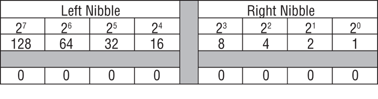
Recall that there are 256 possible outcomes for 8 bits or 1 byte. Thus, when a byte is being used to represent an integer, 1 byte can represent a range of decimal integers from 0 to 255, or 256 different outcomes or numbers.
If you look at Figure 7-1, you see that each of the eight positions (8 bits) has a value in powers of 2. Also shown is their decimal value. The least significant bit is at the far right and has a decimal value of 1. The most significant bit is at the far left and has a value of 128. If you add all the decimal numbers, you find they have a value of 255. By turning the bits on (1) or off (0) in each of these positions, the byte can be evaluated and rendered into a decimal integer value ranging from 0 to 255.
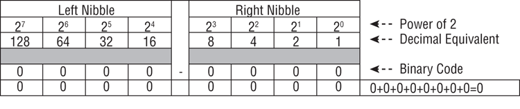
To demonstrate how this works, Figure 7-2 shows how this evaluation is carried out for the decimal integer 0. For the values represented by each bit position to equal 0, all must be 0, and all bits are set for 0. This is fairly simple to grasp and is, therefore, a good place to start.
Figure 7-2: All bits are set to 0. All decimal values are 0 and add up to 0.
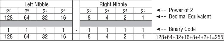
At the other extreme is 255. When you add all the decimal numbers, their total was 255. Thus, to represent the decimal integer 255, all bits must be on, or 1. Figure 7-3 shows a binary code for a byte with all bits on. When you add the numbers in each position where the bit is on, the total is 255.
Figure 7-3: All bits are on, or set to 1. Each bit position’s decimal value is added, and since all are on, the value is 255.
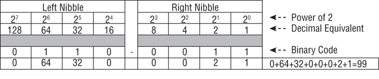
Since you’ve visited the two extremes, let’s see what happens somewhere in between. If you evaluate the binary code 0110-0011, as shown in Figure 7-4, you see that the bits are on for bit positions representing 64, 32, 2, and 1. The others are off and return a 0 value. If you add these numbers in the positions where the bits are on, you find that this binary code represents the decimal integer 99.
Figure 7-4: Evaluating binary code 0110-0011, we find bits on for bit positions 64, 32, 2, and 1. Adding those numbers returns a decimal integer value of 99.
The system is fairly simple once you understand the concept and therefore demystify it. Using this analysis method, you can determine the decimal integer value for any byte value. Admittedly, a scientific calculator is much faster, but you will eventually encounter analysis work where you must work at the bit level, and understanding what is occurring in the background is essential for this work.
Hexadecimal
Working with binary numbers is, with practice, fairly simple. You can see, however, that the numbers in the left nibble are a little too large to easily add in your head. Back in the beginning of computing, programmers apparently felt the same way, so they developed a shorthand method of representing and working with long binary numbers. This system is called hexadecimal (most people simply call it hex). You’ve no doubt heard of or used hex editors. EnCase has a hex view for viewing raw data, and as a competent examiner, you need to be well versed in hex.
A hexadecimal number is base-16 encoding scheme. Base-16 stems from the number of possible outcomes for a nibble, which is 16. Hex values will usually be written in pairs, with the left value representing the left nibble and right value representing the right nibble. Each nibble, evaluated independently, can have 16 possible outcomes and can therefore represent two separate numbers ranging from 0 to 15. To represent these decimal values with a one-character limit, the coding scheme shown in Table 7-4 was developed and standardized.
Table 7-4: Hexadecimal values and their corresponding decimal values
|
Decimal |
Hexadecimal |
|
0 |
0 |
|
1 |
1 |
|
2 |
2 |
|
3 |
3 |
|
4 |
4 |
|
5 |
5 |
|
6 |
6 |
|
7 |
7 |
|
8 |
8 |
|
9 |
9 |
|
10 |
A |
|
11 |
B |
|
12 |
C |
|
13 |
D |
|
14 |
E |
|
15 |
F |
Using this system of encoding, you can express the decimal values from 0 to 15 (16 different numbers or outcomes) using only one character. Because each nibble evaluated alone can have a maximum decimal value of 15, you have a system where you can have one character to represent the decimal value of each nibble. Figure 7-5 shows how this works when each nibble is evaluated independently using the hex encoding scheme. In the figure, a hex value of 98 means the left nibble has a decimal value of 9 and the right nibble has a decimal value of 8.
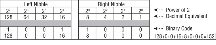
Using this system, you have a shortcut method for expressing the binary code 1001-1000, which is hexadecimal 98. This is usually written as 98h to differentiate it from the decimal number 98. Using the previous method of evaluating the decimal value of this same byte, as shown in Figure 7-6, we determine that the bits are on for bit positions 128, 16, and 8. Adding these together, you find that the decimal value for this same binary coding is 152. Thus, 98h, decimal 152, and binary 1001-1000 are all equal values, just expressed differently (base-16, base-10, and base-2).
Figure 7-5: The hexadecimal encoding scheme at work. The left nibble has bits on for 8 and 1 and has a value of 9. The right nibble has bits on for 8 only and has a value of 8. Thus, this binary coding (1001-1000) would be expressed in hexadecimal format as 98, or 98h.
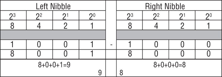
Figure 7-6: The same binary coding shown in the previous figure evaluated as a decimal value. The bits are on for bit positions 128, 16, and 8, which total 152 for the decimal value.
![]()
You may also see hex denoted another way, which is with 0x preceding it. For example, 98h could also be written as 0x98. This method finds its roots in some programming languages (C, C++, Java, and others), where the leading 0 tells the parser to expect a number and the x defines the number that follows as hexadecimal. So, to keep things simple, I’ll use the suffix h to denote hex, but you will see it in other publications using the other method.
To test your understanding of hexadecimal encoding, let’s try a couple more examples using simple logic and not diagrams. At the very outset, you saw the example, in Figure 7-3, of all bits being on, meaning you add all the bit position decimal values and arrive at a decimal value of 255. Without resorting to diagramming, you can easily convert this to a hexadecimal value just using some logic. With all 8 bits on (1), each nibble’s 4 bits are likewise on when you evaluate them independently. When a nibble’s bits are all on, all the nibble’s bit positions are totaled and they equal 15. Thus, each nibble’s decimal value is 15. The hex encoding for decimal 15, according to Table 7-4, is F. So, each nibble’s hex value is F, and, combined, they are FF.
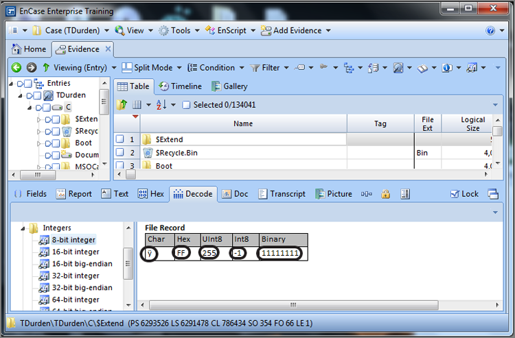
Figure 7-7 shows an EnCase hex view in which FFh has been bookmarked and viewed as an 8-bit integer. Its binary coding (1111-1111) is shown as well as its decimal value of 255 and its hex value of FF. Not yet discussed is another interpretation of this data, which is as a signed integer with a value of -1. Further, this value has a character represented by it as well, which is ÿ (y with two dots over it). We will cover the ASCII table in the next section, and the character issue will make better sense.
Let’s take that logic one step further to arrive at a hex value for the decimal value 254. That is, in simple terms, 255 minus 1! If all bits are on for 255, to get 254 you need to turn off the bit for the bit position value of 1, which is in the rightmost position. Thus, 255 is binary 1111-1111, and 254 is 1111-1110. To convert this to hex, at a glance, you know the left nibble is still F because nothing changed there. The right nibble is 1 less than before and should be decimal 14 (8 + 4 + 2 + 0). From Table 7-4, you know the hexadecimal value of decimal 14 is E. Thus, the hexadecimal value for decimal 254 is FEh.
Figure 7-7: EnCase hex view of FF bookmarked and viewed as an 8-bit integer. Note the various interpretations of this data that are possible.
Characters
I mentioned that FFh, in addition to representing a decimal integer value of 255, could also represent a character, which in this case was ÿ (y with two dots over it). When data is stored or used by a program, the program defines the type of data it is. Without getting too involved in programming terminology, data can be text, integers, decimals, and so forth. Let’s focus on text data.
ASCII
If the data is in a text format, the characters to be displayed are derived from a standard chart called the ASCII chart. This stands for the American Standard Code for Information Interchange and was created by Robert W. Bemer in 1965 to create a standard for interchange between the emerging data-processing technologies.
In the simplest of terms, the chart maps characters and escape codes to binary or hexadecimal values. If everyone uses the same mapping scheme, then when the text letter A is needed, 41h is used, and everyone with the same mapping system can read the letter A correctly since they are all using the same character mapping scheme.
Using this system, 7 of the 8 bits are used to create a table of 128 letters, numbers, punctuation, and special codes. Seven bits provides for 128 different outcomes or characters. This portion of the table (0-127) is called the ASCII table. It is sometimes called low or low-bit ASCII.
![]()
As much of this data is transmitted, the eighth bit is a parity bit and is used for error checking to determine whether an odd or even number of binary 1 bits were sent in the remaining 7 bits. The sending and receiving units have to “agree” or be in sync with the same odd or even parity scheme. When that is established, the sender sends a parity bit, and the receiver uses the sent parity bit to validate the received data. However, it is rarely used anymore because other, more reliable and sophisticated error checking systems have evolved. Besides that, we needed to use that extra bit for more characters!
As computing evolved and encompassed more disciplines and languages, additional characters were needed. When the PC was born in the early 1980s, IBM introduced the extended ASCII character set. IBM did away with the parity bit and extended the code to 8 bits, which provided twice the number of characters previously allowed with the 7-bit system. The new character set therefore provided 128 additional characters to the basic set. Most of these characters are mathematical, graphics, and foreign-language characters. This character set is also called the high-bit ASCII set.
You can find the complete set of ASCII character codes (low-bit and high-bit) on many websites, such as the following:
www.cpptutor.com/ascii.htm
If you will look over the entries, you will see them displayed in ascending decimal value order. Each line or item in this 256-character list has a decimal value, a hexadecimal value, and a character code. Since everything is stored in binary, as 1s and 0s, the list includes each character’s binary coding as well.
Before moving away from the ASCII character codes, I’ll touch upon a couple of the finer points that can help if well understood and possibly impede if not understood. The first point is that uppercase and lowercase letters are represented by entirely different code. An uppercase E is 45h, while a lowercase e is 65h. When I start covering searching for data, the concept of case-sensitive searching will emerge, where searching for 45h is different from searching for 65h. I’ll get into that in detail soon enough. For now, just recognize that the two are different.
Understanding that upper- and lowercase letters are different is easy. What may be confusing are numbers. If I type the number 8 and it is stored as text, then 8 will be represented as 38h. But if the integer value of 8 is being stored for some math function, then it is likely stored as 08h since its data type is no longer text. Conversely, sometimes you will see what appear to be characters in the middle of gibberish when you are viewing binary data in text view. In these cases, EnCase is looking at binary data through the ASCII character set, and when hex values correspond with printable ASCII characters, they are rendered as such even though they really aren’t text.
If numbers aren’t confusing enough, sometimes you will find numbers stored as ASCII characters, while those same numbers are stored elsewhere as integers. A good example of this would be IP addresses. Sometimes the program will store an IP address as 128.175.24.251, which is pure human-readable ASCII text. Another program may store this IP in its integer form, which is the way the computer actually uses it. This same IP would read 80 AF 19 FB. In this method, each of the four octets of an IP address is represented by a single byte or 8-bit integer. Using the previous plain-text IP address, decimal 128 is 80h, decimal 175 is AFh, decimal 24 is 19h, and decimal 251 is FBh. Other programs, such as KaZaA, iMesh, and Grokster, sometimes store this same IP as FB 19 AF 80, which is the reverse order (little endian).
To summarize, the hex string 54 45 58 54 could be interpreted in several ways, depending on the context in which it is used and stored on the computer. As a 32-bit integer, it would represent a value of 1,413,830,740. As four separate 8-bit integers (as an IP address could be stored), it would stand for the IP address 84.69.88.84. If this string were found in KaZaA data, it would represent the IP address 84.88.69.84. Finally, if it were found in the middle of a string of text, it would stand for the word TEXT, spelled in all uppercase letters.
As you progress in the field, interpreting text and hex values will become second nature. Text will usually quite obviously be text when you see it. When you have to interpret integers, you’ll usually be following an analysis guideline that describes where and how a certain piece of data is stored. You may, however, be conducting research in which you are reverse-engineering a data storage process. Under those conditions, you are flying blind, using trial and error to determine how data is stored and what it means forensically. For now, just remember that data can be interpreted in different ways, depending on the program and the context in which it is being used.
Unicode
As computing became global and the limits imposed by a 256-character code set could not accommodate all the characters in some languages, a new standard had to emerge. Unicode was the answer to this challenge. Unicode is a worldwide standard for processing, displaying, and interchanging all types of language texts. This includes character sets previously covered by the ASCII set (mostly the Western European languages). Unicode characters also allow for languages that use pictographs instead of letters, which are primarily the Eastern country languages, such as Chinese, Japanese, and Korean.
To encompass such a broad set of characters, Unicode uses 2 bytes per character instead of 1 byte. Unicode was introduced into EnCase version 4 and allows processing of any language for which there is an established code page or character set, which covers most of the world’s written languages.
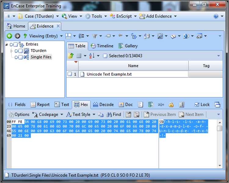
Although many languages don’t require Unicode to render their character sets, many store text in Unicode. Sometimes they store the same text in ASCII and in Unicode simultaneously. The letter A in ASCII, as you’ll recall, is 41h. The letter A in Unicode is 4100h. Searching for 41h is different from searching for 4100h. When I begin the discussion on searching, you’ll want to remember the differences between ASCII and Unicode. Because considerable data is stored in Unicode, unless you have a good reason not to, you’ll want to search for your data in both formats, ASCII and Unicode. Figure 7-8 is an EnCase view showing a string of text that is stored in a Unicode format.
Figure 7-8: Text string stored in Unicode. Note the 00 after each character.
EnCase Evidence Processor
The EnCase Evidence Processor is a collection of tools that carry a series of routines necessary to the proper examination of evidence. It is best described as a highly configurable preprocessing tool. Before we start using this tool, we must first make certain we have followed several steps that constitute best practices, namely:
1. Allow EnCase to complete the evidence verification process.
2. Check the verification report to ensure that the verification completed with zero errors and that the acquisition and verification hashes match.
3. Determine the time zone settings for the various evidence items.
4. Adjust EnCase to reflect the time zone offsets as needed; otherwise, EnCase, by default, will assign the time zone offset of the examination workstation.
![]()
If there are deleted partitions, you’ll want to recover them before running the EnCase Evidence Processor.
I previously discussed evidence verification and how to check for successful verification. If you are unsure, you can review the material on this topic in Chapter 5.
As most file systems store data in GMT and display it in local time, it is usually a better practice to display and report time in the local offset. There are, of course, exceptions. A good example would be examining several devices in the same case that were in different time zones. In those cases, it is better to view them all in one time zone. Regardless, you need to know which time zone offset is configured for each device. In Windows, this information is stored in the registry, specifically at HKLM\System\ControlSet001\Control\TimeZoneInformation\TimeZoneKeyName. You should take note that the current control set will vary and that “001” will not always be the current set. We’ll show you how that determination is made as well.
Before we examine the registry, we first have to navigate to the registry hive file in question, which is located at \Windows\System32\config\SYSTEM. There are other hive files in this folder, but for now we are concerned only with this particular one. Registry hive files are compound files that can be parsed and displayed in a hierarchical format, which is also called mounting the file in EnCase. To do so, place your cursor on the parent folder in the Tree pane, which forces the child objects to display in the Table pane, as shown in Figure 7-9. In the Table pane, you highlight the registry hive file named SYSTEM. On the Evidence tab toolbar, open the Entries menu and select View File Structure. You will next see a dialog box, as shown in Figure 7-10. Accept the defaults and click OK.
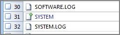
EnCase will take a few minutes to parse the hive file and display the results. You can see the progress bar in the lower-right corner. When done, you will notice that the hive file has turned blue, indicating it is now hyperlinked and also has a plus sign on it, as shown in Figure 7-11.
Figure 7-9: Parent folder is selected in the Tree pane. The hive file is highlighted in the Table pane. The View File Structure tool is then selected from the Entries menu.
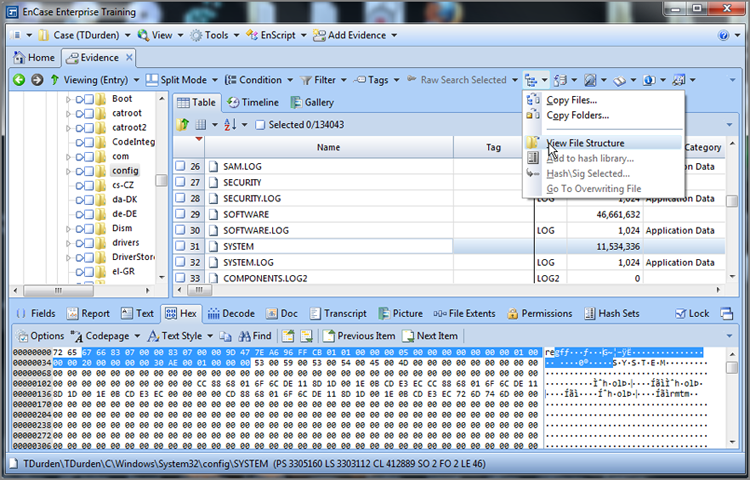
Figure 7-10: View File Structure dialog box from which options can be selected. The defaults are fine for getting the time zone offset.
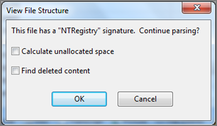
Figure 7-11: SYSTEM hive is blue (hyperlinked) and has a plus sign on the icon, both of which indicate it has been mounted and can be viewed.
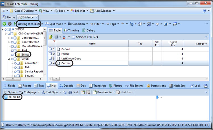
Since the SYSTEM hive file is now hyperlinked, simply click it, and it will open into its own viewing pane, as shown in Figure 7-12. To determine which control set is the current control set, we must look to the Select key and the value Current, both of which are circled in Figure 7-12. By highlighting Current in the Table pane, we can view its value in the View pane below, which can best be viewed in the Hex tab. Its value, in this case, is 01, which means ControlSet001 is the current control set.
Figure 7-12: Select key is showing the Current Control Set to be number 01.
Knowing that, in this case, ControlSet001 is the current control set, we next drill down into this key until we locate the value TimeZoneKeyName, as shown in Figure 7-13. In this case, we see that the time offset is Pacific Standard Time (PST). Before we leave this key (TimeZoneInformation), we need to make certain that the Dynamic Daylight Time disable function hasn’t been activated. This value is located under the TimeZoneInformation key and is named DynamicDaylightTimeDisabled. Normally, the Dynamic Daylight Time adjustment is enabled such that when daylight saving time is in effect, the time automatically adjusts. The registry is loaded with double negatives, which in this case disabled with a zero value means enabled, which is the default value and is shown in Figure 7-14.
At this point, we know how to determine the current control set, the time zone name, and whether the Dynamic Daylight Time adjustment is enabled or not. In our case, Pacific Standard Time is the offset, and automatic adjustment occurs for daylight saving time. Let’s put this information into EnCase for the device in question. To do so, we go back to the Entries view and in the Tree pane, highlight the root, forcing the device to appear in the Table pane, where we highlight it, as shown in Figure 7-15.
Figure 7-13: TimeZoneKeyName value indicates Pacific Standard Time.
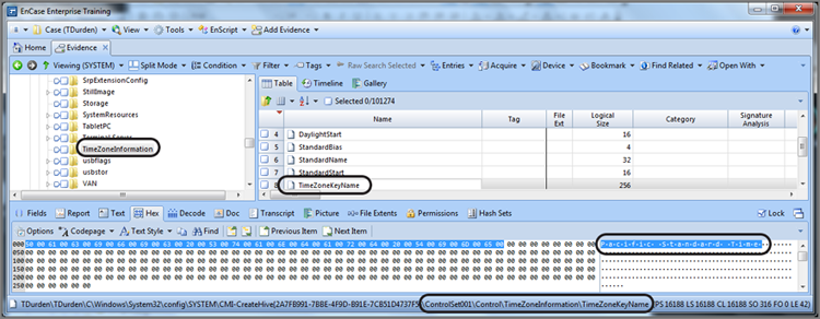
Figure 7-14: DynamicDaylightTimeDisabled is zero, meaning that the Dynamic Daylight Time adjustment is enabled.
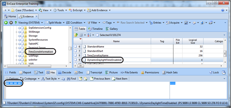
Figure 7-15: Modifying time zone settings
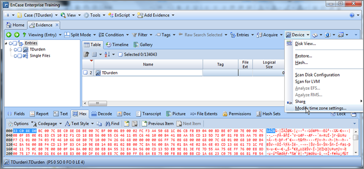
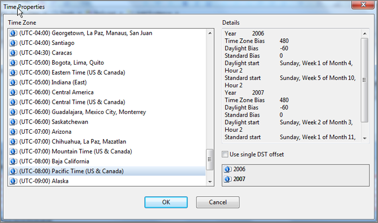
With the device highlighted in the Table pane, open the Device menu on the Evidence tab toolbar and select Modify Time Zone Settings, as shown in Figure 7-15. Because my examination machine was currently in the Central time zone, the default offset is Central Standard Time (CST). Since the evidence device was set to PST, we need to make an adjustment and change the offset to PST, as shown in Figure 7-16. When the correct time zone is selected, click OK, and the change is applied right away.
Figure 7-16: Changing time zone offset to Pacific Standard Time
At this point, you have carried out your best practices by verifying your evidence acquisition and setting the proper time zone offset to your evidence. You are now set to run the EnCase Evidence Processor. In essence, there are two basic requirements, which are that there must be evidence in your case to process, which stands to reason. If you are previewing a device, you’ll need to either acquire it first or make the acquisition a part of the evidence processing, which you’ll soon see. Later versions of EnCase 7 are planned to allow for select processing of previewed evidence, such as running modules we will cover shortly. For the full power of processing, including indexing, you will want to acquire the evidence first.
![]()
Beginning with EnCase 7.03, the EnCase Evidence Processor may be run on previewed devices.
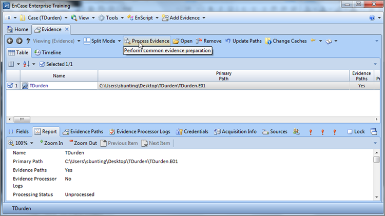
The EnCase Evidence Processor can be run from the Home screen or from the Evidence tab. We’ll run it from the Evidence tab because that will likely be the most convenient location from which to run the tool. From the Evidence tab, select the evidence items you want to process and launch the EnCase Evidence Processor from the Evidence tab toolbar, as shown in Figure 7-17.
Figure 7-17: Running the EnCase Evidence Processor from the Evidence tab toolbar
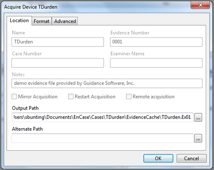
Once the EnCase Evidence Processor loads, the interface will appear, and you can change many options, as shown in Figure 7-18. As mentioned earlier, you can acquire as part of the processing. In the upper pane, the evidence in the case is shown. For each evidence item, you can choose to acquire and/or process. If you select to acquire an item, you’ll be presented with device acquisition menu that should look very familiar, as shown in Figure 7-19.
Figure 7-18: The EnCase Evidence Processor menu showing various options for processing
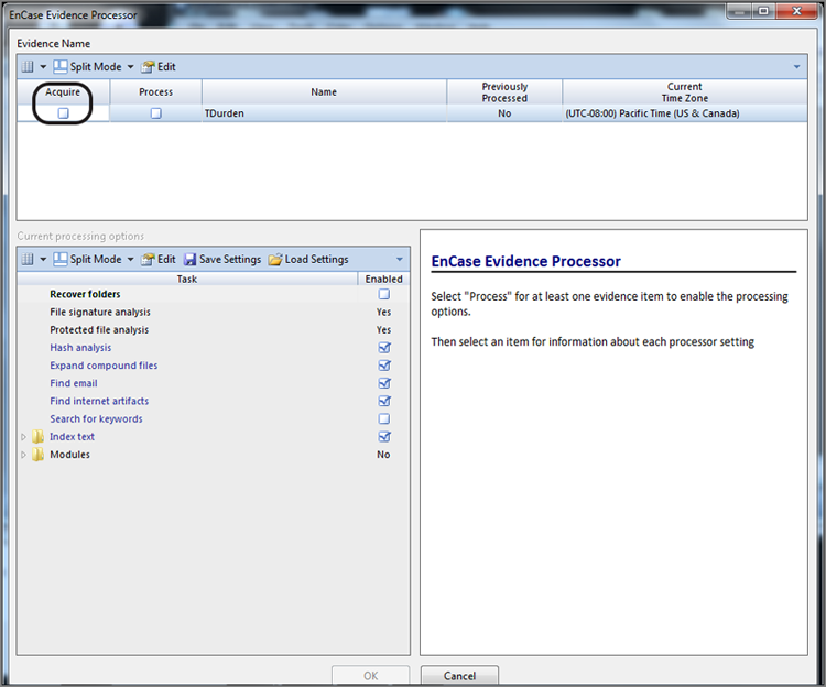
Figure 7-19: Upon choosing to acquire, you are immediately provided with a quite familiar menu.
You will note that until you select the Process check box, the processing options are not available; they are grayed out. Upon selecting Process, the options become available, as shown in Figure 7-20. You should make a careful observation of the red flags in Figure 7-20. Any item with a red flag must be run the first time the evidence processor is run and can’t be run in any subsequent runs. Any item without a red flag can be run during any subsequent runs of the processor.
Figure 7-20: Processing options become available when the Process check box is selected. Red flag items can be run only during the first run of the processor. Protected file analysis is now optional and may be activated or not.
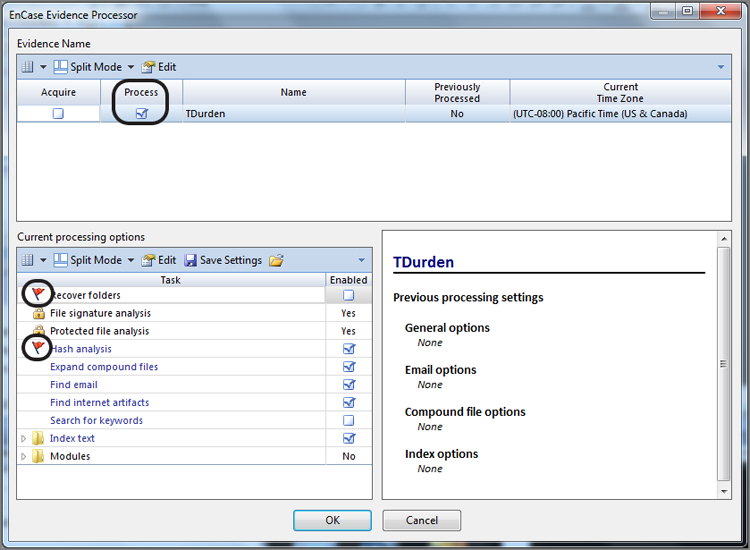
Recover Folders functions only for FAT and NTFS file systems. It is an option but has a red flag, meaning if you want to run it, you have to do so on the first run of the processor. Recover Folders is highly recommended, so you should run it unless you have a compelling reason not to, especially when you have only one chance to do so. File Signature Analysis and Protected File Analysis are locked and will run always. We’ll talk more about the results of these two items in later chapters.
Hash Analysis also has a red flag and must be run on the first run or not at all. Any item that turns blue (hyperlinked) when checked has options. The hash analysis options are MD5, SHA-1, or both. Expand Compound Files, because it lacks a red flag, can be run at any time. Their options are also very simple, which is only archives at the current time.
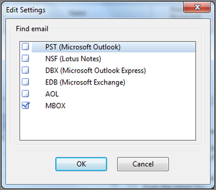
Email can be run at any time also. Options for email are many but are still rather simple, since you are only selecting the various types of email for EnCase to search. Figure 7-21 shows the various types of email that EnCase can find and parse. You can expect this list to expand as EnCase adds support for additional or new email types.
Figure 7-21: Find Email options
EnCase can find Internet history for the various common browser types. It can also be run during any subsequent run of the processor. Your only option will be to search unallocated spaces. The default is no unallocated search, so you’ll need to enable it for a comprehensive search.
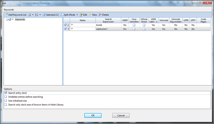
Searching for keywords can now be done as part of the case processor. Checking its box and opening the options provides a menu that veteran EnCase users will find quite familiar, as shown in Figure 7-22. In the next section, I cover the various types of keywords searches and their options.
Figure 7-22: Keywords menu options
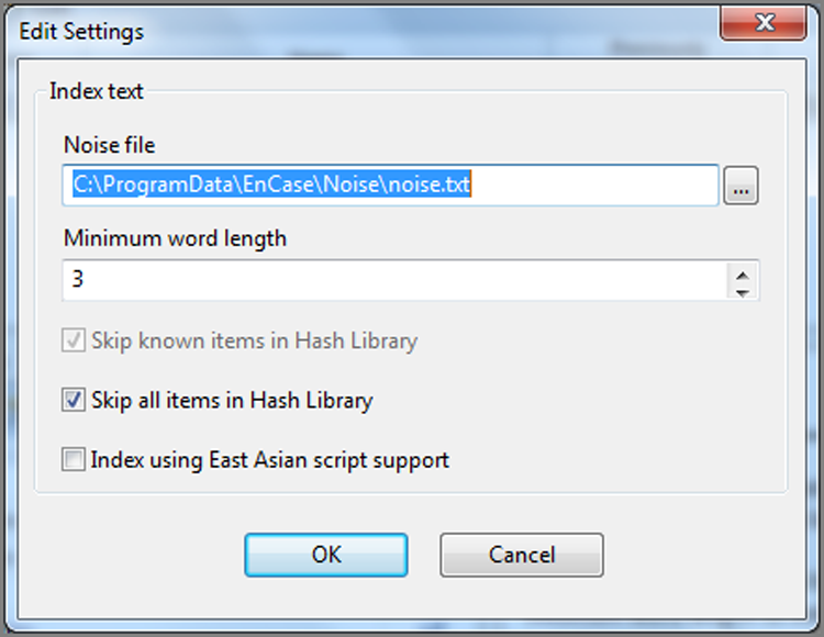
The next processing option is that of text indexing. This step requires considerable time to run, but the payoff is lightning-fast searches of the index later. Figure 7-23 shows the options for indexing. You can select a Noise File if you have one created. Its purpose is to eliminate certain common short words from index, thereby saving time and space. You can choose the minimum word length. Usually three letters is an ideal setting for words. Any fewer is simply bloat for the index. You have the option of skipping known items in the hash library, all items in the hash library, or neither. Finally, if East Asian languages are involved, you’ll need to select the option to include support for those languages.
Figure 7-23: Index text options
Under the text indexing option, there is an option for extracting personal information. The options are many, as shown in Figure 7-24, but are also quite self-explanatory. These include credit cards, phone number, email addresses, and Social Security numbers. You can also edit and create conditions to work with these options.
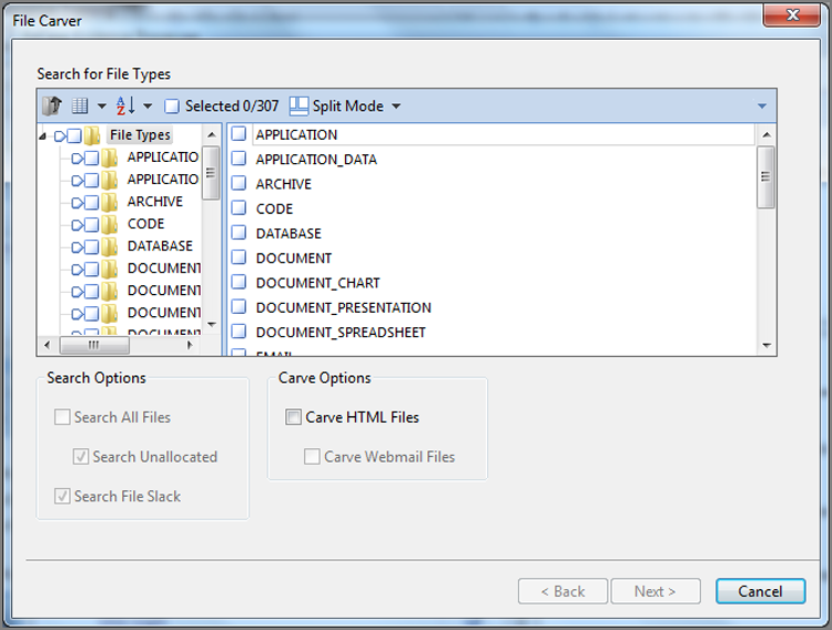
Several modules are available, and more will no doubt be added as this tool is enhanced. Figure 7-25 shows the various options currently available. All have extensive options available, and I suggest visiting each module’s option set to become familiar with the various features and capabilities. One of particular interest is the File Carver option, shown in Figure 7-26. The tool uses the data in the File Types database to facilitate file carving. In essence, any file type in the database can be carved, albeit some more successfully than others. You have the option to search all files, unallocated spaces, and/or file slack. You can also opt to carve HTML files and webmail files as a separate option outside the file types.
Figure 7-24: Personal information options
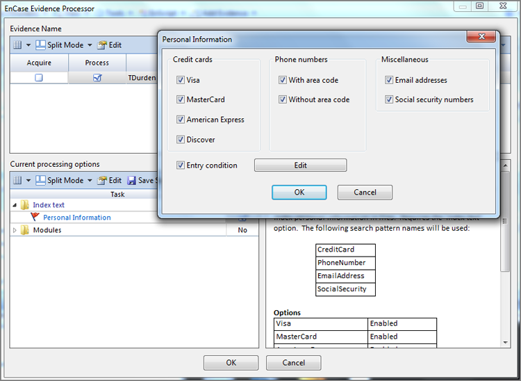
Figure 7-25: Processing modules available
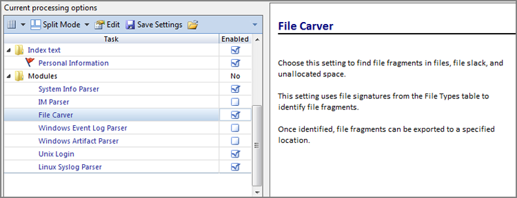
Figure 7-26: File carver options
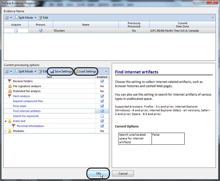
Once you have selected your options, you can click OK to run, as shown in Figure 7-27. If you prefer to save your evidence processor settings so that you don’t have to configure them each time or would prefer to at least have a base set, you can do so. At the top of the processing options there is a toolbar with menus, including Save Settings and Load Settings. As the names imply, you can save and load settings using this feature. Once the processor starts running, it will take hours, perhaps days, depending on the amount of data involved and the options selected.
We are often faced with too much data and too little time, in which there are demands for answers right away. Such situations require you to triage and make decisions about which data to process now and which data to process later. Clearly, you need to run the red flag items during the first run. You also need to determine what your case is all about and which items to process to give you the answer sooner rather than later. If your case is all about email, run your red flag items and Find Email (see Figure 7-20) during the first run. You can then start your analysis work on the initial results, and you can perform another subject processor run in the background while working.
When your case processor finishes, the results of the processing appear in many places. Some items appear on the Records tab while others appear in the Entries view of the Evidence tab. As I cover the various topics, I include in those discussions the results of the Evidence Processor. For now, it’s time to discuss keyword searching in depth.
Figure 7-27: Options selected and ready to run. Note the Save Settings and Load Settings options.
Searching for Data
EnCase provides for two basic methods for searching for data. One approach is that of using an indexed search. To do so, one must first create an index using the EnCase Evidence Processor, which we just covered. Searches are then conducted against the index, and results are nearly instantaneous. The other method of searching is that of raw searching, whereby keywords are created, and the entire stream of selected data is searched for strings matching those keywords. A related search method is the ability to search smaller sets of data while in the View pane. Each method has its time and place, with each having advantages and disadvantages. Indexed searching takes significant time to build an index but pays it back later with lightning-fast searches, including proximity searches, Boolean searches, and the like. Raw searches take time for each search, yet can be extremely precise or highly flexible when using GREP expressions. With experience, you know when to use which type.
![]()
As data sets have grown tremendously, indexed searching technologies have advanced to keep pace, to the point where indexed searching is usually the better choice. Further, many data types are compressed or otherwise obfuscated, such as PDF files, Office 2007, and newer formats (.docx, .xlsx, .pptx, and so on). Raw text searches against these file types are nearly useless. The index search in EnCase uses Outside In to extract the transcript text from the files, and this text is used in the index. Thus, indexed searching enables searching of files that would otherwise not yield fruit with traditional raw searches, and allows rapid searches across large sets of data. Also, to search many file types, such as Microsoft Office 2007 (and newer) files, PDFs, and the like, you must do so with an indexed search. For such file types, there is no searchable raw text. Rather, the text must first be extracted into transcript text and subsequently indexed. In short, unless you do an indexed search of Office 2007, newer file types (.docx, .xlsx, .pptx, and so on), and PDFs, you are going to miss data with your search.
In this chapter, I’ll discuss raw searches in EnCase. Using EnCase’s Raw Search All tool, you can search for keywords anywhere on the physical drive. You can search the entire case (all devices in the case) at once or any subset of data within the case, down to a single file. There is even a tool called Find that allows you to search within a block of selected text. This tool is covered in Chapter 6 and is available by selecting a right-click option, by choosing a menu, or by pressing Ctrl+F in the View pane while in the Text or Hex view.
Next, I’ll cover how to create keywords. I’ll discuss your options when conducting a search. Then I’ll discuss GREP, which means “Globally search for the Regular Expression and Print.” This tool comes from the Unix domain and is powerful for constructing searches. It allows you to be extremely focused or very broad, as the situation warrants.
Creating Keywords
You can’t conduct a search without first creating a string of characters for the search engine to find. In EnCase, those search strings are called keywords.
Keywords and Keyword Files
Keywords, once created, are stored in a file for later use. Up through and including EnCase 3, keywords were stored in the case file and were case specific (unless exported and transferred manually to another case). With EnCase 4, keywords became a global resource and were stored separately in a global KEYWORDS.INI file. Starting with EnCase 5, the best of both worlds were combined, and keywords can be either global (stored in the KEYWORDS.INI file) or case specific (stored in the case file).
The concept of local and global keywords disappears somewhat with EnCase 7, at least within the interface. First, you must consider that you can, as you recall, run a raw keyword search from within the EnCase Evidence Processor. If you do so, the keywords will be stored within the device’s cache files and can be used whenever the device is searched.
The other method or location of invoking the raw keyword search is from the toolbar of either the Evidence tab’s Table tab or its Entries tab. If the former (Table tab), you will be raw searching all evidence devices. If the latter (Entries tab), you will be raw-searching based on the selections made in the Tree pane. When you conduct a raw search from the Evidence tab toolbar, the keywords are either loaded from or saved to a file. This file will contain keyword sets for your given search and are stored in files with the extension .keyword. Where you opt to store them is the only indicator of whether they are local or global. You create a keyword or keywords and then name the file in which they will be stored. In this manner, keywords can be grouped in as many files as you deem appropriate and are likewise stored where you deem appropriate. Once we start creating keywords, you will see how this works. For now, let’s get started by creating keywords for a raw search.
Creating Keywords
To create a raw search keyword, you must first decide at which level you will conduct your search. If you are going to search all evidence devices, you can launch the search from the Table tab of the Entries view of the Evidence tab. In fact, from this location, you can only search everything. If you want to search a limited set of data, go to the Entries tab of the Evidence tab and select the items to search from the Tree and Table panes. From this location, you can also select all by placing a blue check mark at the root of the case in the Tree pane. If you are going to use blue check marks to select a limited data set for searching, it is a best practice to first check the Dixon box and reset it to zero (click in it once) before making selections. Otherwise, your search selection will be in addition to that which was previously selected. Figure 7-28 shows that two sets of user files have been selected in the Tree pane, with the Dixon box reflecting 3,623 files selected.
Figure 7-28: Files selected for search
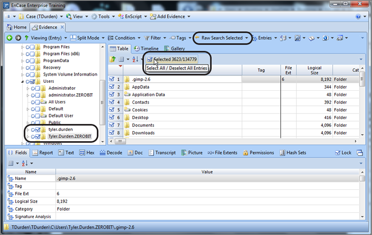
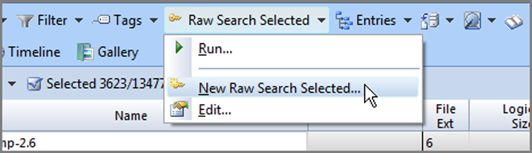
Thus far, we’ve selected the files that we want to search. Now it’s time to create a keyword, configure the various search options, and then launch the search. In Figure 7-28, you can see that the Raw Search Selected menu on the toolbar has been circled. Click on this menu, and choose New Raw Search Selected, as shown in Figure 7-29.
Figure 7-29: Raw Search Selected menu options
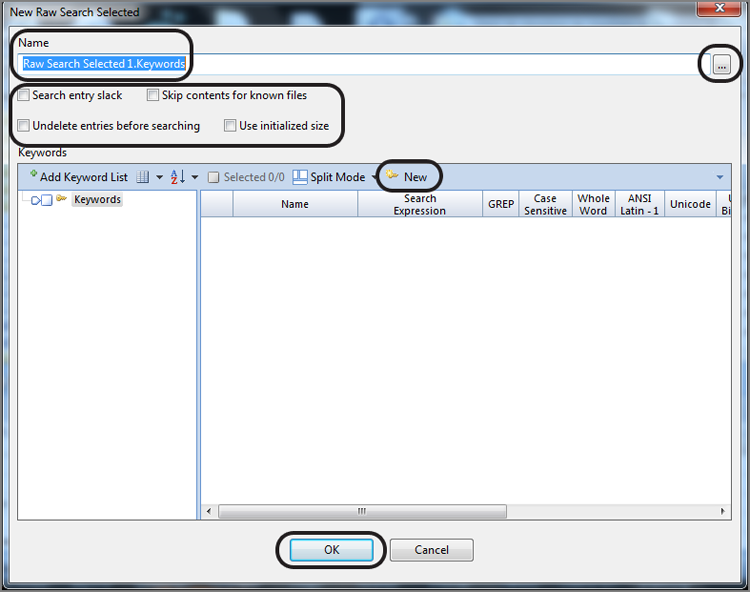
The New Raw Search Selected dialog box will appear next. Veteran EnCase users will be familiar with most of the menu features, as shown in Figure 7-30. It is important to note that this menu both creates or loads the keyboards and also launches the search when you click OK. You can see many options relating to the search, such as Search Entry Slack, User Initialized Size, and so on, appearing in the top section. Conducting a raw search always involved two menus in the past, one to create the keywords and another to configure and launch the search. With EnCase 7, it all takes place within one menu, making it more efficient and more intuitive for the new user.
Figure 7-30: New Raw Search Selected menu options
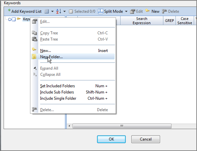
In the Tree pane, choose the folder you want to hold the keyword by highlighting it. If no folder exists, such as the case with Figure 7-30, you can simply allow your keywords to be stored in the root, or you can create one by right-clicking the root of the Keyword tree in the tree and choosing New Folder, as shown in Figure 7-31.
Figure 7-31: Creating a folder to contain and organize keywords
Now that you have a folder in which to contain your keyword, in the Tree pane, highlight this folder. Once you highlight the folder, you can launch the New Keyword dialog box in several ways:
· You can right-click in the Table pane and choose New.
· You can right-click the containing folder in the Tree pane and choose New.
· You can choose Edit > New.
· You can press Insert on the keyboard.
Regardless of the launch method, you are presented with the New Keyword dialog box shown in Figure 7-32.
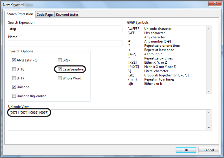
The dialog box provides numerous options or controls. We’ll begin with the Search Expression box, because it is the core component of your search. In this box, you enter your search string. At this point, you should keep your search simple. Because you are working with the case from the previous chapter, search for two keywords associated with a message about a money pickup, or so you surmise. Enter the search expression steg, as shown in Figure 7-32.
Figure 7-32: In the New Keyword dialog box, you create keywords and assign search options to go with it. By default, searches are not case sensitive, meaning EnCase searches for uppercase and lowercase hex values for your keyword, as shown in the Unicode View box.
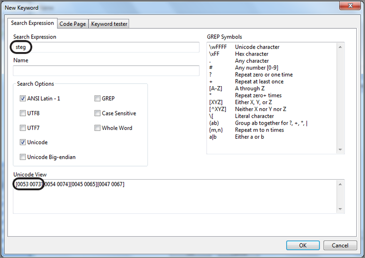
If you look in the gray box labeled Unicode View in Figure 7-32, you see the hex values for the characters you entered in brackets in both their uppercase and lowercase values. There are two hex values for each character because, by default, your search is not case sensitive and because EnCase will look for both uppercase and lowercase letters of the search expression you entered. I have circled the character(s) as it appears in uppercase and lowercase in hex. Most times, you probably should accept this default setting to find your search string in its varied renditions of all caps, no caps, or mixed caps.
Searching for both uppercase and lowercase characters increases search time compared to a case-sensitive search. If you know your search term appears in a certain format, you can select a case-sensitive search to save time and reduce the number of false positives. When you do, only the hex values for the exact characters you have entered for your search expression appear in the Unicode view, as shown in Figure 7-33. Remember from the previous section where I said that searching for an uppercase letter is different from searching for the lowercase of the same letter because they are both represented by different hex values in the ASCII table.
Figure 7-33: When making the search Case Sensitive, only the hex values for the keyword exactly as you typed it appear. Compare this to Figure 7-22, where the search was not case sensitive, and hex values for both uppercase and lowercase were present.
For purposes of this search, don’t use any other search options. You have, however, many other search options to choose from for a variety of searching needs, as described in Table 7-5.
Table 7-5: Keyword search options
|
Tab |
Name |
Description |
|
Search Expression |
Search Expression |
The actual search string or expression is typed into this field. |
|
Search Expression |
Name |
Giving your keyword a descriptive name can be helpful. This “label” appears with the keyword in the Search Hits view. Some keywords are obvious and may not need a name. But when you have complex GREP expressions, account numbers, non-English words, or the like, naming is very important. |
|
Search Expression |
Case Sensitive |
This option turns on or off the case sensitivity of your search. With it on, the search will be done exactly according to the case you specified. |
|
Search Expression |
GREP |
With this option, you can use the standard GREP input symbols and characters to create custom searches that can range from extremely focused to very broad, depending on your search needs. (See “Conducting advanced GREP searches” later in this chapter.) |
|
Search Expression |
ANSI Latin - 1 |
This specifies ANSI Latin - 1 as the default code page for the search. If you deselect it, you need to specify a code page on the Code Page tab. |
|
Search Expression |
Unicode |
Unicode, as previously discussed, uses 2 bytes (16 bits) for each character compared to 7 bits for low ASCII and 8 bits for high ASCII. If this option is off, searches will not find your expression if it appears in Unicode. When this option is on, searches will find your expression in both ASCII and Unicode formats. Unless you specifically don’t want to find your search term in Unicode, you should turn this option on if you want to conduct a thorough search. |
|
Search Expression |
Unicode big-endian |
PC-based Intel processors process data in a little-endian format, meaning the least significant bits are read first. Non-Intel processors are used in some Unix and Mac systems, and those processors work in the reverse order from the Intel. This is big endian. The most significant bits are read first. When searching for data stored in this format, select this option. Apple switched over to Intel-based processors for its Mac OS computers in 2006. It is now important to know from which system Mac OS data originated. |
|
Search Expression |
UTF-8 |
This is an encoding scheme defined by the Unicode standard in which each character is represented as a sequence of up to 4 bytes. The first byte tells how many bytes follow in the multibyte sequence. It is commonly used in on the Internet and in Web content. |
|
Search Expression |
UTF-7 |
This is an older encoding scheme that is mostly obsolete. It uses octets with the high bit clear, which are the 7-bit ASCII values. It is used for mail encoding, but it is a legacy scheme. |
|
Code Page |
Code Page |
Using the code pages in this list, EnCase can display and search for non-English languages. See Chapter 20 of the EnCase user manual. |
|
Keyword Tester |
Keyword Tester |
With this feature, you can test keywords on sample data files before running them against your case. This can save you hours of run time, particularly when you are testing new GREP expressions. When you switch to the Keyword Tester tab, your keyword carries over. Browse to the file containing your test data, and click Load. The results are displayed in the View pane in both hex and text. If you need to tweak your keyword, do so in the keyword box, and the results in the View pane are displayed in real time, making it very handy for fixing keywords. |
Managing Keyword Files and Folders
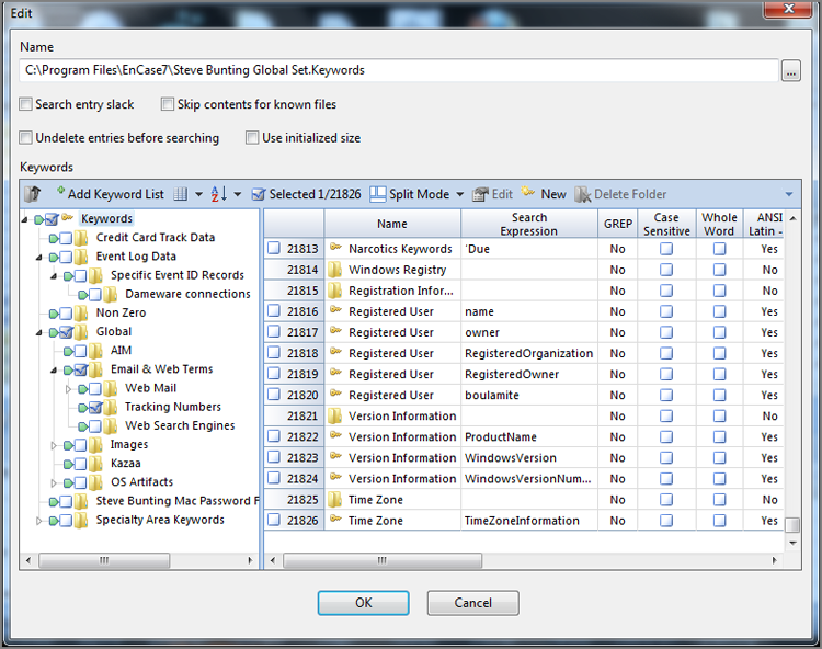
When you begin to create keywords, it is best to get organized from the beginning. You can create and store related keywords in files (with a .keyword extension) and use files to organize. Within .keyword files, you can also create folders to further organize keywords. Figure 7-34 shows how you can use folders to organize keywords. At any level that you want to create a folder, place your cursor on that level, right-click, and select New Folder. You can name the folder at the time of creation or rename it later by right-clicking or by selecting the folder and pressing F2.
![]()
Normally, you start a search by clicking Raw Search Selected Or All, but the search runs only if a keyword is selected. Once you create a keyword and run it, you can then edit the keyword file later, adding keywords, organizing, expanding, and so on. If you don’t select any keyword, the search doesn’t run and you can save it only, which becomes a handy way to organize and manage your collection of keywords that you will reuse. Also, with the Raw Search menu open, you can import keywords. For example, you can export keywords from legacy EnCase versions and import them into EnCase 7.
Figure 7-34: Keywords can be organized into folders. Right-click at the desired folder level, and choose New Folder. This set was imported from EnCase 6 and has more than 21,000 keywords.
Additionally, you can delete a folder by selecting it and pressing the Delete key or by right-clicking and choosing Delete. You can move a folder from one location to another by simply by dragging it and dropping it in the new location within the Tree pane. You can rearrange the order of folders at a given level by highlighting their parent folder in the Tree pane. The child folders will appear in the Table pane. The folders in the Table pane have “handles”—the number box at the left side of the Table view for each row or folder. You can drag the folder up or down in the order by dragging and dropping the folder row by its handle.
If you use folders to organize keywords, you can view, add, or modify those keywords by selecting that folder in the Tree pane, as shown in Figure 7-34. The same Set Included Folders trigger used in the Case view (see Chapter 6) also works here and in other views. By turning on the Set Included Folders trigger in the Tree pane, you can work with keywords from that level down in the Table pane, as shown in Figure 7-35.
Figure 7-35: The Set Included Folders trigger is turned on at the top level, placing all keywords in all folders in the Table pane.
Adding Sets of Keywords
Before you actually conduct a search, you need to consider two other methods of bringing keywords into EnCase: importing or adding keyword lists. Before you can import, you must know how to export, because importing uses a previously exported keyword list.
Importing and Exporting Keywords
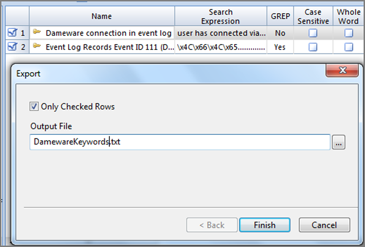
To export a keyword list, with all search properties intact, the best way is to organize the keywords into a folder. You can right-click keywords in the Table pane and drag them to a Tree pane folder. Upon releasing the mouse, you can Move or Copy them. Choose Copy. When you are done, you have the keywords you want to export in one folder. Alternatively, you can export the entire list by starting your export at the root level of the keyword list in the Tree pane. To export, in the Tree pane right-click the folder level at which you want to export, and choose Export. Figure 7-36 shows the resulting dialog box. Simply browse to a suitable location for your export file, and click OK to finish.
Figure 7-36: The Export dialog box for exporting a keyword list for importing. Browse to a suitable location, and click OK to finish.
To import an exported keyword file, choose the level or folder in the Tree pane for your import location, and right-click. Choose the Import option, and you will be prompted for the path to the import file. Once that file is located, click OK, and the entire folder structure is imported in the same tree structure it had when you exported it.
Adding Keyword Lists
Another method of adding keywords is to add keyword lists. Choose the location for your keyword list. You can select a folder in the Tree pane or add it to a folder’s list of keywords in the Table pane. Once you’ve selected the placement of your keywords, locate the Add Keyword List menu on the toolbar and click it, as shown in Figure 7-37. The Add Keyword List menu opens, as shown in Figure 7-38.
Figure 7-37: Add Keyword List button on toolbar
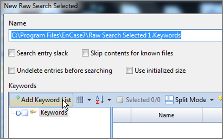
Figure 7-38: The Add Keyword List dialog box. Keywords can be typed or pasted in from other lists.
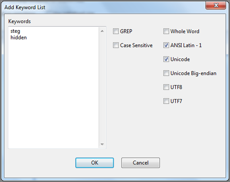
Keywords can be typed into this dialog box or pasted in after being copied from other lists. The various search options selected apply to all keywords in the list. When you have finished adding to your list, click OK, and the new keywords will be added at your selected location. If you don’t want the same options for all keywords, you can change them after they have been added as a group.
GREP Keywords
One of your keyword options in Table 7-5 was that of a GREP search. GREP is a powerful search tool derived from the Unix domain, and as explained earlier, it means “Globally search for the Regular Expression and Print.” In the various *nix operating systems, GREP is a command that recognizes a series of characters that are included in search strings, greatly adding to the versatility of string searches. EnCase embodies many of those GREP characters in its search engine, giving you pretty much the same search utility in EnCase as a search done with GREP in Unix.
The sheer power and flexibility of using GREP expressions over a regular search strings is phenomenal. Clearly, GREP expressions are tools a competent examiner must know well. It is also a topic to which considerable attention is given in the certification examination. Tests aside, GREP expressions are fun to work with and can really save you time and allow you to search for information you couldn’t find any other way.
Introduction to GREP Symbols
Table 7-6 lists the various GREP characters supported by the EnCase search engine. As you go through the list and see the examples, you’ll begin to appreciate their utility. Next, we’ll work with some examples that will help you with practical applications of GREP expressions in real-world searches.
Table 7-6: Syntax for GREP characters or symbols
|
GREP symbol |
Meaning |
|
. |
A period is a wildcard and matches any character. |
|
\255 |
This is a decimal character (period). |
|
\x |
This is a character represented by its hex value. For example, \x42 is the uppercase B. Rather than searching for B, you can search instead for \x42. |
|
? |
A question mark after a character or set means that the character or set can be present one time or not at all. An example is kills?, which finds both kill and kills. |
|
* |
An asterisk after a character matches any number of occurrences of that character, including zero. This one is similar to a question mark, but instead of one time or not at all, it means one time, not at all, or many times. An example is sam_*jones, which finds samjones, sam_jones, or sam____jones. |
|
+ |
A plus sign following a character matches any number of occurrences of that character, except for zero. Again, this one is similar to its cousins (? and *), except that the character preceding it must be there at least once. It can be present once or many times, but it must be present to match. An example is sam_+jones, which finds sam_jones or sam____jones. It does not find samjones because at least one underscore must be present. |
|
# |
A pound sign matches a numeric character, which is zero through nine (0-9). For example, #### finds 1234, 5678, or 9999, but it does not find a123 or 123b, and so on. |
|
[ABC] |
Any character in the square brackets matches one character. For example re[ea]d will find read or reed but will not find red. |
|
[^ABC] |
A circumflex preceding a string in brackets means those characters are not allowed to match one character. For example, re[^a]d finds reed but does not find read since a is not allowed to match. |
|
[A-C] |
A dash within the square brackets defines a range of characters or numbers. For example, [0-5] finds 5 but does not find 6. |
|
\ |
A backslash preceding a character means that character is a literal character and not a GREP symbol or character. For example, ##\+## finds 34+89 or 56+57 but does not find 566+57. Preceding the + with a \ tells EnCase that the + is not to be treated as a GREP character but merely as a plus sign. |
|
{X,Y} |
The character preceding a pair of numbers inside curly brackets may repeat X toY times. {2,4} would repeat two to four times. For example, a{2,4} finds aa or aaa or aaaa. It does not find a. |
|
(ab) |
Parentheses group characters for use with the symbols + (plus), * (asterisk), and | (pipe). See the next symbol for an example. |
|
a | b |
The pipe symbol acts as a logical OR, and a|b finds a or b but not c, d, and so on. To combine the previous symbol (parentheses) with this one for a more meaningful example, encase\.(com)|(net) finds encase.com and encase.net but does not find encase.org or encase.gov. |
|
\w1234 |
This allows searching for Unicode code, where 1234 is four integers for Unicode code from the Unicode chart. |
Creating Simple GREP Expressions
Now that you know the syntax for GREP, you can use a little creativity along with what you have learned thus far to create some useful GREP expressions. While you are doing it, you’ll see how GREP works, and it will become second nature after a while. As an added bonus, you’ll get to see EnCase’s Keyword Tester in action, which will prompt you to use it quite often; it is a great way to test keywords and will save you loads of time.
You’ll often be faced with finding a set of numbers, where you don’t know what the numbers are but do know the format in which they should appear. In a corporate environment, you might want to know whether employees are storing Social Security numbers in plain text on their workstations. Such a practice may violate company policy or worse (if employees are stealing the numbers). In a criminal investigation, you may want to search for Social Security numbers that a suspect may have stolen, but you won’t know the numbers. In either setting, you are looking for unknown Social Security numbers and want them all if they are present.
You know that Social Security numbers are nine digits and that sometimes those numbers are separated by spaces, such as 123 45 6789, or by dashes, such as 123-45-6789. Sometimes there are no spaces or dashes, such as 123456789. Thus, you want one GREP expression that will find nine digits stored in any of the three formats.
As the starting point, you need to find nine numeric characters, so you need #########. Next, you need to allow for separators consisting of a space or a hyphen, but you also need to allow for no separator at all. The GREP expression [ \-]? means you will allow the characters in the brackets to appear either one time or not at all. Within the brackets is a space or a literal hyphen. (Because a hyphen is also a special GREP symbol, you need to use the backslash to indicate that you’re looking for a literal hyphen, not using a symbol.) You will allow one to appear either once or not at all. If you inserted the [ \-]? between the third and fourth numeric characters and again between fifth and sixth numeric characters, you’d have the expression you need: ###[ \-]?##[ \-]?####. Note, do not include the period (.) at the end of the sentence in your GREP expression, because in GREP it means “any character.” This would be OK in most instances. However, it takes extra searching time, and if the Social Security number was at the end of a text file, it would not find the number, because there would be no character following the number.
Testing GREP Expressions
If you were to test this GREP expression, it would find each of the previous examples and in all three formats. At first glance you might be satisfied with the expression, but the moment you tested it on a real case, you would be overwhelmed by the number of false positives returned. In Figure 7-39 I used Keyword Tester in EnCase to illustrate this point. The GREP expression is inserted as the keyword, and GREP is enabled. I created a text file with three different Social Security number formats along with a string of 10 numbers. Using the Keyword Tester, I browsed to the test file and then clicked Load. The search engine looks for the keyword in the test data and returns the results.
Figure 7-39: The Keyword Tester tests a GREP expression against a small text file containing sample text to search.
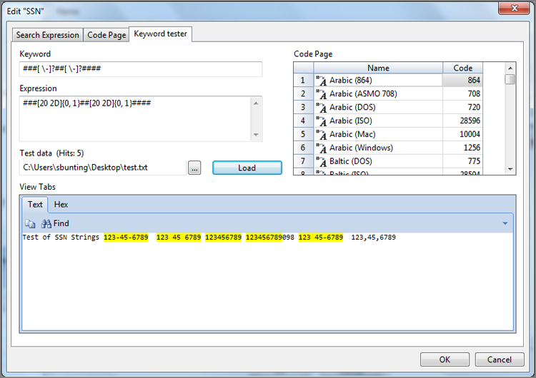
As you can see, this expression finds the occurrence of any nine numbers grouped together. The first three are SSN examples, and it finds them, but it also finds the next two. The fifth hit is an odd example of a Social Security number with a space and a dash used as breaks. Our GREP string will find this one as well. The fourth one is a string of 12 numbers. You would want nine numbers and no more. The way you have this GREP string constructed, it will find nine numbers among 10, 11, 12, 13, 14, or more numbers. Arrays of more than nine numbers are quite common, and finding them all is clearly not in your best interest. You want nine and no more.
If you were to take the expression and apply some logic and then some GREP characters, you could remedy the situation. Let’s first apply the logic.
To find nine numbers standing alone instead of nine numbers in a string of more than nine numbers, you could apply a rule of sorts to the expression. You could say that the character preceding or following nine numbers can be anything except a number. Such a condition finds nine numbers standing alone, which is what you want. You now have the logic in place.
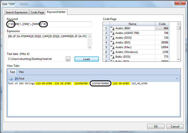
Next, you need to express the logic in a GREP expression. To create such a condition using a GREP expression, you use the square brackets and the circumflex to specify what you do not want. Thus, the expression [^#] says that the character can’t be a number. Anything else will match, but not a number. If you append this to the front and back of the string, it looks like [^#]###[ \-]?##[ \-]?####[^#]. Again, do not include the period (.) in the GREP expression. Figure 7-40 shows this revised GREP string being tested against the test data file. It finds nine-number strings in any of our Social Security number formats, but it does not find ten-number strings. It works—and you are done.
Figure 7-40: I’ve used the EnCase Keyword Tester to test the revised GREP expression. By adding to the beginning and end, it finds only nine-digit SSN strings and not strings of ten or more digits.
Sometimes you need to locate webmail addresses from one of the major ISPs that allow anonymous free accounts (such as Hotmail, Yahoo!, and Netscape). There are others for sure, but these three ISPs account for most you will encounter and are a good starting point for this example. You can modify your search as your needs dictate. You could create three separate keywords (@hotmail.com, @gmail.com, and @yahoo.net), or you could use one GREP keyword to find all three.
There is usually more than one way to create a workable GREP expression, but typically one way is cleaner or easier to work with. To solve the problem, let’s use the parentheses and pipe (logical OR) expressions. So that you find email addresses and not Uniform Resource Locators (URLs, better known as web addresses), begin with the @ symbol. Because any one of the three services can match, place each within parentheses and separate them with an OR, or pipe symbol. The expression thus starts as @(hotmail)|(gmail)|(yahoo). This means that any string beginning with the @ symbol followed by hotmail or gmail or yahoo will match and be found.
From a practical sense, you could probably stop there and find what you are seeking, but since you want to learn more about GREP, let’s continue the exercise. To find .com or .net on the end of this string, you need to add some more GREP characters. The period, or dot, is easy, but you need to make it a “literal period” because a period without the literal symbol is a wildcard character in GREP. You can represent it as \., which means a literal period.
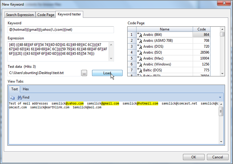
To find .com or .net, you can use the same method you used in the preceding paragraph to find the mail services: the string in parentheses separated by logical OR (pipe symbol). The final GREP expression is @(hotmail)|(gmail)|(yahoo)\.(com)|(net). When you test it, as shown in Figure 7-41, it finds the webmail services you are seeking and does not find the others, which was the intent.
Figure 7-41: I’ve used the Keyword Tester again to test the expression, which finds email addresses for any of the three webmail services I was seeking.
Tracking Numbers and Drug Runners with Brown Shorts
A mailing service had been receiving regular packages from a young man for several months. Each time he declared the contents as videotapes. One day the young man dropped off a package and promptly left after paying the fee. On this occasion he had failed to package it properly. The clerk had to repackage the parcel when he left. Instead of a videotape, as declared, the package contained a large bottle of Percocet. The clerk promptly called the police, who began an investigation.
The intended recipient of the Percocet found it in her best interest to cooperate because she happened to be an employee of a law enforcement agency in another jurisdiction. As it turned out, the young man sold a variety of painkillers via email, which was arranged by “referral” by a trusted third party. The sting was set up using the soon-to-be-former law enforcement employee, and the young man was arrested when he attempted to mail the next parcel at the mailing service counter. His pocket change at the time of his arrest was almost $10,000.
A search of his apartment revealed no details regarding his operation, and I was asked to examine the computers he used at his place of employment. It turns out he was a chemist and accessed several computers as he moved about his lab. The involved systems were imaged, and the details started to unfold.
The defendant was a member of a website that offered six levels of password-protected forums for its members. The forum topic at all levels was strictly devoted to the use of drugs, with an occasional referral for sales. Our defendant had two identities, one as a user and one as a dealer. When folks wanted to know where the user obtained his painkillers, he’d refer them to himself under his other identity. The recommendation and referral was always with the highest regard, naturally.
The operation was simple. All sales were paid using Western Union money transfers. All amounts were sent in increments that were less than $1,000 so that no identification was required to send or receive funds. A challenge question and answer was all that was required, which was all sent in an email. All used the various anonymous webmail services, especially “hushmail,” to disguise their identities. All used abbreviated and altered code words for the drugs to avoid detection by company web or email content filters. For example, “o*y” was used for oxycodone. There was quite a list, and all users of this website used it religiously in their web posts and in their emails.
All shipments were sent via United Parcel Service (UPS) because they preferred to use couriers with “brown shorts” for whatever reason. As soon as the money was received, the drugs were sent via UPS, and the defendant sent an email to his customers along with the UPS tracking number. The defendant tracked the various shipments using the UPS web-tracking service to assure delivery.
While conducting the forensics examination, it became apparent to me that UPS tracking numbers were the common link because they appeared in cached web pages and email correspondence between the defendant and his customers. If all UPS tracking numbers could be located, it would link deliveries, email addresses, quantities, payments, real names, real addresses, and dates and times.
I contacted UPS, and it provided information about the numbers and letters in its 18-character tracking number sufficient to build a GREP expression that would find all UPS tracking numbers in their various formats. With that search term in place, I located all UPS tracking numbers.
Identical tracking numbers were grouped together, and all information relating to that number and its drug sale was linked. Using this method, I identified all of his customers (more than 20 scattered around the country) by their real names and physical addresses. With this information, it was easy to build a spreadsheet that accurately depicted his sales to each customer. Because he was selling thousands of dollars worth of illegal pain killers each week, it was easy to understand why he walked around with $10,000 in cash in his pocket.
In the final analysis, it was by dumb luck that he was caught originally, but it was computer forensics alone that revealed the depth and details of his operation. It was a GREP expression that located UPS tracking numbers that greatly facilitated the latter. When the details of his operation were fully delineated, a guilty plea swiftly followed.
Useful GREP Expressions
For those who may want to use the UPS-tracking-number GREP expression (see the “Tracking Numbers and Drug Runners with Brown Shorts” sidebar) in their investigations, it is included along with a few others in Table 7-7. The publisher’s website for this book has a GREP_Expressions folder that holds a file by the same name. The GREP expressions in Table 7-7 are contained in this file so that you can copy them directly to avoid making typographical errors. One tiny error can make a huge difference in the outcome. These GREP expressions were working at press time, but any vendor or programmer can make a change that could alter the results in the future. You should test them periodically with “known data” to be sure they are current.
Table 7-7: Some useful GREP expressions
|
GREP Expression |
Description |
|
1Z[ ]?[a-z0-9][a-z0-9][a-z0-9][ ]?[a-z0-9][a-z0-9][a-z0-9][ ]?[a-z0-9]#[ ]?####[ ]?###[ ]?# |
Finds UPS tracking numbers. This number is an 18-character string, which is unique. To date, no false positive has been found. Figure 7-42 shows this GREP expression being tested in the Keyword Tester. |
|
[a-z][a-z]#########us |
Finds U.S. Postal Service Express Mail tracking numbers. |
|
value=“############”> |
Finds FedEx tracking numbers as they appear in a web form. Too many false positives occur with the raw number, so this expression finds it in a web form. It doesn’t eliminate false positives altogether, but it does reduce them tremendously. When a number is located in a web form, a second search for the specific number often turns it up in other locations. |
|
<title>(MSN )?Hotmail |
Locates web page title used by both old and new Hotmail web pages. |
|
\x2E\x20\x20\x20\x20\x20\x20\x20\x20\x20\x20.....................\x2E\x2E |
Locates “dot double dot” signature for FAT directory entries. |
|
(http)|(ftp)|(https)://[a-z#_\-]+\.[a-z#_\-\.]+ |
Finds URL addresses starting with, of course, http, ftp, or https. |
|
<!\-\- ##:##:##\-[a-z0-9][a-z0-9][a-z0-9][a-z0-9][a-z0-9][a-z0-9] \-\-> |
Locates header for AIM Plus history files. If AIM Plus is installed, these files contain IM content. When they “roll off” or are deleted, this expression finds them in unallocated clusters as well. |
Creating GREP expressions is both challenging and fun. When you create ones that can be used in future cases, be sure to place them in your Global Keywords view. The Keyword Tester is a handy utility to test GREP expressions. Without it, you pretty much have to test expressions against your case data, which is time-consuming. GREP expressions will greatly assist you with your cases, and you should take the time necessary to become adept at creating and using them.
Figure 7-42: A GREP expression that locates UPS tracking numbers is tested against a known tracking number in EnCase’s Keyword Tester.
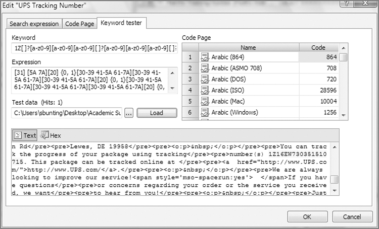
Starting a Search
Now that you have created keywords, it is time to use them to conduct searches. Before we created the keywords, we already selected the files we planned to search. In our case, we were searching all files for two users. In addition to selecting the files you want to search, you must select the search strings or keywords by which to conduct your search. By default, a keyword has a blue check mark when it is created. You can create as many as you want for any given search run and turn as many as you want on or off, but you’ll need at least one checked before a search can be run. If you reuse sets of keywords, especially larger sets, you’ll often need to select a few of many by selecting them. Once you have selected the keywords for which you want to search, you can begin your search by clicking Raw Search Select on the toolbar and clicking OK. However, there are a few search options you need to first consider. With legacy EnCase versions there was both a Keyword menu and a Search menu. Accordingly, the array of options was extensive, especially as many other processing options cluttered the Search menu. With there now being just one menu to create or edit keywords and to run the search from the same menu, the options are fewer and greatly simplified. Figure 7-43 shows the search options on the Raw Search menu, and Table 7-8 describes in detail those options.
When you conduct a raw search from the EnCase Evidence Processor, the menu is nearly the same, as shown in Figure 7-44, except that the four search options are at the bottom instead of the top. Also, the item that was dubbed “Skip contents for known files” in Figure 7-43 is dubbed “Search only slack area of known items in Hash Library” in Figure 7-44. While labeled differently, they perform the same function. You will also note in Figure 7-44 that there’s no ability to save the keywords in a file. Rather, they are saved in the evidence cache of the device to which the search is applied. After making your selections, you can start the search by clicking OK.
Figure 7-43: The New Raw Search Selected dialog box from the Raw Search menu with the various search options circled
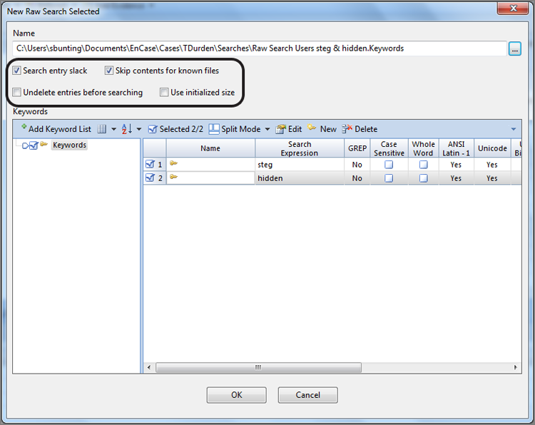
Figure 7-44: The Edit dialog box when launched from within the EnCase Evidence Processor
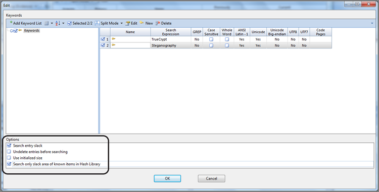
![]()
The Search Options may undergo some minor changes as EnCase 7 evolves and improves.
Table 7-8: Options in the Edit dialog box
|
Option |
Description |
|
Search Entry Slack |
If you choose this option, EnCase searches the space between the end of the logical file and the last byte of the last cluster allocated to the file. This option must be selected to find data located in FAT32 directory entries. |
|
Use Initialized Size |
EnCase will search only the initialized size on an entry, which pertains to NTFS file systems only. When an NTFS file is opened and its initialized size is smaller than its logical size, the file space after the initialized size is zeroed out. In essence, a search of initialized size searches the data a user would see in a file. |
|
Undelete Entries Before Searching |
If you choose this option, EnCase will logically “undelete” files before searching the data. This will find keywords in those rare cases where a keyword spans the starting cluster and the next unallocated cluster. The next unallocated cluster may or may not belong to the file, but for the purposes of this search, the assumption that it does belong is forced on the search criteria. |
|
Skip contents for known files or Search Only Slack Area of Files in Hash Library |
To use this option, a previous hash analysis must have been done, or one must be done in conjunction with this search. If a file exists in the hash library, regardless of category (notable or known), the logical file is not searched. This feature can save time because known files are excluded from search while their slack areas are still searched. If this feature is turned off, a file selected for search will be completely searched (both logical file and slack) even if it exists in the hash library. |
![]()
Webmail is often sought by examiners. The manner by which this has been carried out and the location of the tool have varied with various EnCase versions. Formerly webmail was parsed with an EnScript found among the Forensic EnScripts. EnCase 7 now includes this tool in the EnCase Evidence Processor as a special carve option under the File Carver. Ideally, this will save you a few steps when you need it!
Viewing Search Hits and Bookmarking Your Findings
EnCase 7 puts all search results under the Search tab, consolidating it for the first time. Past versions of EnCase had search results in different locations, depending on whether it was a raw search or indexed search. To open the Search pane, simply go to the View menu and choose Search. The Search tab contains subtabs, with one for Index, Tags, and Keyword hits. The subtab that opens is typically the last one used. Click the tab with the key icon, and the Keyword hits tab opens, as shown in Figure 7-45.
Figure 7-45: Keyword hits tab where the results of raw searches are located
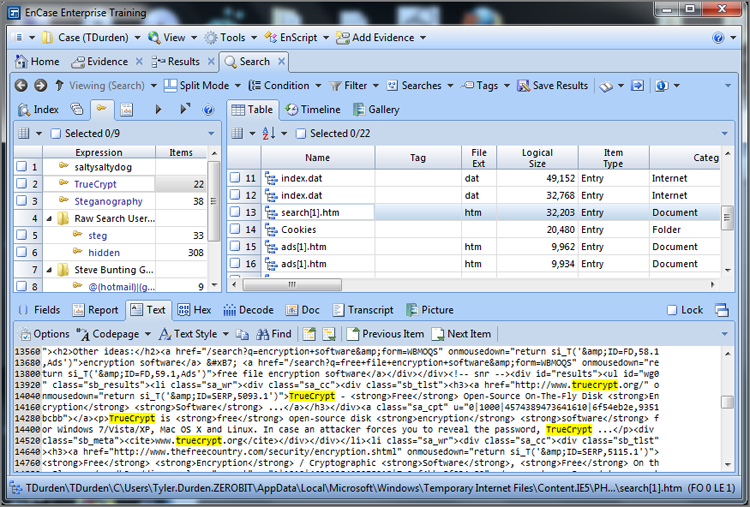
![]()
As of EnCase 7.04, a Raw Search of selected items will send the results of the search to the Results view, however those same results are also available in the Search view on a tab labeled “Keywords”.
Figure 7-45 reveals lots of information about the new keyword search hit interface. In the left pane or Tree pane, if a raw search was conducted from the Evidence toolbar, there will be a folder bearing the name of the file in which it was stored. In that folder will be the various keywords. The keywords expression column will contain the search expression unless it was given a name, in which case the given name will supersede the expression. You should get in the habit of naming keyword expressions that aren’t self-evident as to their meaning. Months can go by, and what made sense the day it was created often becomes obscure with the passage of time. You can do much analysis work directly from the Search tab. When viewing keyword search hits, some viewing options are available. The default view is the Table view, which is shown in Figure 7-45. You can view the files in which the keyword search hits appear in the Timeline and Gallery tabs or views. These are the same tabs or views you are accustomed to using in the Evidence tab, so there is not much further explanation needed.
Regardless of how you choose to group and view your search hits, you have many tools and options available from the Table pane when accessing the right-click menu. These tools and options are described in Table 7-9.
Table 7-9: Right-click menu options in Table pane of the search hits view
|
Menu name |
Description of function |
|
Copy |
Copies the data in the table field in which the cursor is placed to the clipboard, which is good for copying file names, hashes, full path, and so on. |
|
Save Results |
Saves results of search to a file. |
|
Bookmark |
Launches the window by which search hits may be bookmarked. This will be covered in detail in the next section. |
|
Go to file |
Launches an entries viewing tab within the Search tab and places the focus on the selected file in the Table view pane within the context of its path in the Tree pane to its left. |
|
Find Related |
Finds files related by filename or by time. |
Bookmarking
Bookmarks are references to specific files or data. Also, they can be notes inserted into the bookmark structure to provide additional information. Bookmarks can be created nearly anywhere that data is located, including the Search Keywords view, often called the search hits view. By having all bookmarks available in a single view—the Bookmarks view or subtab—the bookmarks can be organized into a hierarchical tree that is subsequently rendered as a report of your findings and analysis.
As previously emphasized, creating a well-written, meaningful report that also presents well is a critical skill for competent examiners to develop. Because bookmarks are the foundation of your report, bookmarking is likewise a critical skill.
Some bookmarks, such as the search summary and the case time settings, are created by EnCase as background logging functions, but most are created directly by the user. In the following sections, I’ll cover the various types of bookmarks and how to create them. I’ll also show you the basics of arranging and organizing your bookmarks, which will pave the way for the report-writing session in Appendix A.
Highlighted Data Bookmark
One of the most common bookmark types is the Highlighted Data bookmark. It is often called a sweeping bookmark or a text fragment bookmark. To create such a bookmark, you locate the data of interest in the View pane and select the text or data using a click-and-drag technique, with the starting point being the first byte in the data of interest. When the last byte is selected, release the left mouse button, and the text or data is selected and shaded or marked in dark blue. Place the cursor in the highlighted area, right-click, and choose Bookmark. Upon choosing Bookmark, you will have three options or types to choose, as shown in Figure 7-46.
Figure 7-46: A Highlighted Data, or sweeping, bookmark is created by selecting the text or data of interest, right-clicking the highlighted area, and choosing Bookmark, at which point three types are available. For a highlighted data bookmark, choose Raw Text.
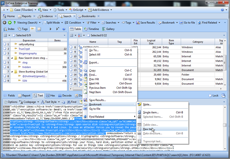
![]()
Starting with EnCase 6, in addition to the text and hex views, bookmarks can be made in the Docs and Transcripts views.
Once presented with the Bookmark Data dialog box, you can enter comments concerning the data or choose a location in the bookmark tree for your bookmark, as shown in Figures 7-47 and 7-48. Creating a comment is very straightforward. You can type a comment or paste one in if you prefer. The maximum length for a comment is 1,000 characters.
Figure 7-47: A sweeping data bookmark can be given a comment by the examiner.
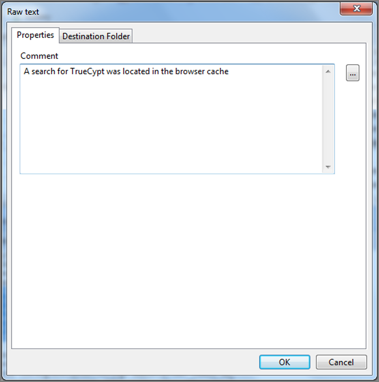
Figure 7-48: A sweeping data bookmark is placed in an appropriate folder, which in this case is an Internet artifact and from Internet Explorer.
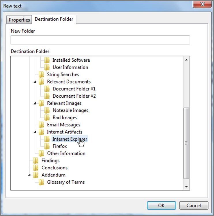
In the Destination Folder pane of the Bookmark Data dialog box, you select the folder into which the bookmark will be placed. You can also create a folder at any location you want by placing your cursor on the location and typing the folder name into the field labeled New Folder, as shown in Figure 7-49.
Figure 7-49: Creating a new folder in the bookmark destination folder tree
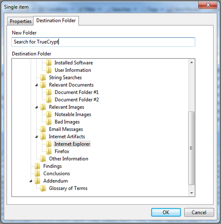
Creating folders with meaningful names and doing so in a logical outline or tree format is essential for generating good reports. The folder names act as headings and subheadings in your report outline. It is easier to add this structure as you go along when things are fresh in your mind and therefore easily and accurately labeled.
When you bookmark raw text, that is exactly how the data will appear, unless you take the added step to decode it first. What decoded means is viewing the data through one of various data-interpretive layers. It can be decoded as HTML, integers, timestamps, and so on. Figure 7-50 shows how the data we just bookmarked appears as raw text. We get to the bookmark view by simply opening the View menu on the application toolbar and selecting Bookmarks.
When we look at this data, we realize that it is HTML format as it is from a web page. EnCase can decode this data and render it into text that appears as the computer user saw it. Let’s go back to the Keyword tab under the Search tab again. With the same data highlighted in the Text tab of the View pane, and shown in Figure 7-51, simply switch to the Decode tab, located two tabs to the right of the Text tab. In the left pane of the Decode tab, you will find the various view types displayed in a tree view in five categories, which are Text, Picture, Integers, Dates, and Windows. Since our data is HTML, we will find it in the text category. Therefore, click on the text category and choose HTML from among the various text types. The data decoded as HTML will be seen in the right pane, as shown in Figure 7-52.
Figure 7-50: Data viewed as raw text
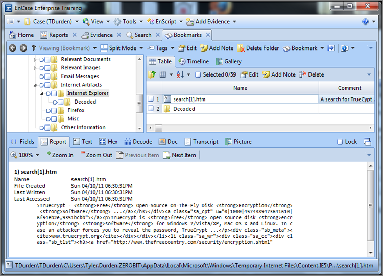
Figure 7-51: The raw text data is highlighted.
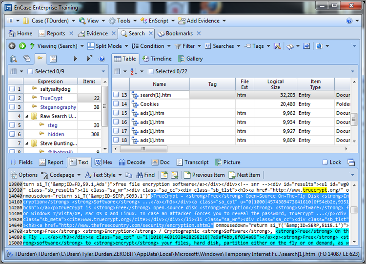
Figure 7-52: The Decode tab is used to render HTML code into text as shown in a web page.
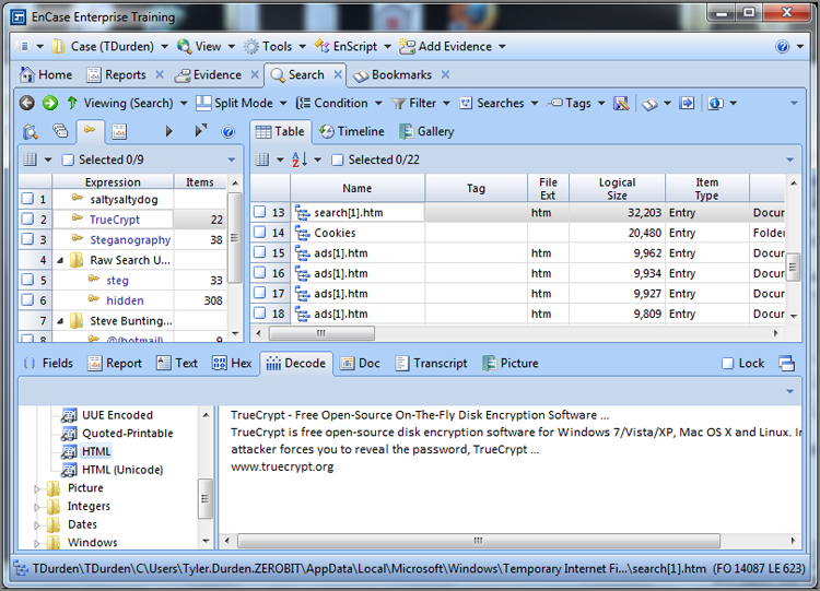
Of course, it is nice to decode and view the data, but that isn’t always that useful. You want your reader to be able to see it decoded in your report as well. To make this happen, you can also bookmark the decoded data either in addition to or instead of the raw text format. In the right pane where the decoded data appears, right-click and select Bookmark. You will be given several types from which to choose; we want to choose Data Structure for this situation. Figure 7-53 shows the menus for creating a data structure bookmark. You’ll next have the typical bookmarking options, which are Comments and Destination Folder. Once you are done, go to the Bookmarks tab and view the resulting data structure bookmark, as shown in Figure 7-54. You should note that the bookmark icon in Figure 7-53 (circled) is the same type of bookmark icon in Figure 7-54 (circled). As you see later, this decoded view will appear in the report, which is exactly what we want.
The data types from which to choose for viewing your data make bookmarking a most powerful feature. The types range from simple ASCII views to partition entries, dates, images, and various text styles for foreign languages and other special views. Table 7-10 lists the various data types along with a brief description of each type.
Figure 7-53: Bookmarking data structure of decoded data
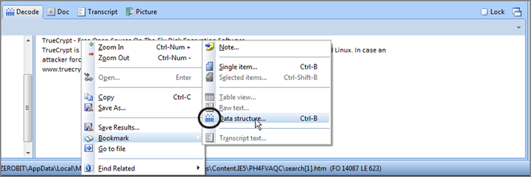
Figure 7-54: Completed data structure bookmark showing decoded data
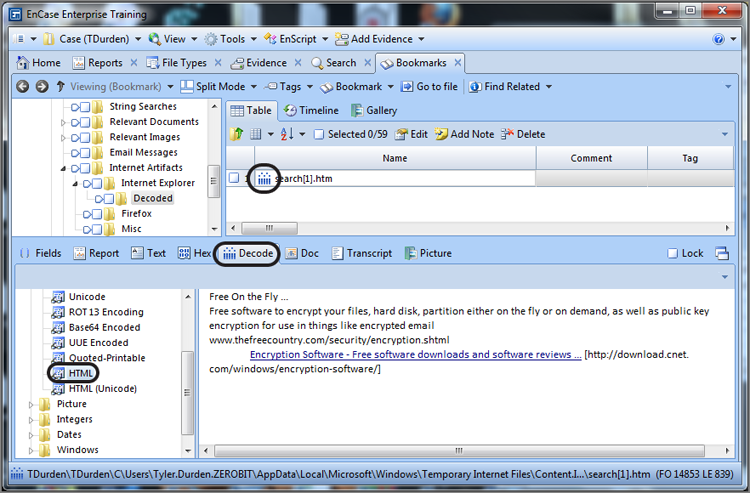
Table 7-10: Bookmark data types
|
Group |
Data type |
Description |
|
Text |
High ASCII |
High ASCII includes all characters in the full ASCII table (256 characters). |
|
Low ASCII |
Low ASCII consists of the first 128 ASCII characters only, which are mostly the alphabetic and numeric characters along with the common punctuation marks. |
|
|
Hex |
Displays values in their hexadecimal representation, a base-16 numbering system (discussed in the beginning of this chapter). |
|
|
Unicode |
Displays Unicode text in a normal format instead of “A.B.C.” as it would appear in ASCII. Unicode uses two bytes per character instead of the one-byte ASCII system. |
|
|
ROT-13 |
ROT-13 encoding is simple ASCII text rotated 13 characters so as to appear encrypted. ROT-13 makes text obscure, not secure, and is often used in newsgroups. Microsoft also uses it extensively throughout the Windows registry. Numbers and special characters do not change. Only the alphabetic characters rotate, which makes this encoding scheme easy to recognize. You will use this data type when we cover Windows OS artifacts in Chapter 9. |
|
|
Base64 Encoded |
Decodes Base64 encoded text into ASCII text. |
|
|
UUE Encoded |
Encoding scheme for mail transport. |
|
|
Quoted Printable |
An encoding scheme that uses printable ASCII characters and the equal sign to transmit 8-bit data over a 7-bit data path. |
|
|
HTML |
Renders HTML code into a text view. HTML is the language of the Web. Thus, this view is extremely useful in bookmarking web page fragments. |
|
|
HTML (Unicode) |
Unicode HTML. |
|
|
Picture |
Picture |
EnCase’s built-in viewer will display the following image types: JPG, GIF, EMF, TIFF, BMP, ART (AOL Johnson-Grace), and PSD (Adobe Photoshop). |
|
Base64 Encoded Picture |
Base64 is a type of encoding used for email attachments whereby high-bit ASCII characters are encoded using low-bit ASCII characters. This causes file sizes to grow by about 30 percent. |
|
|
Integers |
8-bit, 16-bit, 16-bit big-endian, 32-bit, 32-bit big-endian |
Displays data in an integer format in either 8-, 16-, or 32-bit arrays. If big-endian, the most significant bit is stored and read first. |
|
Dates |
DOS |
Packed 16-bit value used by DOS to store month, day, year, and time. |
|
DOS Date (GMT) |
Displays data as a DOS date and converts to GMT. |
|
|
Unix Date |
The number of seconds that have lapsed since “epoch,” which is January 1, 1970, at 00:00 GMT (32-bit hexadecimal value). |
|
|
Unix Date big-endian |
Same as previous, except in big-endian. |
|
|
Unix Text Date |
The same base reference as Unix Date, except that the number of seconds since epoch is a 10-digit number instead of a 32-bit hexadecimal value. |
|
|
HFS Date |
Macintosh file system numeric value representing month, day, year, and time. |
|
|
HFS Plus Date |
Macintosh file system numeric value representing month, day, year, and time. |
|
|
Windows Date/Time |
64-bit hexadecimal value for Windows date/time. |
|
|
Windows Date/Time (Local) |
Same as Windows Date/Time, but for decoding 64-bit time stamps when expressed in local time. |
|
|
OLE Time |
Resolves OLE container time stamp. |
|
|
Lotus Date |
Date value for Lotus Notes database file. |
|
|
Windows |
Partition Entry |
Interprets 64-byte partition table values. |
|
DOS Directory Entry |
Interprets 32-byte DOS directory entries. |
|
|
Windows 95 Info File Record |
Interprets data from Windows 9x INFO files, which are the Recycle Bin database files. |
|
|
Windows 2000 Info File Record |
Interprets data from Windows 2000, XP, and 2003 INFO2 files, which are Recycle Bin database files. |
|
|
GUID |
Resolves and displays strings that conform to the Windows Globally Unique Identifier (GUID) format. |
|
|
UUID |
Universally unique identifier resolver. |
|
|
SID |
Resolves and displays strings in the Security Identifier (SID) format. |
After you have entered your comment and selected a destination folder, click OK. If you want to have your data decoded, you can display it in the Decode tab and bookmark its data structure, thereby rendering the decoded view in the Bookmarks section. You may want to preview each bookmark as it is created to make sure you created what you intended, and that you placed it correctly in the intended location. It is a good practice to save after each bookmark. It takes only a second or two to press Ctrl+S. The practice creates a good habit that can translate into saved data and work when bad things happen to good people, good software, and good computers.
Notes Bookmark
A notes bookmark is versatile and can hold notes, comments, or any text format you can paste into it. It enhances or further explains information in your report. The limit is 1,000 characters, and there is a built-in formatting tool for changing font size, bolding, italicizing, and setting indentations.
To create a notes bookmark, right-click at the location where you want to insert the bookmark (or within the Tree pane, Table pane, or Bookmark Data dialog box in the Destination Folder pane), and choose Add Note. Alternatively, pressing the Insert key gives the same result.
Once you are viewing the Add Note Bookmark dialog box, as shown in Figure 7-55, you can type or paste in your text. The formatting options are straightforward. The check box labeled Show in Report is selected by default. This means your notes bookmark will appear in the Report view, which is typically the result you desire. The note will be appended to the end of the bookmarks in the selected folder as somewhat of an “end note.” If you prefer it at the top, or anywhere else, you can go to the Table pane and click and drag it by its handle to the desired location.
Figure 7-55: Add Note Bookmark dialog box in which text can be typed or pasted. Limited formatting options are also available.
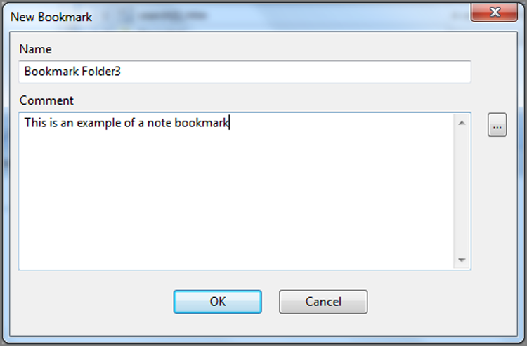
Notable File Bookmark
A notable file bookmark inserts a bookmark or reference to a file that contains information significant to your case. When you create a highlighted data bookmark, the data is shown in the bookmark and report. When you create a notable file bookmark, the data is not bookmarked. The bookmark contains the attributes or properties of the file.
To create a notable file bookmark, right-click the file from the Table view of the Entries view from the Evidence tab. Choose the Bookmark > Single Item option, as shown in Figure 7-56, and you will be presented with the dialog box shown in Figures 7-57 and 7-58.
Figure 7-56: Bookmarking a single item
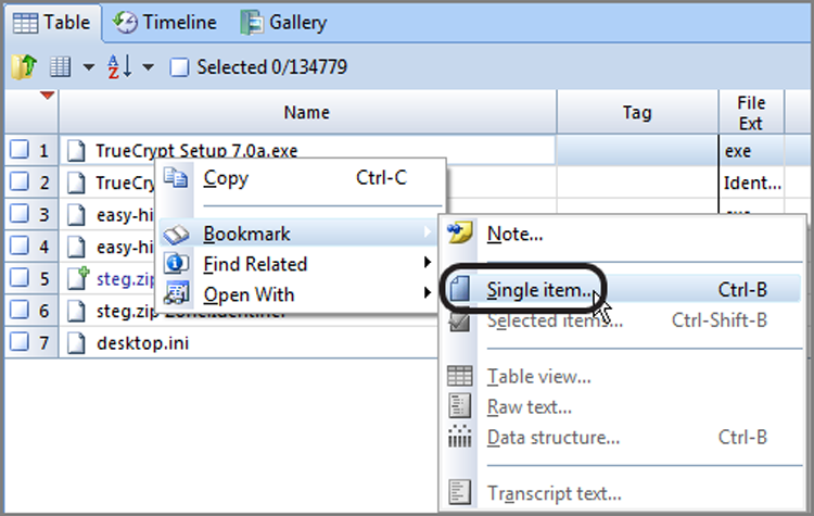
Figure 7-57: Bookmark Single Item dialog box from which you can add comments
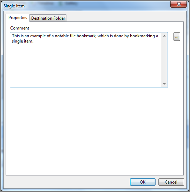
Figure 7-58: Bookmark Single Item dialog box from which you choose the Destination Folder and from which you can also create a New Folder
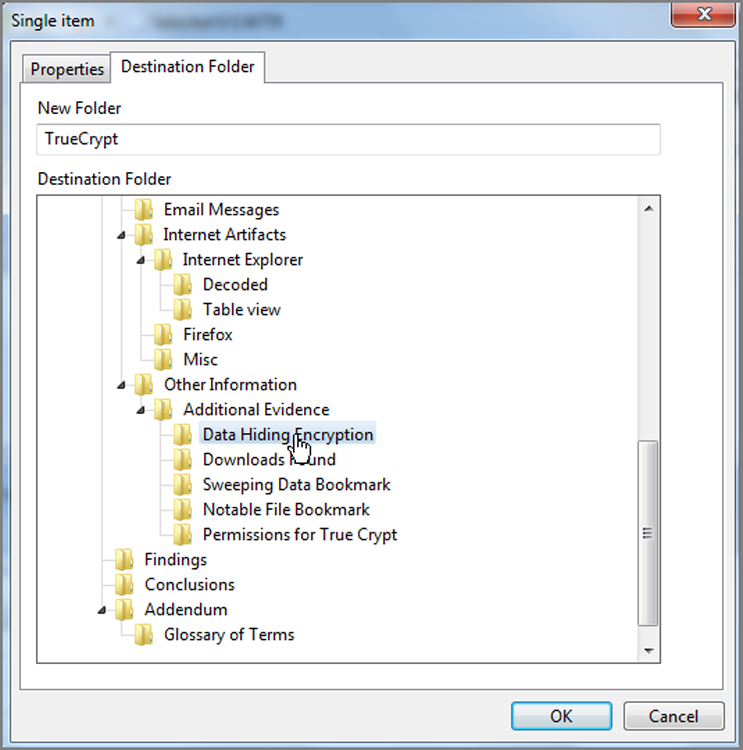
The choices are relatively simple. You choose a Destination Folder; once again, creating well-named folders is important. You can create a folder within the destination folder by simply providing the name of the folder. You can add a Comment specific to this bookmark if you want. Figure 7-59 shows the Report view created by this bookmark.
Figure 7-59: This is the Report view of notable file bookmark in the Bookmarks tab.
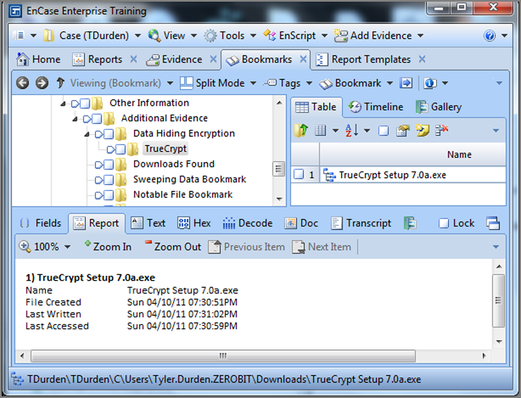
In past versions of EnCase, the metadata shown in Figure 7-59 was what appeared in your report. You could change it by editing the parent folder properties in the Tree pane and thereby customize the metadata fields that would appear in the report. EnCase 7 introduces a new way of reporting, which is greatly improved but does come with a learning curve. We’ll explore some of those features later in this chapter.
Bookmarking Selected Items
Notable file bookmarks can be created from selected items. To do so, simply select the items you want to bookmark as a group with blue checks. When you right-click and choose Bookmark, you now have the option to choose Selected Items, as shown in Figure 7-60. Next, you select a destination folder as you did for a single notable file bookmark. It is a good practice to have a folder for each group of related files. You can let the folder name describe the contents of the group of bookmarks. Additionally, you can always create a notes bookmark to further describe bookmarked findings.
![]()
Before you begin creating file group bookmarks, get in the practice of checking the Dixon check box to make sure it is deselected. It wouldn’t be the first time an examiner created thousands of file group bookmarks when they intended to create only a few! Also, you can create a single item notable-file bookmark using the shortcut keys Ctrl+B and selected items notable-file bookmarks with Ctrl+Shift+B.
Figure 7-60: Bookmarking a group of selected files
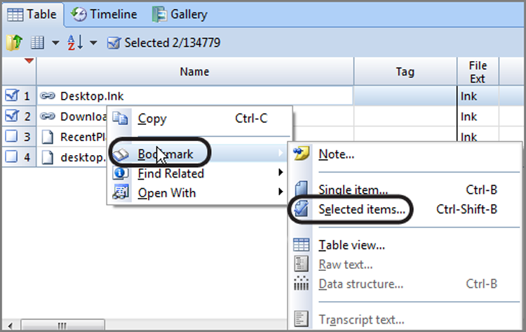
Other Bookmarks
When running various analysis routines, threads, or EnScripts, the results are often displayed with an option to bookmark the results. If the option is selected, the results are automatically pasted into a notes bookmark that is sent to the Bookmark view. Notes bookmarks are very versatile. You can click and drag the resulting bookmark to a folder of your choice for inclusion in your report. You can copy and paste data from third-party tools, Internet research, or most text data into a notes bookmark and thereby include it in your findings.
EnCase also uses another type of bookmark that is called a log record bookmark. It is most often encountered when an EnScript runs and parses data from entries. The data is written to a log record bookmark, and there is no pointer to the data. This is important when parsing the registry. Without this type of bookmark, a pointer would have to be used, and that would require leaving the registry hive files mounted, greatly increasing the case loading time.
To view log records, go to the View menu on the application toolbar and click Log Records. The log records will open in their own tab. Figure 7-61 shows the log records in a case. In this example, you will note that file verification has been run three times. The report view for the device doesn’t show this at all, only that it has been run and verified but doesn’t say when. Because we want to follow best practices and document that we verified the integrity of the acquired evidence both after acquisition and then again at the end, after all the processing is done, to demonstrate that the data was not changed or corrupted in the process, we can do so by bookmarking log records and including them in our final report.
Figure 7-61: Log records being viewed
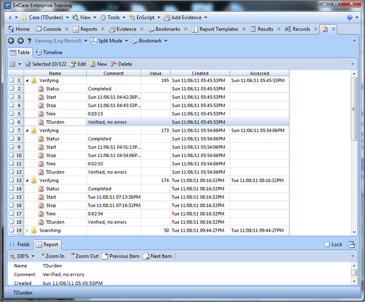
To bookmark a record log, a Table view bookmark is used, which is a new bookmark type released with EnCase 7. The Table view bookmark has many uses and is very versatile. Let’s bookmark our file integrity verifications. In our example, Figure 7-61, I want to verify my first and last verifications. I am therefore going to place blue check marks for each of the table entries associated with these two verifications, as shown in Figure 7-62. You should note that a Table View bookmark is, by definition, one that will bookmark Table view entries and that to do so, we must have at least one such entry selected before this option is an available bookmark.
Figure 7-62: Entries selected in Log Record view
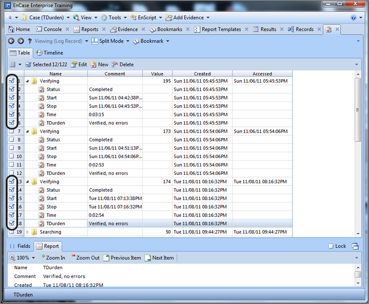
With entries in the table view selected, right-click and choose Bookmark > Table View, as shown in Figure 7-63. In the screen that follows, you give it a Name and optionally include any comments, as shown in Figure 7-64. When you click Next, you are prompted for a destination folder within your bookmark folder structure, which is in turn linked to your report layout but may not be depending on your configurations in your report template. If a bookmark is not showing in your report, the problem can almost always be resolved in the report template settings. We’ll get into that later, but it can be an issue and is worth mentioning now. In addition to selecting a Destination Folder, you can also add a New Folder, as shown in Figure 7-65. After a destination folder is selected, the final step in creating the bookmark is choosing which columns in the table view to appear in the bookmark. In this case, we’ll select all of the columns, as shown in Figure 7-66. Select Finish and the Table view bookmark is complete and may viewed in the Bookmark tab, as shown in Figure 7-67. My report template is configured such that this table will appear in my report and will appear as shown in Figure 7-67.
Figure 7-63: Bookmarking a Table view
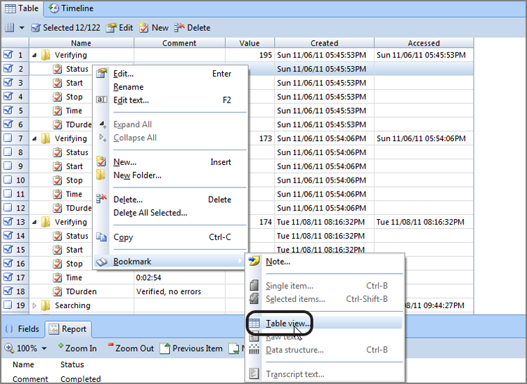
Figure 7-64: Naming the bookmark and adding comments
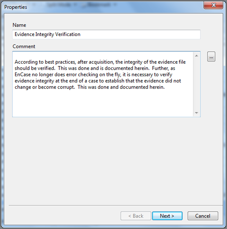
Figure 7-65: Selecting a Destination Folder and creating a New Folder
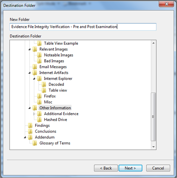
Figure 7-66: Selecting which Columns in Table view will appear in bookmark
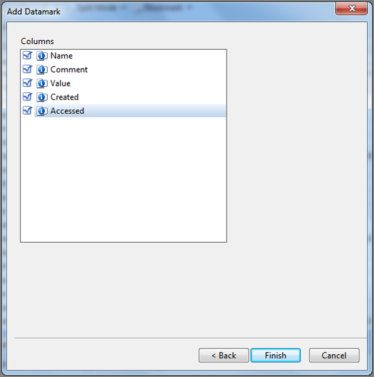
Figure 7-67: Completed Table view bookmark in Bookmarks tab
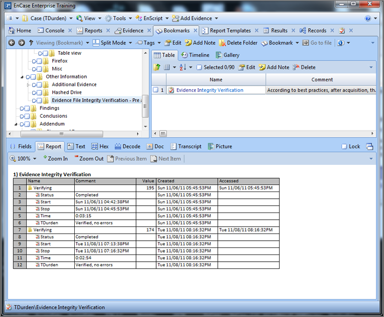
![]()
When you add a new destination folder, make sure to place it in a destination folder for which the “recursive” feature has been enabled in the report template. If not, your new folder and bookmark will not be visible in the report. This is not just for Table view bookmarks but for any bookmark type for which you choose to create a new folder. We’ll cover this feature when we discuss reports and the report template.
![]()
I’ve stated already that the Table view bookmark is very versatile. Many veteran EnCase users have no doubt seen entries in the Table view for deleted files that were overwritten. When such an entry is found and one attempts to create a notable file bookmark showing the entry for the deleted file, what you get is a bookmark for the file that overwrote the deleted entry and not the data in the Table view that you wanted to bookmark. It was out of the need to bookmark such entries that the new Table view entry bookmark was created. Now when you see a deleted file that is overwritten, you can easily bookmark that data with the Table view bookmark. Anything that appears in EnCase in a Table view can be bookmarked with this feature.
EnCase 7 tends toward fewer bookmark notes for various EnScripts and processing routines and instead sends output to log records and to the console. Veteran EnCase users who are used to finding bookmark notes for such things as hashing drives, searching, and the like will need to look to log records for the results. If you want a bookmark of such data, you now know how to create it with a Table view bookmark. In addition, output is often sent to the console. Figure 7-68 shows the output of hashing the device. You can copy the results in the Console tab and paste them elsewhere, such as a notes bookmark.
Figure 7-68: Console tab showing results of various processing tasks, with the last one being hashing of the device, which is highlighted
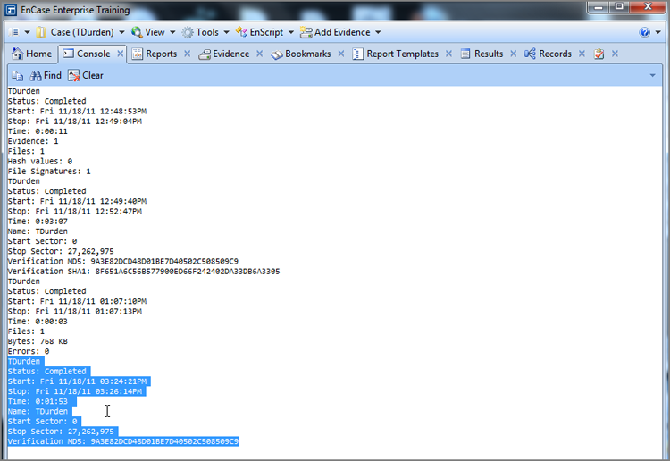
![]()
Some EnScripts will write their results to the console as part of their output. You should be cautious of this approach because anything already in the console can be overwritten. At best, anything written to the console will persist only until EnCase closes or the case is closed.
Organizing Bookmarks and Creating Reports
From the Table view pane and the Tree view pane, you have the ability to organize your findings. In the Tree view pane, you can add, delete, and move folders around. You can change the order of any folder’s contents by selecting the container or parent folder in the Tree view pane, forcing its contents into the Table view pane. From the Table view pane, any item can be moved by clicking and dragging its handle. You can drag an item in the Table view pane to another folder in the Tree view pane by the same click-and-drag method. Right-clicking and dragging provides even more in the way of granular Copy Here, Move Here, Move Selected Items Here, or Copy Selected Items Here menu options, as shown in Figure 7-69.
Figure 7-69: Right-click, drag, and drop options
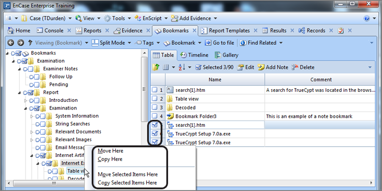
Bookmarks in the Table view have many right-click menu options. Probably the most used of these are the Delete, Delete Selected, Add Note, and Go To File options. Just remember that when you delete a bookmark, it is deleted.
Bookmark creation and organization combine to form the substance and layout of your report and thus become very critical to your final output. It pays to understand and modify the various elements because how your report appears reflects on your reputation as an examiner. For most of us, that should serve as sufficient motivation to roll up our sleeves and really understand bookmarks and how they link to reports.
In previous versions of EnCase, the Table pane included a Report tab from which the report was generated. You could preview it and eventually export it from that tab. EnCase 7 has done away with the Report tab on the Bookmarks tab. Rather, Reports has its own tab, and the configuration options for that report are done in the Report Templates tab.
As we have been creating bookmarks in this discussion, those bookmarks have been placed in the bookmark tree that was determined by the template we chose when we created our case. As I created the case with the forensic template, that template dictates the initial bookmarks and associated report template. You can create other templates or customize this one to suit your needs. As it stands, I can create a report, or at least a limited report, based on the bookmarks thus far created. To view this report, simply go to the application toolbar and choose View > Reports. The Reports tab will open, and in it you will see the report as it currently stands with your various bookmarks there. Figure 7-70 shows the Reports tab and the default report heading.
Figure 7-70: Reports tab and default report header

At this point, to export it for further editing and enhancement, merely right-click anywhere in the body of the report and choose Save As, as shown in Figure 7-71. You will next be presented with a variety of file formats that can be used to save the file, as shown in Figure 7-72. Additionally, you need to create a path and filename by which to save your report. A useful option, depicted in Figure 7-72, is the Open File check box. When checked, the saved report will open in the native application that is designated to open the saved file type. As HTML was selected, this report will open with the default browser, as shown in Figure 7-73.
Figure 7-71: Right-click in the report body and choose Save As.
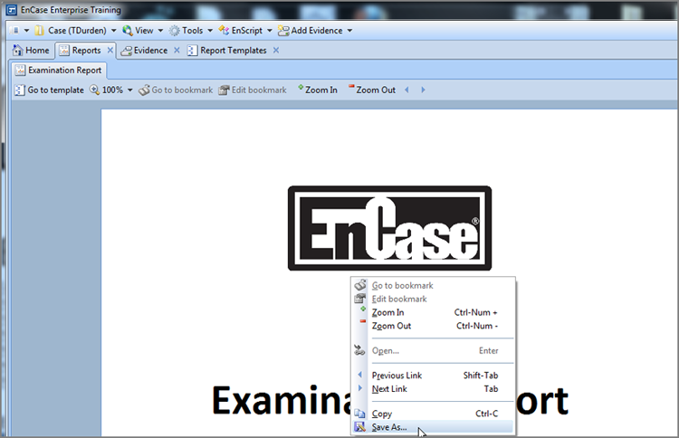
Figure 7-72: Different file format options for saving report, along with filename and path options
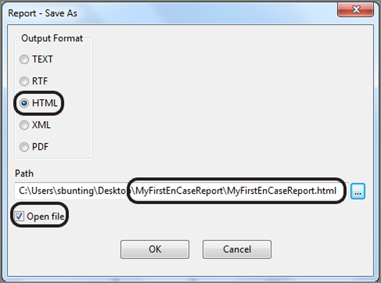
Figure 7-73: If the Open File option is selected, the report opens in the native application.
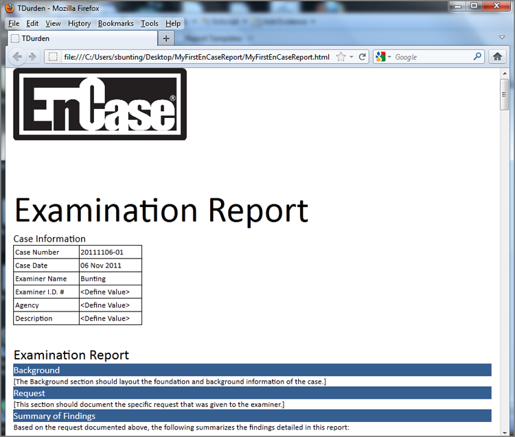
We could end our discussion of reports here, but that wouldn’t do justice to the features found in the Report Templates tab. From the Report Templates tab, you can format the report, add sections, link bookmark folders to report sections, and much more. Finally, when you have a template that is customized to your agency or company, you can save your work as a template. Then, each time you create a new case, you use this template instead of the default set. When you do, you will have everything set up for you the way you customized it.
Before starting, I suggest you create a new case with the forensic template, or one that closely suits your needs. Once open, immediately go to the Bookmark tab. In the Tree pane, under Bookmarks, drill down to Examination\Report\Examination\Other Information. At that level (Other Information), create a new folder named Additional Evidence, as shown in Figure 7-74.
If you were to now go to the Reports tab and scroll down the report, you would find that your new folder does not appear under the section Other Information, as you might expect. Figure 7-75 shows this section and the absence of your newly created folder.
Figure 7-74: Create a new folder under Other Information.
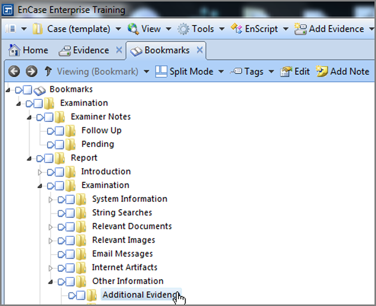
Figure 7-75: The Reports tab does not yet show your new folder.
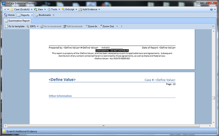
Your new folder does not yet show in the report because no link has been created between your bookmark and your report. This is a concept or feature that is new with EnCase 7. You create links between bookmarks and the report through the interface on the Report Templates tab. You can access the template from the View menu on the Application toolbar; or, if you have the Reports tab open, there is a Go To Template tool button on the Report menu bar, as shown in Figure 7-76.
Figure 7-76: Go To Template button
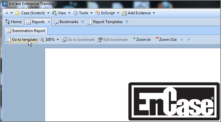
The Report Templates tab should open in the Traeble mode by default. If it doesn’t, you may want to switch to it, because it seems the better choice for working in this tab. Next, locate the Other Information section, which is in the report body and is shown in Figure 7-77. To help you see the changes you will be making, it is suggested that you switch to the Report tab in the lower View pane, also shown in Figure 7-77.
Figure 7-77: Other Information section selected and viewed in the Report tab
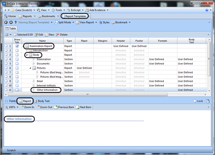
The next step is to edit the section Other Information, which is done by simply double-clicking that item. You can also right-click it and choose Edit. When you do so, you will see the Edit “Other Information” dialog box, with three tabs, as shown in Figure 7-78. It will open to the Options tab, but we want to do our work on the Body Text tab, so switch to that tab, which is shown in Figure 7-79.
Figure 7-78: Edit “Other Information” dialog box, showing Options tab
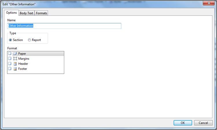
Figure 7-79: Edit “Other Information” dialog box showing Body Text tab
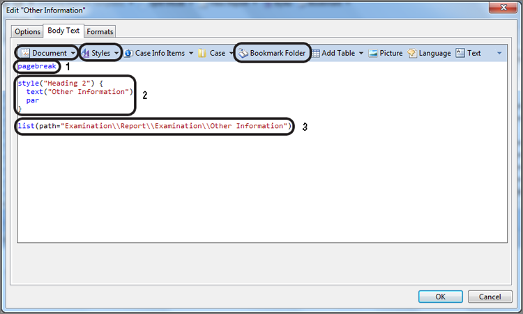
Before we start changing things, let’s get an understanding of the information we see in the body text. I have circled the three separate items in Figure 7-79 that currently exist so we can isolate and understand them. Number 1 (pagebreak) does nothing more than force a new page for this item and is generated from choosing it from the document menu, which is also circled and is immediately above it in this case. Item 2 defines a text style for the text Other Information on the report page. It is generated by choosing it from the Styles drop-down menu, which is also circled. Once inserted, the cursor will appear where you start typing text.
Item 3 is the link to the bookmark. Without this link, nothing placed in the Other Information bookmark folder would appear in the report. All that would show would be the words “Other Information.” Right now, it does not contain the recursive option, and therefore no folders placed therein show in the report, which is precisely why our folder doesn’t show. It would, however, show any bookmark placed in the root of the folder Other Information but not subfolders or the contents of any subfolders. There are two ways of fixing this: One is to add the recursive option to the existing link, and the other is to create a link for our folder and make it recursive so that all folders placed therein will appear without having to edit the template. So that we can see the difference between the two links when we are done, we are going to use the second option, which is to insert a link to our new folder and make it recursive.
Place your cursor in the whitespace under item 3 in the body text, because this will cause the next item to be inserted at this point. Next, click the Bookmark Folder menu, which will provide a listing of bookmark folders that are available to link to the report, which is shown in Figure 7-80. Select the new folder that we just created, which is Additional Evidence. Before clicking OK to create the linkage, note the two options in the upper left. I have circled them to draw your attention to them. By default, they are not enabled. Show Folders causing the name of the folder (in our case Additional Evidence) to show or not show as a header or subtitle in the report. I prefer to have it show and name my folders accordingly. Recursive causes any folders and their subfolders to appear in the report. This option was not selected for the parent folder Other Information and is the reason our new folder does not appear in the report. Again, I prefer all folders to appear in the report, which is why I create them in the first place. So, enable both of these options, and then click OK to complete the link.
Once you click OK, you are returned to the body text, as shown in Figure 7-81. You can see the link to the new folder with the two options included, which are SHOWFOLDERS and RECURSIVE. You should immediately see that the link to the parent folder did not include these options. If it contained the recursive option, what we are doing now would not have been necessary.
Figure 7-80: Menu to link bookmarks to show in report
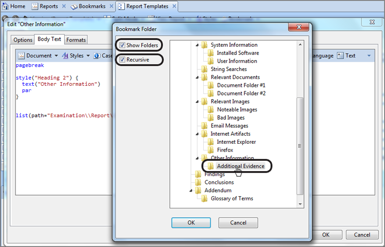
Figure 7-81: New bookmark link inserted with Recursive and Show Folders options in place
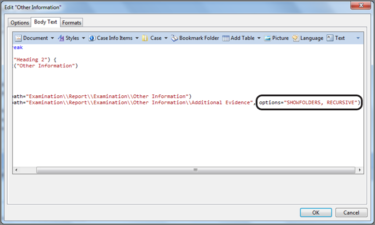
From the Edit “Other Information” dialog box, click OK to finish the work and apply it to the template. In the Report tab at the bottom, you will see the changes immediately as the newly created folder now appears in the report, as shown in Figure 7-82. You can, if you like, add a bookmark to this new folder and then check the report to make sure it appears.
Figure 7-82: New folder now appearing in report
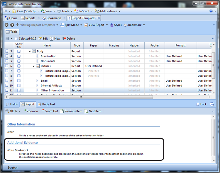
While we are working in the report template, there’s another editing option that you should be able to do, which is modify the metadata that is shown in the report. The default is to show a file’s name and MAC times (modified, accessed, and created). For some the default is sufficient, and for others it’s just the opposite. I happen to fall into the latter category, so let’s discuss how we change these settings. I have created a notable file bookmark in the new folder that we just created. If I view the report to see how this bookmark appears, I see it in the new folder (Additional Evidence), and I see the default metadata fields (name and MAC times), as shown in Figure 7-83.
Figure 7-83: Notable file bookmark with default metadata (name and MAC times)
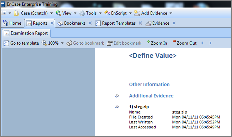
To change how metadata appears, we have to use the report template editor to edit the section where the bookmark appears. To fix this particular one, go the Report Templates tab and edit the section named Other Information, just as we did to link the bookmark to the report. This time, when the Edit “Other Information” dialog box opens, we are going to switch to the Formats tab, as shown in Figure 7-84. Among other objects that can be formatted, you will find formatting options for the various bookmark types. Our bookmark is a notable file bookmark, and you simply double-click that object to edit it. Figure 7-85 shows the open editor and the default code. I have circled the code that defines the metadata for clarity. This is the code that we need to edit.
Figure 7-84: Edit “Other Information” dialog box Formats tab
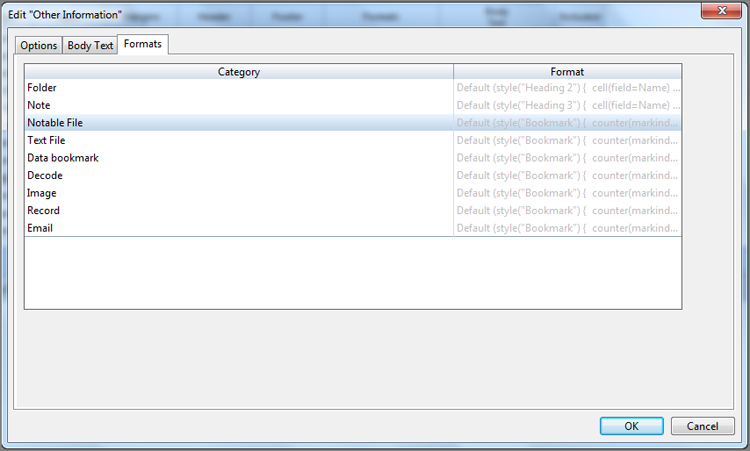
Figure 7-85: Code pertaining to metadata is circled
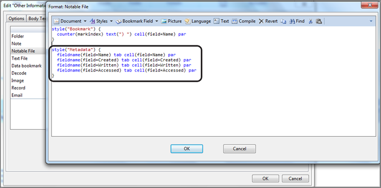
The field names that we’ll be inserting will be generated from the Bookmark Field menu. In our example, I want to insert the full path immediately following the name field. First, we have to place our cursor at the insertion point. That also means we have to insert a carriage return to achieve the proper insertion point, as shown in Figure 7-86.
Figure 7-86: Insertion point for inserting a field following the Name field
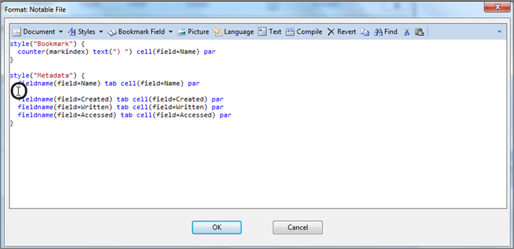
With our cursor at the insertion point, click the Bookmark Field drop-down menu and choose Item Path, as shown in Figure 7-87. The end result is the insertion of that field into the code at the insertion point, as shown in Figure 7-88. The insertion places a carriage return at the end of the code, but not the beginning, such that you could continue inserting addition fields if you’d like. What the field insertion process fails to do, and understandably so, is to place the code at the end that triggers, effectively, a carriage return; this is the par code, which is the abbreviation for paragraph. Thus, you must manually insert the par at the end of the inserted field code. To tidy things up further, I removed the carriage return, although it would not appear as such in the report. Figure 7-89 shows how the finished insertion should appear.
Figure 7-87: Inserting Item Path from Bookmark Field drop-down menu
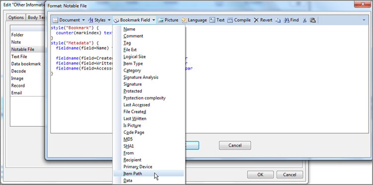
Figure 7-88: Line of code inserted without par at end and with extra carriage return
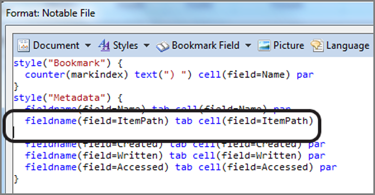
Figure 7-89: Shows finished insertion of code, which is how it should appear when done
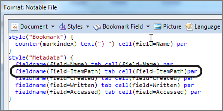
At this point, you have successfully inserted a line of code necessary to modify the file metadata that involves a notable file bookmark in this section (Other Information) of your report. Click OK in the Format: Notable File window, and click OK in the Edit Other Information window. When you do, you should see the changes appear on the Report tab for the Other Information section, as shown in Figure 7-90.
Figure 7-90: Report tab view showing Item Path field added to bookmark metadata
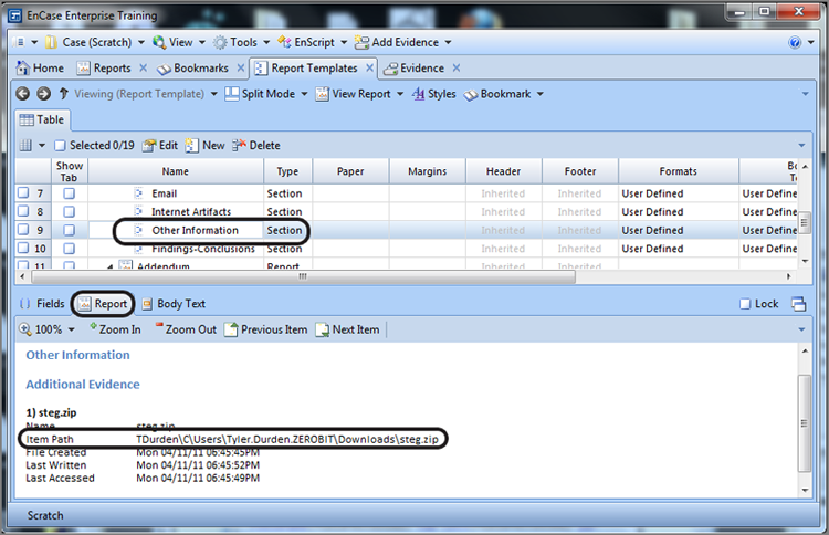
If you were reading carefully, you noted that I said that we added this field to the Notable Files bookmark for this section only. We did not insert this field for other bookmark types or in other sections. You could make changes at parent levels and have the changes inherited to the children, or you could make the changes at lower levels as preferred. Regardless of which you decide, make gradual changes and test the desired result with data as you go.
While this may seem a lot of work, once you get the hang of it, you can create the metadata fields to your liking for one bookmark type in one section and then copy and paste the code to other bookmark types and in other sections. There is more good news in that you need to do this only once, because you’ll save your work in a template and reuse it hundreds of times. Thus, it is worth the one-time effort to develop a customized template that reflects favorably upon your work. Let’s save our template and show you how to reuse it.
Let’s assume you’ve changed the metadata for your various bookmark types in the different sections according to your preferences or those of your lab. You can and should make other changes, such as the logo, lab name, and address on the title page, as well as the examination tools. The latter (examination tools) are not changed in the template but rather in the bookmarks themselves. You’ll find them appearing as notes bookmarks under the bookmark folder Examination Tools.
When all changes are completed, you simply go to the application toolbar and choose Save As Template on the Case drop-down menu, as shown in Figure 7-91. In the resulting dialog box, name your template something meaningful and clear. As shown in Figure 7-92, there are other options that can be saved in the template. The first two are paths to the evidence cache and the hash library. For now, we won’t select them. The third option, circled in Figure 7-92, is what we want to select. By saving bookmark notes, we are saving the changes we made to items such as the Examination Tools notes bookmarks that we just took the time to modify from their default data. When done, click OK to save.
Figure 7-91: Save As Template option
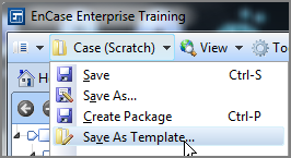
Figure 7-92: Save As Template dialog box by which to name the template and save your bookmark notes
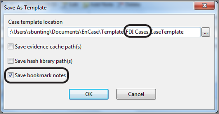
To see the fruits of your labor, create a new case, and you will see the name of the template you just created in the list of templates. Choose that template, and note that information appears in the Case Info section, as shown in Figure 7-93. You can give your case a name and click OK. You can go to your Report tab and see some of the changes made right away. Figure 7-94 shows the title page as customized. It had to be done only once and now appears with each new case. As you add bookmarks, all the customization you made will appear. From time to time you’ll make added changes and tweak your template, making it look better and more professional each time.
Figure 7-93: New Case Options dialog box with the saved template appearing in left pane
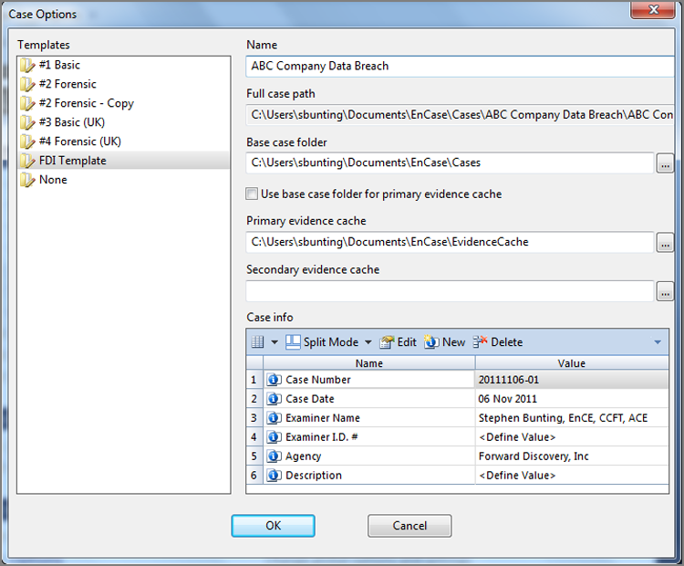
EnCase’s bookmarks and the resultant reports, to which they are linked, are very powerful and very flexible features. The addition of the report template editor makes them even more customizable. The report template, at first glance, is intimidating, but once you roll up your sleeves and make a few changes, you get used to its function and features very quickly. In a very short time, you’ll be an EnCase report power user!
Figure 7-94: A custom report is now available from the saved template and will be available for all cases going forward.

Examiners are encouraged to take the time to work with each of the features. In this manner, you can learn to quickly and easily create bookmarks that will be used to generate professional reports that convey your hard work and findings in a clear and meaningful way. In Appendix A, I will cover extensively how to work with your bookmarks to generate such reports.
Exercise 7.1
Searching for Data and Bookmarking the Results
In this exercise, you’ll import keywords and conduct a GREP keyword search of your case for data, matching your keyword. When the word is found, you’ll examine the search results, bookmarking the results using various data views. To complete the process, you’ll create a paperless report, showing the results of your work. Let’s get started.
1. Open EnCase, and from the Home tab, create a new case. Use your custom template or the forensic template. Name your case OnlineDrugSales. Accept the other defaults, and click OK.
2. From the publisher’s website for this book, download the file DefFrostyUSB16MB_TD01.E01. Go to the folder created for this case (\Users\UserName\Documents\EnCase\Cases\OnlineDrugSales). In the root of this folder, create a folder named Evidence, and place this evidence file in that folder.
3. From the EnCase Home tab, select Add Evidence and choose Add Evidence File. Browse to the evidence file just added to this case, and click OK.
4. Let’s follow best practices and check to make certain the evidence file is verified. From the Evidence tab (now open), select the evidence file in the Table pane. In the View pane, at the bottom, switch to the Report tab. Scroll down and check that the evidence file verified with no errors.
5. From the publisher’s website for this book, download the file Keywords_For_Import.txt and place it somewhere convenient, which is most likely your desktop.
6. From the Evidence tab, double-click the evidence file to have it parsed and mounted in the Entries view.
7. In the Tree pane, place a blue check mark at the device level and note the Dixon box. It should say 526/526 selected.
8. On the Evidence toolbar, click Raw Search Selected and choose New Raw Search Selected. In the right-side menu (the super-secret menu), choose Import > Open. Browse to the file we just downloaded, wherever you save it, and click OK.
9. You should have several GREP expressions in the resulting window, which are the ones mentioned earlier in this chapter. Browse to the keyword in the Tracking Numbers folder, and place a blue check mark for UPS Tracking Number. Browse to the Windows Artifacts folder, and place a blue check mark for the “dot double dot” directory. You should have selected two keywords for your search.
10. Give this search a name and save your search (and keywords). Choose an appropriate path for future use. Under search options, check Search Entry Slack and Skip Contents For Known Files. Click OK, and the search will run.
11. From the View menu, choose search and switch to the keywords tab. In the Tree pane, locate the keyword UPS Tracking Number and select it. Note that there is one search hit in the Table pane. Select that one search hit and switch to the Text tab in the View pane.
12. Select the text data in the Text view, which covers from the first byte to the y in Frosty. Check the length of the selected text in the GPS area; it should be 495 bytes. Right-click in the selected text, and choose Bookmark > Raw Text. Place the bookmark in the folder named String Searches, and click OK.
13. Go to the View menu and click Reports. Scroll down and see that your bookmark appears under String Searches.
14. Go back to the Search tab/Keywords tab. In the Table pane, place your cursor on the file named Reply to August 20 2005 order.txt. Right-click the file and choose Go To File. The file will open in its own tab but still within the Search tab.
15. You should note that there are two other files in the same folder with this file. Place your cursor on the file Original Order with Address.txt and view its contents in the Text tab of the View pane. You should find the text rather unusual. With experience, you’ll recognize this as ROT13 encoding. It is used in many places to obscure text, including the Windows registry in the UserAssist key. From the first byte, select all of the text present, which should be 260 bytes. With it selected, switch to the Decode tab.
16. In the Decode tab, locate ROT13 Encoding under View Types text views. When you select it, the text in the right pane is decoded, and you see clearly what is taking place!
17. In the right pane of the Decode tab, right-click and choose Bookmark > Data Structure. Place the bookmark also in the String Searches folder.
18. Go to the Reports tab and locate your data structure bookmark.
19. Right-click anywhere in the body of the report, and choose Save As. Save your report in a web page format (HTML) and review.
20. Save your case and exit Encase.
Indexed Searches
Starting with EnCase 6, indexed searching was a search option. As with any new technology, it had its limitations and issues. EnCase 7 has a much improved, very robust indexing engine that makes indexed searching the preferred method to search a case going forward. Considering the size of today’s media and the time required for individual raw searches, it only makes sense.
As with any indexed search engine, an index must first be created from the data you want to search. The subsequent search is carried out against the index, not the data, and the result is near-instantaneous search results. Creating an index can take considerable time, but once done, the time savings are tremendous.
If you recall our earlier discussion in this chapter about the EnCase Evidence Processor, we covered the index text feature, which builds the index during the case processing phase. Thus, once your case processor has completed, you can search the index. Figure 7-95 shows the index text options in the case processor. You might want to go back to the section earlier in the chapter in which these options are discussed.
Figure 7-95: Index Text options in EnCase Evidence Processor
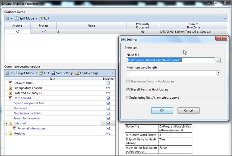
To search the index, you simply go to the Search tab and begin your search. The Search tab, as you recall, can be accessed from the View menu on the application toolbar. The default tab for the Search tab will be, normally, the last tab you used. So, if the Index tab is not the active tab, switch to the Index tab, and your screen should appear as in Figure 7-96.
Figure 7-96: Search tab with Index tab selected
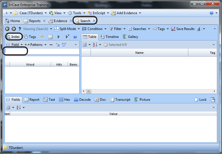
To begin a search, you need only type the keyword into the search string field where, by default, the cursor is located. As type in the keyword, the area below the keyword is dynamically populated with various iterations of the keyword, the number of objects in which it exists, and the total number of hits. For example, as I typed in steganography, EnCase reports the various hits in which steganography is the root of the string, as shown in Figure 7-97.
Figure 7-97: As a keyword is entered, a dynamic list of hits and items is created below.
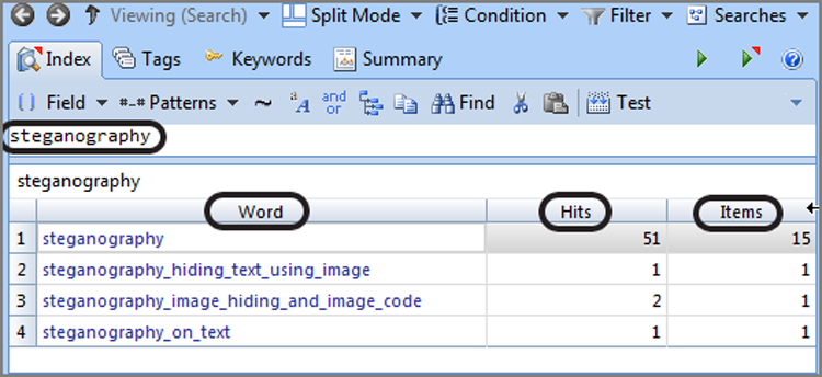
Once you are satisfied with your keyword, you run the query by clicking the play icon on the toolbar, which is circled in Figure 7-98, and the results are displayed in the Table view pane to the right. The Table pane lists the various items in which the keyword appears. You can easily browse the list, selecting various items and viewing the contents below in the various View pane tabs.
Figure 7-98: To run the query, click the Play icon, which is circled.
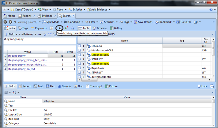
From the View pane, you have many viewing options, which include Text, Hex, Decode, Doc, Transcript, and Picture. Which view will be dictated by user preferences and viewing needs. To navigate between search hits, there are two icons immediately to the right of the Find Next icon. As shown in Figure 7-99, they enable you to sequence between search hits in either direction. To the right of these two buttons are two icons that are labeled Previous Item and Next Item. As the name implies, you can sequence through the items in the Table view pane with these two navigational aids. Finally, don’t forget that you can use the Find and Find Next features to search within the text or beyond, including GREP searches.
As with keyword searches, you can bookmark raw text or notable files from the Search tab panes. Also, if you need to, you can use the Go To File feature. This is a very handy feature for viewing the file in a Tree pane. While in the Search tab Table pane, right-click a file of interest, and choose Go To File, as shown in Figure 7-100. When you do, the chosen file will open in its own Entries tab within the Search tab. To return to the Index tab, use the green left-arrow at the far-left side of the toolbar under the Home icon.
Figure 7-99: Next Hit and Previous Hit buttons enable quick sequencing between search hits.
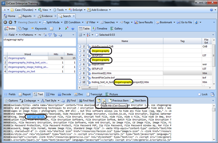
Figure 7-100: Go To File feature
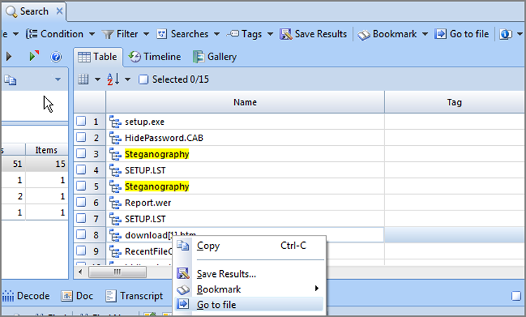
You are not limited to simple keywords with index searches. You can combine keywords with AND or OR logic. You can simply type AND or OR between the keywords, and it will turn blue, indicating it is being recognized as a Boolean logic operator, as shown in Figure 7-101. There is also an AND/OR button on the toolbar that will autofill either of those two words in the event you forget how to spell them. With AND logic, the query will return items that have both keywords, whereas with OR logic, the query will return items with either keyword.
Figure 7-101: Using Boolean AND/OR logic with keywords. In this case, AND logic required both keywords to be present in an item to return a successful query.
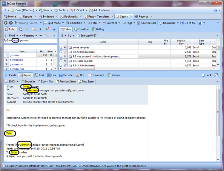
In addition to Boolean search operators, EnCase 7 has many other search operators. Proximity searches are very useful where you are trying to find one keyword near another keyword. The w/# operator is used to find one keyword within a specified number of words from another. For example, steve w/3 bunting will find items in which steve is within three words of bunting, no matter what order.
You can force ordering, however, by using a “one word before the other” operator. For example, steve pre/3 bunting would find items in which steve appeared before bunting and within three words, but it would not find buntingpreceding steve by three words.
Instead of finding words close to one another, we can also go in the other direction, using a “keywords apart from each other” operator. Thus, we specify that keywords can’t be within a specified number of words from each other. For example, steve nw/3 bunting would find only items in which steve and bunting existed more than three words from one another. If ordering were desired, steve npre/3 bunting would force the same conditions, but steve would have to precede bunting and be more than three words apart.
You may have noted that I spelled my name with all lowercase letters in the previous examples because case does not matter with index searches, unless you force the condition. On the toolbar, immediately to the left of the AND/OR logic button, you will find an a/A button. Clicking it will alternately insert a case-sensitive <c> or case-insensitive operator <c-> into the search string, as shown below in Figure 7-102. When the case sensitive operator is used, the search string must match both the string and case, as also shown in Figure 7-102.
Figure 7-102: Case sensitivity operator in use
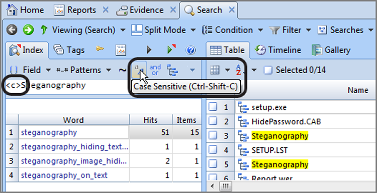
There are many more search operators that apply to index searches, and they change as improvements are made and capabilities enhanced. I suggest visiting the EnCase help feature, as shown in Figure 7-103; on the Contents tab, see Searching Through Evidence > Searching Indexed Data > Search Operators for a listing of the various operators along with helpful examples.
There are times when saving a search is desired, which usually means you want to run the search again in the future and don’t want to take the time to re-create the search terms and logic. Also, you may be operating under strict searching guidelines that were crafted by attorneys arguing for days at their billable rates. In those cases, you want to apply the exact agreed-upon search criteria repeatedly and to have a record of that search in the event the search criteria is later questioned. Regardless of your underlying reasons for doing so, EnCase provides the mechanism. To save your search, go to the Searches menu on the Search tab and choose Save As, as shown in Figure 7-104. The default location will be Documents\EnCase\Search, which is a global location. If you would prefer to store them with the case, simply change the path. You should give the search file a name that describes the search and click Save. Any time in the future that you want to recall this search, simply go to this same menu and choose Open instead.
Figure 7-103: EnCase help feature with listing of available Search Operators with examples
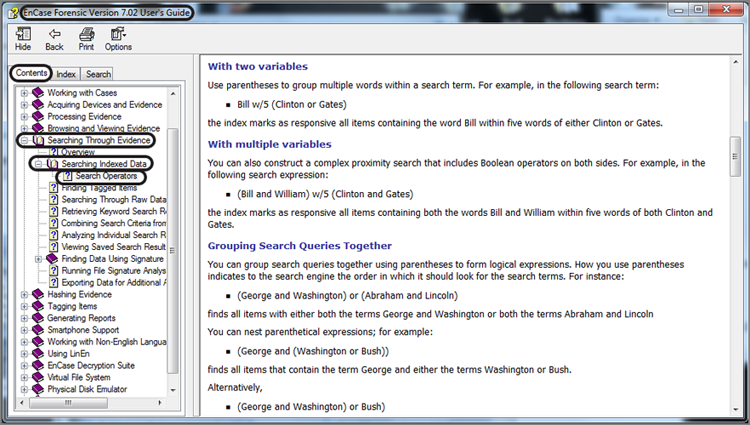
Figure 7-104: Saving a search for later use
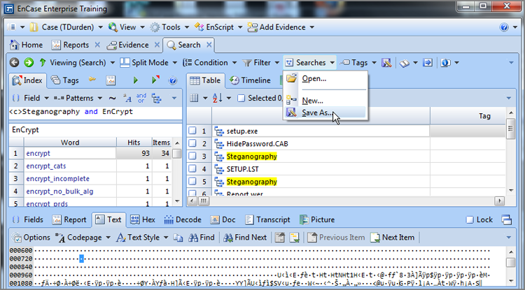
Tags
Thus far, I have not discussed tags. I did not see the point in tags, initially, until I realized that you can search for them, and then their true potential became visible. So, this seems to most appropriate point at which to discuss them. You can apply tags, both default and user-created ones, to items in EnCase and then later search for them from the Search tab. Very quickly, let’s apply a tag and then search for it. Locate any item in the Table view and then locate the Tag column. I would suggest widening the Tags column for reasons that will quickly become obvious. Hold your cursor over the Tag column for any particular item, and you will see the various tags that are available appear as you move your cursor from left to right (or vice versa) within the Tag field, as shown in Figure 7-105. You need only click the desired tag, and the item is so tagged, as shown in Figure 7-106. You can add multiple tags, and you can toggle tags on and off. The Tags menu appears on various toolbars, and you can manage your tags from there, deleting, changing, and creating them as you see fit. I would suggest not having too many because they become rather cumbersome when you do.
Figure 7-105: Passing cursor over Tag field reveals available tags
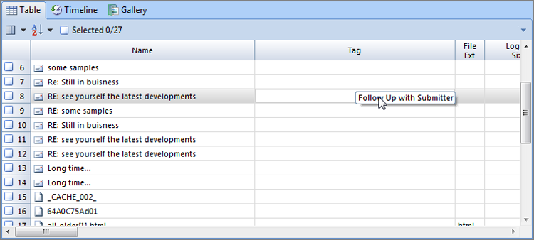
Figure 7-106: An item tagged for “Follow Up”
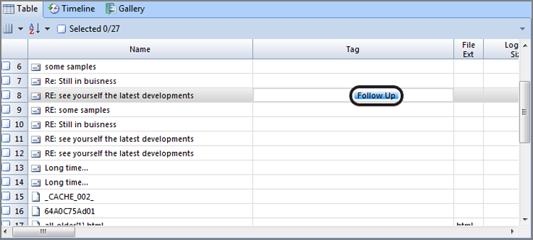
Now you can tag! I mentioned that you can search for them, so let’s switch to the Tags tab in the Search tab. You should immediately see your tag names listed in the left pane. The total number of tagged items for each tag will reflect in the Count column for that particular tag. If the number is zero it is black. If it is other than zero, it will be blue. Since the blue indicates a hyperlink, you need only to click that link to have the items revealed in the Table View pane, as shown in Figure 7-107. Alternatively, you can place a blue check box in the tag’s box and click the Play button. Either method will run the query. You can see in Figure 7-107 that the only item matching my query was the item I just tagged in Figure 7-106.
Figure 7-107: Query returned for tagged items
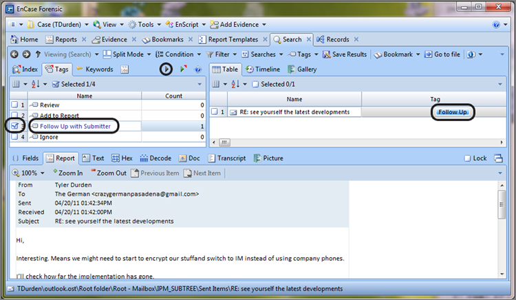
Before we conclude searching, let’s cover two quick items. First is the Results tab. Whenever you run a query, we’ve seen that the results are sent to the Table pane to the right in the Index, Tags, or Keywords tabs, all within the Search tab. Simultaneously, they are also sent to the Results tab, which can be viewed from the View menu. You have a less cluttered interface to work with the results of the query, as shown in Figure 7-108. Some prefer it, and others do not.
Sometimes you may encounter a situation in which you may want to combine an index query with a keyword query or perhaps even a tag query. If you wanted to do so, you could place a blue check mark for the query criteria in each of the tabs (Index, Tags, and/or Keywords) and then activate the query across all tabs with selected items. The button to activate this special query is immediately to the right of the play button and is shown in Figure 7-109. The results will be sent to both the Table pane and the Results tab, as previously mentioned.
Figure 7-108: Queries are also sent to Results tab, which offers a less-cluttered interface for working with search hits.
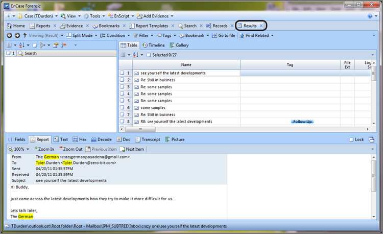
Figure 7-109: Search using combined criteria from all tabs
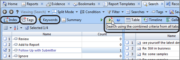
![]()
Do not search for words included in the noise file. If the word the appears in the noise file and you search for the book, EnCase will not return a hit for the book no matter how many times it exists.
Summary
This chapter covered data in its binary and hexadecimal formats. You learned that various storage devices have physical, optical, or electrical states of positive or negative, yes or no, on or off, and so on, that are rendered into 1s and 0s. Binary (base-2) is a system based strictly on 1s and 0s and is the system used by computers to store and transmit data.
A bit is the smallest unit and can have two outcomes, 1 or 0. A byte consists of 8 bits and can have 256 possible outcomes. A byte consists of two 4-bit nibbles. Of those two nibbles, there is a left nibble and a right nibble. Each nibble can have 16 possible outcomes.
Two bytes combined is called a word, which is 16 bits. Four bytes combined is called a Dword, which is 32 bits. Larger still is a Qword, which is four words and 64 bits.
Hexadecimal is a programmer’s shortcut for expressing binary numbers. Each nibble of the byte is evaluated separately. Because each nibble can have 16 possible outcomes, those integer values are represented by a single character ranging from 0 to F (0, 1, 2, 3, 4, 5, 6, 7, 8, 9, A, B, C, D, E, F), which represents the integers 0-16, respectively. Each nibble is represented by a single character, and the two characters are combined to represent the entire byte.
ASCII was originally a 7-bit character set consisting of 128 of the common numbers, characters, and special characters. It is also called low-bit ASCII. To include some foreign languages, graphics, and math symbols, this character set was expanded to an extended 8-bit character chart. It consists of 256 characters and is often called high-bit ASCII.
As computing became global, the world’s varied languages could not be expressed in a 256-character set. Unicode evolved to remedy this situation, allowing 2 bytes per character.
Best practices call for evidence file verification and adjustment of time zone offsets as the first steps after adding evidence to a case. The next step in the process, normally, is to run the EnCase Evidence Processor, which carries out many essential preprocessing tasks, such as recovering folders, analyzing file signatures, analyzing hashes, building a text index, and other tasks.
EnCase 7 has a powerful indexing engine for carrying out index searches, by which you can conduct searches against an index for near-instantaneous search results. Before you can do such a search, you must first create the index. The index is created when you run the EnCase Evidence Processor, which is new to EnCase 7.
EnCase uses keywords as search stings by which to conduct searches. Keywords can be created individually or in groups using keyword lists. Keywords can be imported from EnCase keywords that were exported.
When searching, you create and select keywords by which to search. You also select the data on which the search is to be conducted. You have various options when searching, such as case-sensitive searches, Unicode searches, and others. You can create specialized code pages for foreign-language searches.
Another type of search option is a GREP search. GREP searches allow special characters to be used to construct search terms that can greatly enhance your searching capabilities.
Keyword searches are carried out from the Raw Search menu or can be carried out from the EnCase Evidence Processor. Index searches are carried out from the Index tab of the Search tab.
Once a raw search has been conducted, the results are sent to the Table pane of the Keywords tab and to the Results tab. Search hits can be sorted in the Table view pane.
Files containing search hits can be tagged for further analysis in the Case view. Files containing search hits can be bookmarked from the Search Hits view.
Files or items can be tagged using default tags or user-created tags. Once tagged, items can be searched by those tags on the Search tab.
There are several types of bookmarks. One of the most common and feature-rich bookmarks is the highlighted data bookmark. Using this bookmark, data can be viewed in vast array of formats. The destination folder can be selected, created, or rearranged.
Files can be bookmarked individually as notable file bookmarks or in groups of files that have been selected. Table views can be bookmark using a special bookmark type, named a Table view bookmark. If data is viewed using the Decode tab, the results of the decoding process can be bookmarked using the Data Structure bookmark. Bookmarks are linked to the EnCase report; however, the link may not be automatic, depending on where the bookmark is placed. If a new folder or subfolder is created, the examiner may have to go to the Reports Template and edit the section to link the bookmark folder to a particular section in the report. Metadata for bookmarked files in reports can also be modified in the Reports Template, specifically in a particular section’s formatting options for each bookmark type.
Bookmarks can be moved, deleted, or rearranged. Bookmarks are the foundation from which reports are generated. Creating a well-organized tree of bookmarks with meaningful folder names is essential to creating a good report. When a report is customized, it can be saved as a template, and future cases can benefit from less input during case setup and later with a customized professionally appearing report.
Examiners should take the time necessary to learn to create well-designed and well-organized bookmarks because they translate into well-designed and well-organized reports.
Exam Essentials
Understand binary data concepts. Understand and explain how binary data is stored and translated into human-readable text and numbers. Be able to interpret a binary byte into its hexadecimal format. Understand hexadecimal representation and be able to convert between binary, hexadecimal, and decimal formats. Be able to interpret a binary byte into its integer or ASCII value.
Know and understand the ASCII and Unicode character sets. Explain what the 7-bit low-bit ASCII character set is. Explain what the 8-bit high-bit extended ASCII character set is and how it evolved. Explain how a given hex value could be a character in one context but an integer in another context. Understand and explain the difference between 09h (decimal integer 9) and 39h (printed character 9).
Understand how Unicode evolved and how many bytes are used to represent one character. Know how many characters can be represented by Unicode.
Understand keywords and their implementation into the search process. Explain how to create keywords. Understand and be able to explain how keyword searches can be saved. Be able to export and import keywords. Understand the importance of naming keywords.
Understand GREP search expressions. Know and be able to explain what GREP means. Be able to create GREP expressions to search for specified search strings. Given a GREP expression, be able to determine which strings will match and which strings will not match. Know the purpose and function of the keyword tester.
Know and understand how to conduct searches. Understand and be able to explain how to conduct a raw search in EnCase. Know what search options are available from the Raw Search menu and how they affect the search results.
Understand the Search Tab and the various tabs thereunder. Understand and explain the features and functions available in the Search Tab view. Explain the various tabs in this view and their purpose. Explain how files containing search hits are bookmarked or tagged.
Know and understand how to create bookmarks. Understand and be able to describe what a bookmark is and how to create each bookmark type. Understand how to decode data from a highlighted data bookmark and what the various view types are. Explain how to select destination folders. Explain the importance of organizing folders into a meaningful hierarchical format with folder names that describe their contents. Explain how to move folders and bookmarks. Describe how a report is generated and how bookmarks are linked to reports. Explain the purpose of the report template and some of the functions that can be carried out in that view. Understand the various formats by which reports can be exported or saved. Explain the process of generating a paperless report.
Know and understand how to run the EnCase Evidence Processor. Understand and be able to describe how to launch the EnCase Evidence Processor. Explain the function and importance of processing items with a red flag. Describe the various functions and features of the processing options available in this interface. Explain how to acquire while running the EnCase Evidence Processor.
Know and understand how to conduct an index search. Understand and be able to describe how to create an index and explain the options for creating the index. Know where the index file is stored and how its location is configured. Describe how to query an index from the Index tab. Explain the various search operators and know the syntax for the common types. Explain a noise file. Explain the function and features of the Results tab.
Review Questions
1. Computers use a numbering system with only two digits, 0 and 1. This system is referred to as which of the following?
A. Hexadecimal
B. ASCII
C. Binary
D. FAT
2. A bit can have a binary value of which of the following?
A. 0 or 1
B. 0-9
C. 0-9 and A-F
D. On or Off
3. A byte consists of ___ bits.
A. 2
B. 4
C. 8
D. 16
4. If 1 bit can have two unique possibilities, 2 bits can have four unique possibilities, and 3 bits can have eight unique possibilities. This is known as the power of 2. How many unique possibilities are there in 8 bits (28)?
A. 16
B. 64
C. 128
D. 256
5. When the letter A is represented as 41h, it is displayed in which of the following?
A. Hexadecimal
B. ASCII
C. Binary
D. Decimal
6. What is the decimal integer value for the binary code 0000-1001?
A. 7
B. 9
C. 11
D. 1001
7. Select all of the following that depict a Dword value.
A. 0000 0001
B. 0001
C. FF 00 10 AF
D. 0000 0000 0000 0000 0000 0000 0000 0001
8. How many characters can be addressed by the 7-bit ASCII character table? 16-bit Unicode?
A. 64 and 256
B. 128 and 256
C. 64 and 65,536
D. 128 and 65,536
9. Which of the following are untrue with regard to the EnCase Evidence Processor?
A. A device must be acquired first before processing or be acquired as a requisite first step within the EnCase Evidence Processor.
B. A live device can be subjected to normal processing by the EnCase Evidence Processor and does not have to be acquired first.
C. Items marked with red flags denote items that are not applicable to the file system being processed.
D. Items marked with red flags denote items that must be run during the first or initial run of the EnCase Evidence Processor and can’t be run in any subsequent run thereafter.
E. A raw keyword search can be conducted during processing by the EnCase Evidence Processor.
10. When performing a keyword search in Windows, EnCase searches which of the following?
A. The logical files
B. The physical disk in unallocated clusters and other unused disk areas
C. Both A and B
D. None of the above
11. By default, search terms are case sensitive.
A. True
B. False
12. By selecting the Unicode box for a raw search, EnCase searches for both ASCII and Unicode formats.
A. True
B. False
13. With regard to a search using EnCase in the Windows environment, can EnCase find a word or phrase that is fragmented or spans in noncontiguous clusters?
A. No, because the letters are located in noncontiguous clusters.
B. No, EnCase performs a physical search only.
C. No, unless the File Slack option is deselected in the dialog box before the search.
D. Yes, EnCase performs both physical and logical searches.
14. Which of the following would be a raw search hit for the His keyword?
A. this
B. His
C. history
D. Bill_Chisholm@gmail.com
E. All of the above
15. Which of the following would be a search hit for the following GREP expression?
[^a-z]Liz[^a-z]
A. Elizabeth
B. Lizzy
C. Liz1
D. None of the above
16. Which of the following would be a search hit for the following GREP expression?
[\x00-\x07]\x00\x00\x00…
A. 00 00 00 01 A0 EE F1
B. 06 00 00 00 A0 EE F1
C. 0A 00 00 00 A0 EE F1
D. 08 00 00 00 A0 EE F1
17. Which of the following would be a search hit for the following index search expression?
<c>Saddam npre/3 Hussein
A. Saddam Alfonso Adolph Cano Hitler Hussein
B. saddam alfonso adolph cano hitler hussein
C. Saddam Alfonso Hussein Adolph Cano Hitler
D. saddam alfonso hussein adolph cano hitler
E. Hussein Hitler Cano Adolph Alfonso Saddam
F. None of the above
18. Which of the following will not be a search hit for the following GREP expression?
[^#]123[ \-]45[ \-]6789[^#]
A. A1234567890
B. A123 45-6789
C. A123-45-6789
D. A123 45 6789
19. A sweep or highlight of a specific range of text is referred to as which of the following?
A. Table view bookmark
B. Single item bookmark
C. Highlighted data bookmark
D. Notable file bookmark
E. Notes bookmark
20. Which of the following is not correct regarding EnCase 7 index searches?
A. Before searching, the index must first be created using the Create Index EnScript.
B. Before searching, the index must first be created using the EnCase Evidence Processor.
C. All queries are case insensitive regardless of any switches or settings, because that is the nature of all indexed searches.
D. By default, queries are case insensitive but can be configured to be case sensitive.
E. A query for any word in the noise file will not return any items as all words in the noise file are ignored and excluded from the index.
All materials on the site are licensed Creative Commons Attribution-Sharealike 3.0 Unported CC BY-SA 3.0 & GNU Free Documentation License (GFDL)
If you are the copyright holder of any material contained on our site and intend to remove it, please contact our site administrator for approval.
© 2016-2026 All site design rights belong to S.Y.A.