Network Security Through Data Analysis: Building Situational Awareness (2014)

Part I. Data

Chapter 2. Network Sensors

A network sensor collects data directly from network traffic without the agency of an intermediary application, making them different from the host-based sensors discussed in Chapter 3. Examples include NetFlow sensors on a router and sensors that collect traffic using a sniffing tool such astcpdump.

The challenge of network traffic is the challenge you face with all log data: actual security events are rare, and data costs time and storage space. Where available, log data is preferable because it’s clean (a high-level event is recorded in the log data) and compact. The same event in network traffic would have to be extracted from millions of packets, which can often be redundant, encrypted, or unreadable. At the same time, it is very easy for an attacker to manipulate network traffic and produce legitimate-looking but completely bogus sessions on the wire. An event summed up in a 300-byte log record could easily be megabytes of packet data, wherein only the first 10 packets have any analytic value.

That’s the bad news. The good news is that network traffic’s “protocol agnosticism,” for lack of a better term, means that it is also your best source for identifying blind spots in your auditing. Host-based collection systems require knowing that the host exists in the first place, and there are numerous cases where you’re likely not to know that a particular service is running until you see its traffic on the wire. Network traffic provides a view of the network with minimal assumptions—it tells you about hosts on the network you don’t know existed, backdoors you weren’t aware of, attackers already inside your border, and routes through your network you never considered. At the same time, when you face a zero-day vulnerability or new malware, packet data may be the only data source you have.

The remainder of this chapter is broken down as follows. The next section covers network vantage: how packets move through a network and how to take advantage of that when instrumenting the network. The next section covers tcpdump, the fundamental network traffic capture protocol, and provides recipes for sampling packets, filtering them, and manipulating their length. The section after that covers NetFlow, a powerful traffic summarization approach that provides high-value, compact summary information about network traffic. At the end of the chapter, we look at a sample network and discuss how to take advantage of the different collection strategies.

Network Layering and Its Impact on Instrumentation

Computer networks are designed in layers. A layer is an abstraction of a set of network functionality intended to hide the mechanics and finer implementation details. Ideally, each layer is a discrete entity; the implementation at one layer can be swapped out with another implementation and not impact the higher layers. For example, the Internet Protocol (IP) resides on layer 3 in the OSI model; an IP implementation can run identically on different layer 2 protocols such as Ethernet or FDDI.

There are a number of different layering models. The most common ones in use are the OSI’s seven layer model and TCP/IP’s four layer model. Figure 2-1 shows these two models, representative protocols, and their relationship to sensor domains as defined in Chapter 1. As Figure 2-1shows, the OSI model and TCP/IP model have a rough correspondence. OSI uses the following seven layers:

1. Physical: The physical layer is composed of the mechanical components used to connect the network together—the wires, cables, radio waves, and other mechanisms used to transfer data from one location to the next.

2. Data link: The data link layer is concerned with managing information that is transferred across the physical layer. Data link protocols, such as Ethernet, ensure that asynchronous communications are relayed correctly. In the IP model, the data link and physical layers are grouped together as the link layer.

3. Network: The network layer is concerned with the routing of traffic from one data link to another. In the IP model, the network layer directly corresponds to layer 2, the Internet layer.

4. Transport: The transport layer is concerned with managing information that is transferred across the network layer. It has similar concerns to the data link layer, such as flow control and reliable data transmission, albeit at a different scale. In the IP model, the transport layer is layer 3.

5. Session: The session layer is concerned with the establishment and maintenance of a session, and is focused on issues such as authentication. The most common example of a session layer protocol today is SSL, the encryption and authentication layer used by HTTP, SMTP, and many other services to secure communications.

6. Presentation: The presentation layer encodes information for display at a higher level. A common example of a presentation layer is MIME, the message encoding protocol used in email.

7. Application: The application layer is the service, such as HTTP, DNS, and SSH. OSI layers 5 through 7 correspond roughly to the application layer (layer 4) of the IP model.

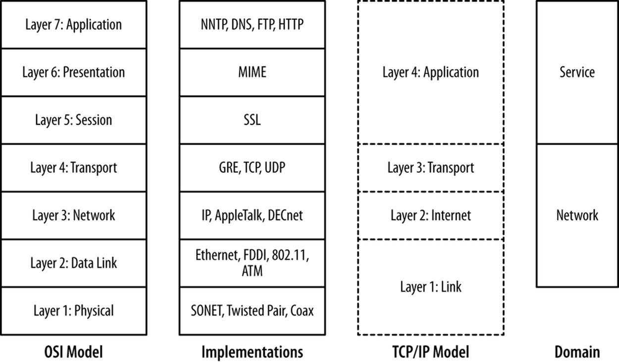
Figure 2-1. Layering models

The layering model is just that: a model rather than a specification, and models are necessarily imperfect. The TCP/IP model, for example, eschews the finer details of the OSI model, and there are a number of cases where protocols in the OSI model might exist in multiple layers. Network interface controllers (NICs) dwell on layers 1 and 2 in the model. The layers do impact each other, in particular through how data is transported (and is observable), and by introducing performance constraints into higher levels.

The most common place where we encounter the impact of layering on network traffic is the maximum transmission unit (MTU). The MTU is an upper limit on the size of a data frame, and impacts the maximum size of a packet that can be sent over that medium. The MTU for Ethernet is 1,500 bytes, and this constraint means that IP packets will almost never exceed that size.

The layering model also provides us with a clear difference between the network and service-based sensor domains. As Figure 2-1 shows, network sensors are focused on layers 2 through 4 in the OSI model, while service sensors are focused on layers 5 and above.

LAYERING AND THE ROLE OF NETWORK SENSORS

It’s logical to ask why network sensors can’t monitor everything; after all, we’re talking about attacks that happen over a network. In addition, network sensors can’t be tampered with or deleted like host logs, and they will see things like scans or failed connection attempts that host logs won’t.

Network sensors provide extensive coverage, but recovering exactly what happened from that coverage becomes more complex as you move higher up the OSI model. At layer 5 and above, issues of protocol and packet interpretation become increasingly prominent. Session encryption becomes an option at layer 5, and encrypted sessions will be unreadable. At layer 6 and layer 7, you need to know the intricacies of the actual protocol that’s being used in order to extract meaningful information.

Protocol reconstruction from packet data is complex and ambiguous; TCP/IP is designed on end-to-end principles, meaning that the server and client are the only parties required to be able to construct a session from packets. Tools such as Wireshark (described in Chapter 9) or NetWitness can reconstruct the contents of a session, but these are approximations of what actually happened.

Network, host, and service sensors are best used to complement each other. Network sensors provide information that the other sensors won’t record, while the host and service sensors record the actual event.

Recall from Chapter 1 that a sensor’s vantage refers to the traffic that a particular sensor observes. In the case of computer networks, the vantage refers to the packets that a sensor observes either by virtue of transmitting the packets itself (via a switch or a router) or by eavesdropping (within a collision domain). Since correctly modeling vantage is necessary to efficiently instrument networks, we need to dive a bit into the mechanics of how networks operate.

Network Layers and Vantage

Network vantage is best described by considering how traffic travels at three different layers of the OSI model. These layers are across a shared bus or collision domain (layer 1), over network switches (layer 2), or using routing hardware (layer 3). Each layer provides different forms of vantage and mechanisms for implementing the same.

The most basic form of networking is across a collision domain. A collision domain is a shared resource used by one or more networking interfaces to transmit data. Examples of collision domains include a network hub or the channel used by a wireless router. A collision domain is called such because the individual elements can potentially send data at the same time, resulting in a collision; layer 2 protocols include mechanisms to compensate for or prevent collisions.

The net result is that layer 2 datagrams are broadcast across a common source, as seen in Figure 2-2. Network interfaces on the same collision domain all see the same datagrams; they elect to only interpret datagrams that are addressed to them. Network capture tools like tcpdump can be placed in promiscuous mode and will then record all the datagrams observed within the collision domain.

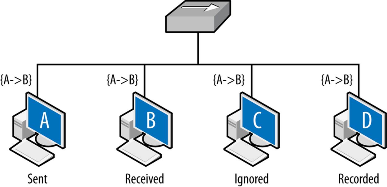
Figure 2-2. Vantage across collision domains

Figure 2-2 shows the vantage across a broadcast domain. As seen in this figure, the initial frame (A to B) is broadcast across the hub, which operates as a shared bus. Every host connected to the hub can receive and react to the frames, but only B should do so. C, a compliant host, ignores and drops the frame. D, a host operating in promiscuous mode, records the frame. The vantage of a hub is consequently all the addresses connected to that hub.

Shared collision domains are inefficient, especially with asynchronous protocols such as Ethernet. Consequently, layer 2 hardware such as Ethernet switches are commonly used to ensure that each host connected to the network has its own dedicated Ethernet port. This is shown in Figure 2-3.

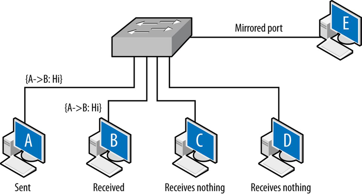
Figure 2-3. Vantage across a switch

A capture tool operating in promiscuous mode will copy every frame that is received at the interface, but the layer 2 switch ensures that the only frames an interface receives are the ones explicitly addressed to it. Consequently, as seen in Figure 2-3, the A to B frame is received by B, while C and D receive nothing.

There is a hardware-based solution to this problem. Most switches implement some form of port mirroring. Port mirroring configurations copy the frames sent between different ports to common mirrored ports in addition to their original destination. Using mirroring, you can configure the switch to send a copy of every frame received by the switch to a common interface. Port mirroring can be an expensive operation, however, and most switches limit the amount of interfaces or VLANs monitored.

Switch vantage is a function of the port and the configuration of the switch. By default, the vantage of any individual port will be exclusively traffic originating from or going to the interface connected to the port. A mirrored port will have the vantage of the ports it is configured to mirror.

Layer 3, when routing becomes a concern, is when vantage becomes messy. Routing is a semiautonomous process that administrators can configure, but is designed to provide some degree of localized automation in order to provide reliability. In addition, routing has performance and reliability features, such as the TTL, which can also impact monitoring.

Layer 3 vantage at its simplest operates like layer 2 vantage. Like switches, routers send traffic across specific ports. Routers can be configured with mirroring-like functionality, although the exact terminology differs based on the router manufacturer. The primary difference is that while layer 2 is concerned with individual Ethernet addresses, at layer 3 the interfaces are generally concerned with blocks of IP addresses because the router interfaces are usually connected via switches or hubs to dozens of hosts.

Layer 3 vantage becomes more complex when dealing with multihomed interfaces, such as the example shown in Figure 2-4. Up until this point, all vantages discussed in this book have been symmetric—if instrumenting a point enables you to see traffic from A to B, it also enables you to see traffic from B to A. A multihomed host like a router has multiple interfaces that traffic can enter or exit.

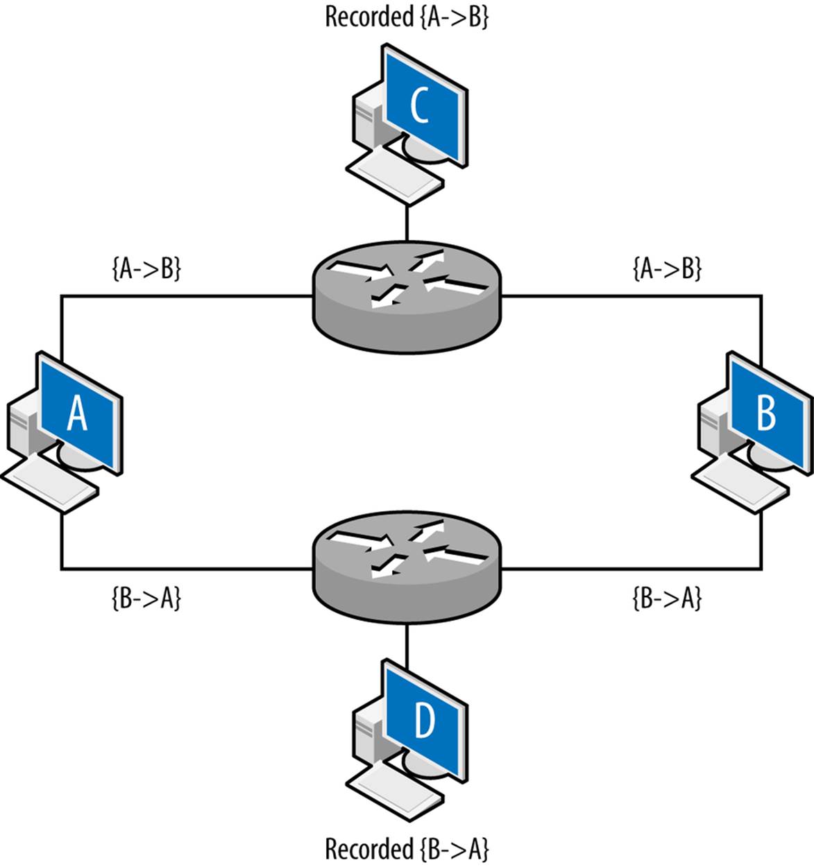
Figure 2-4. Vantage when dealing with multiple interfaces

Figure 2-4 shows an example of multiple interfaces and their potential impact on vantage at layer 3. In this example, A and B are communicating with each other: A sends the packet {A→B} to B, B sends the packet {B→A} to A. C and D are monitoring at the routers: router 1 is configured so that the shortest path from A to B is through it. Router 2 is configured so that shortest path from B to A is through it. The net effect of this configuration is that the vantages at C and D are asymmetric. C will see traffic from A to B, D will see traffic from B to A, but neither of them will see both sides of the interaction. While this example is contrived, this kind of configuration can appear due to business relationships and network instabilities. It’s especially problematic when dealing with networks that have multiple interfaces to the Internet.

IP packets have a built-in expiration function: a field called the time-to-live (TTL) value. The TTL is decremented every time a packet crosses a router (not a layer 2 facility like a switch), until the TTL reaches zero. In most cases, the TTL should not be a problem—most modern stacks set the TTL to at least 64, which is considerably longer than the number of hops required to cross the entire Internet. However, the TTL is manually modifiable and there exist attacks that can use the TTL for evasion purposes. Table 2-1 lists default TTLs by operating system.

Table 2-1. Default TTLs by operating system

Figure 2-5 shows how the TTL operates. Assume that hosts C and D are operating on monitoring ports and the packet is going from A to B. Furthermore, the TTL of the packet is set to 2 initially. The first router receives the packet and passes it to the second router. The second router drops the packet; otherwise, it would decrement the TTL to zero. TTL does not directly impact vantage, but instead introduces an erratic type of blind spot—packets can be seen by one sensor, but not by another several routers later as the TTL decrements.

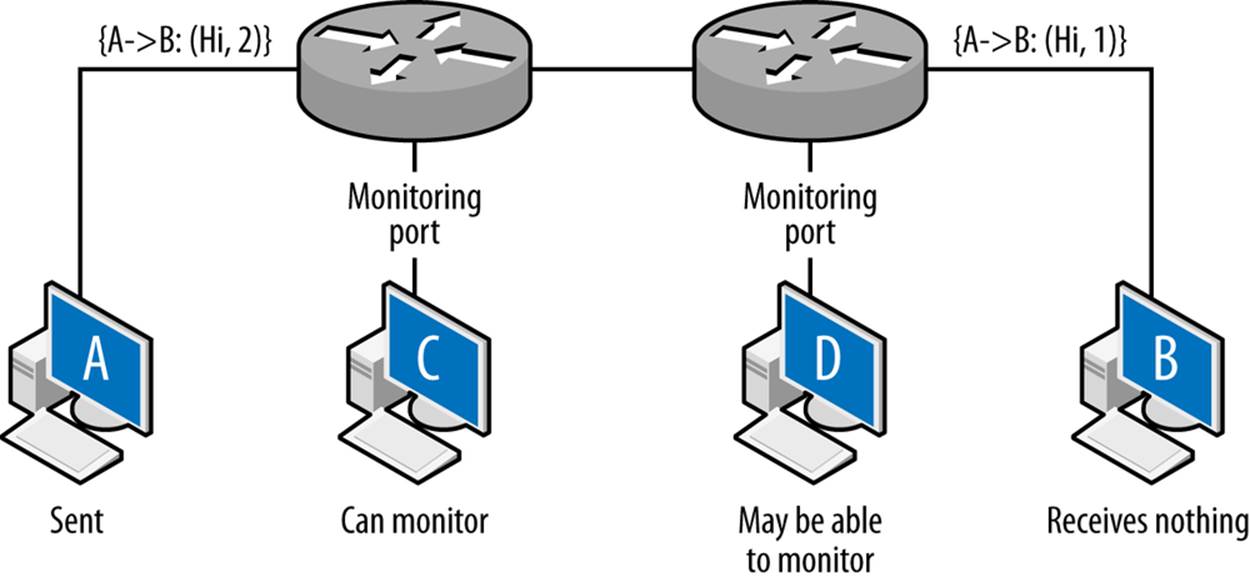
Figure 2-5. Hopping and router vantage

The net result of this is that the packet is observed by C, never received by B, and possibly (depending on the router configuration) observed at D.

PHYSICAL TAPS

Instead of configuring the networking hardware to report data on a dedicated interface, you can monitor the cables themselves. This is done using network taps, which are objects that physically connect to the cables and duplicate traffic for monitoring purposes. Network taps have the advantage of moving the process of collecting and copying data off the network hardware, but only have the vantage of the cables to which they connect.

Network Layers and Addressing

Entities on a network will have multiple addresses that can be used to reach them. For example, the host www.mysite.com may have the IP address 196.168.1.1 and the Ethernet Address 0F:2A:32:AA:2B:14. These addresses are used to resolve the identity of a host at different abstraction layers of the network. In most networks, a host will have a MAC (Ethernet) address and an IPv4 or IPv6 address.

These addresses are dynamically moderated through various protocols, and various types of networking hardware will modify the relationships between addresses. The most common examples of these are DNS modifications, which associate a single name with multiple addresses and vice versa; this is discussed in more depth in Chapter 8. The following addresses are commonly used on networks:

MAC address

A 48-byte identifier used by the majority of layer 2 protocols, including Ethernet, FDDI, Token Ring, Bluetooth, and ATM. MAC addresses are usually recorded as a set of six hexadecimal pairs (e.g., 12:34:56:78:9A:BC). MAC addresses are assigned to the hardware by the original manufacturer, and the first 24 bits of the interface are reserved as a manufacturer ID. As layer 2 addresses, MAC addresses don’t route; when a frame is transferred across a router, the addressing information is replaced with the addressing information of the router’s interface. IPv4 and IPv6 addresses are related to MAC addresses using Address Resolution Protocol (ARP).

IPv4 address

An IPv4 address is a 32-bit integer value assigned to every routable host, with exceptions made for reserved dynamic address spaces (see Chapter 8 for more information on these addresses). IPv4 addresses are most commonly represented in dotted quad format: four integers between 0 and 255 separated by periods (e.g., 128.1.11.3).

IPv6 address

IPv6 is the steadily advancing replacement for IPv4 that fixes a number of design flaws in the original protocol, in particular the allotment of IP addresses. IPv6 uses a 128-bit address to identify a host. By default, these addresses are described as a set of 16-bit hexadecimal values separated by colons (e.g., AAAA:2134:0918:F23A:A13F:2199:FABE:FAAF). Given their length, IPv6 addresses use a number of conventions to shorten the representation: initial zeroes are trimmed, and the longest sequence of 16-bit zero values is eliminated and replaced by double colons (e.g., 0019:0000:0000:0000:0000:0000:0000:0182 becomes 19::182).

All of these relationships are dynamic, and multiple addresses at one layer can be associated with one address at a another layer. As discussed earlier, a single DNS name can be associated with multiple IP addresses through the agency of the DNS service. Similarly, a single MAC address can support multiple IP addresses through the agency of the ARP protocol. This type of dynamism can be used constructively (like for tunneling) and destructively (like for spoofing).

Packet Data

In the context of this book, packet data really means the output of libpcap, either through an IDS or tcpdump. Originally developed by LBNL’s Network Research Group, libpcap is the fundamental network capture tool and serves as the collector for tools such as Snort, bro, and tcpdump.

Packet capture data is a large haystack with only scattered needles of value to you. Capturing this data requires balancing between the huge amount of data that can be captured and the data that it makes sense to actually capture.

Packet and Frame Formats

On almost any modern system, tcpdump will be capturing IP over Ethernet, meaning that the data actually captured by libpcap consists of Ethernet frames containing IP packets. While IP contains over 80 unique protocols, on any operational network, the overwhelming majority of traffic will originate from three protocols: TCP (protocol 6), UDP (protocl 17), and ICMP (protocol 1).

While TCP, UDP, and ICMP make up the overwhelming majority of IP traffic, a number of other protocols may appear in networks, in particular if VPNs are used. IANA has a complete list of IP suite protocols. Some notable ones to expect include IPv6 (protocol number 41), GRE (protocol number 47), and ESP (protocol number 50). GRE and ESP are used in VPN traffic.

Full pcap capture is often impractical. The sheer size and redundancy of the data means that it’s difficult to keep any meaningful fraction of network traffic for a reasonable time. There are three major mechanisms for filtering or limiting packet capture data: the use of rolling buffers to keep a timed subsample, manipulating the snap length to capture only a fixed size packet (such as headers), and filtering traffic using BPF or other filtering rules. Each approach is an analytic trade-off that provides different benefits and disadvantages.

Rolling Buffers

A rolling buffer is a location in memory where data is dumped cyclically: information is dropped linearly, and when the buffer is filled up, data is dumped at the beginning of the buffer, and the process repeats. Example 2-1 gives an example of using a rolling buffer with tcpdump. In this example, the process writes approximately 128 MB to disk, and then rotates to a new file. After 32 files are filled (specified by the -W switch), the process restarts.

Example 2-1. Implementing a rolling buffer in tcpdump

host$ tcpdump -i en1 -s 0 -w result -C 128 -W 32

Rolling buffers implement a time horizon on traffic analysis: data is available only as long as it’s in the buffer. For that reason, working with smaller file sizes is recommended, because when you find something aberrant, it needs to be pulled out of the buffers quickly.

Limiting the Data Captured from Each Packet

An alternative to capturing the complete packet is to capture a limited subset of payload, controlled in tcpdump by the snaplen (-s) argument. Snaplen constrains packets to the frame size specified in the argument. If you specify a frame size of at least 68 bytes, you will record the TCP or UDP headers.^[3^] That said, this solution is a poor alternative to NetFlow, which is discussed later in this chapter.

Filtering Specific Types of Packets

An alternative to filtering at the switch is to filter after collecting the traffic at the spanning port. With tcpdump and other tools, this can be easily done using Berkeley Packet Filtering (BPF). BPF allows an operator to specify arbitrarily complex filters, and consequently your possiblities are fairly extensive. Some useful options are described in this section, along with examples. Figure 2-6 provides a breakdown of the headers for Ethernet frames, IP, UDP, ICMP, and TCP.

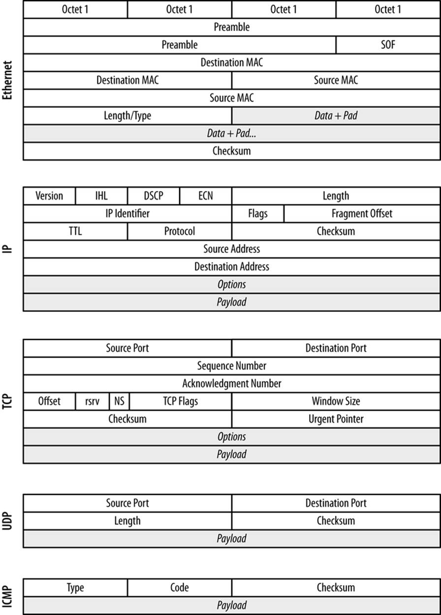
Figure 2-6. Frame and packet formats for Ethernet, IP, TCP, UDP, and ICMP

As we walk through the major fields, I identify BPF macros that describe and can be used to filter on these fields. On most Unix-style systems, the pcap-filter manpage provides a summary of BPF syntax. Available commands are also summarized in the FreeBSD manpage for BPF.

In an Ethernet frame, the most critical fields are the two MAC addresses. These 48-byte fields are used to identify the hardware addresses of the interfaces that sent and will receive the traffic. MAC addresses are restricted to a single collision domain, and will be modified as a packet traverses multiple networks (see Figure 2-5 for an example). MAC addresses are accessed using the ether src and ether dst predicates in BPF.

TCPDUMP AND MAC ADDRESSES

Most implementations of tcpdump require a command-line switch before showing link-level (i.e., Ethernet) information. In Mac OS X, the -e switch will show the MAC addresses.

Within an IP header, the fields you are usually most interested in are the IP addresses, the length, the TTL, and the protocol. The IP identifier, flags, and fragment offset are used for attacks involving packet reassembly—however, they are also largely a historical artifact from before Ethernet was a nearly universal transport protocol. You can get access to the IP addresses using src host and dst host predicates, which also allow filtering on netmasks.

ADDRESS FILTERING IN BPF

Addresses in BPF can be filtered using the various host and net predicates. To understand how these work, consider a simple tcpdump output.

host$ tcpdump -n -r sample.pcap | head -5

reading from file sample.pcap, link-type EN10MB (Ethernet)

20:01:12.094915 IP 192.168.1.3.56305 > 208.78.7.2.389: Flags [S],

seq 265488449, win 65535, options [mss 1460,nop, wscale 3,nop,

nop,TS val 1111716334 ecr 0,sackOK,eol], length 0

20:01:12.094981 IP 192.168.1.3.56302 > 192.168.144.18.389: Flags [S],

seq 1490713463, win 65535, options [mss 1460,nop,wscale 3,nop,

nop,TS val 1111716334 ecr 0,sackOK,eol], length 0

20:01:12.471014 IP 192.168.1.102.7600 > 192.168.1.255.7600: UDP, length 36

20:01:12.861101 IP 192.168.1.6.17784 > 255.255.255.255.17784: UDP, length 27

20:01:12.862487 IP 192.168.1.6.51949 > 255.255.255.255.3483: UDP, length 37

src host or dst host will filter on exact IP addresses; filtering for traffic to or from 192.168.1.3 as shown here:

host$ tcpdump -n -r sample.pcap src host 192.168.1.3 | head -1

reading from file sample.pcap, link-type EN10MB (Ethernet)

20:01:12.094915 IP 192.168.1.3.56305 > 208.78.7.2.389: Flags [S],

seq 265488449, win 65535, options [mss 1460,nop,wscale 3,nop,

nop,TS val 1111716334 ecr 0,sackOK,eol], length 0

host$ tcpdump -n -r sample.pcap dst host 192.168.1.3 | head -1

reading from file sample.pcap, link-type EN10MB (Ethernet)

20:01:13.898712 IP 192.168.1.6.48991 > 192.168.1.3.9000: Flags [S],

seq 2975851986, win 5840, options [mss 1460,sackOK,TS val 911030 ecr 0,

nop,wscale 1], length 0

src net and dst net allow filtering on netblocks. The example below shows how we can progressively filter addresses in the 192.168.1 network using just the address or CIDR notation:

# use src net to filter just by matching octets

host$ tcpdump -n -r sample.pcap src net 192.168.1 | head -3

reading from file sample.pcap, link-type EN10MB (Ethernet)

20:01:12.094915 IP 192.168.1.3.56305 > 208.78.7.2.389: Flags [S],

seq 265488449, win 65535, options [mss 1460,nop,wscale 3,nop,nop,

TS val 1111716334 ecr 0,sackOK,eol], length 0

20:01:12.094981 IP 192.168.1.3.56302 > 192.168.144.18.389: Flags [S],

seq 1490713463, win 65535, options [mss 1460,nop,wscale 3,nop,

nop,TS val 1111716334 ecr 0,sackOK,eol], length 0

# Match an address

host$ tcpdump -n -r sample.pcap src net 192.168.1.5 | head -1

reading from file sample.pcap, link-type EN10MB (Ethernet)

20:01:13.244094 IP 192.168.1.5.50919 > 208.111.133.84.27017: UDP, length 84

# Match using a CIDR block

host$ tcpdump -n -r sample.pcap src net 192.168.1.64/26 | head -1

reading from file sample.pcap, link-type EN10MB (Ethernet)

20:01:12.471014 IP 192.168.1.102.7600 > 192.168.1.255.7600: UDP, length 36

To filter on protocols, use the ip proto predicate. BPF also provides a variety of protocol-specific predicates, such as tcp, udp, and icmp. Packet length can be filtered using the less and greater predicates, while filtering on the TTL requires more advanced bit manipulation, which is discussed later.

The following snippet filters out all traffic except that coming within this block (hosts with the netmask /24).

host$ tcpdump -i en1 -s 0 -w result src net 192.168.2.0/24

Example 2-2 demonstrates filtering with tcpdump

Example 2-2. Examples of filtering using tcpdump

host$ # Filtering out everything but internal traffic

host$ tcpdump -i en1 -s 0 -w result src net 192.168.2.0/24 && dst net \

192.168.0.0/16

host$ # Filtering out everything but web traffic, identified by port

host$ tcpdump -i en1 -s 0 -w result ((src port 80 || src port 443) && \

(src net 192.168.2.0))

In TCP, the port number and flags are the most critical. TCP flags are used to maintain the TCP state machine, while the port numbers are used to distinguish sessions and for service identification. Port numbers can be filtered using the src port and dst port switches, as well as the src portrange and dst portrange switches, which filter across a range of port values. BPF supports a variety of predicates for TCP flags, including tcp-fin, tcp-syn, tcp-rst, tcp-push, tcp-ack, and tcp-urg.

ADDRESS CLASSES AND CIDR BLOCKS

An IPv4 address is a 32-bit integer. For convenience, these integers are usually referred to using dotted quad notation like o1.o2.o3.o4, so the IP address represented by 0x000010FF is written as 0.0.16.255. Level 3 routing is almost never done to individual addresses, but instead to groups of addresses—historically, classes, now netblocks.

It used to be that a class A address (0.0.0.0–127.255.255.255) had the high order bit set to zero, the next 7 assigned to an entity, and the remaining 24 bits under the owner’s control. This gave the owner 2²⁴ addresses to work with. A class B address (128.0.0.0–191.255.255.255) assigned 16 bits to the owner, and class C (192.0.0.0–223.255.255.255) assigned 8 bits. This approach led rapidly to address exhaustion, and in 1993, Classless Inter-Domain Routing (CIDR) was developed to replace the naive class system. Under the CIDR scheme, users are assigned a netblock via an address and a netmask. The netmask indicates which bits in the address the user can manipulate, and by convention, those bits are set to zero. For example, a user who owns the addresses 192.28.3.0–192.28.3.255 will be given the block 192.28.3.0/24.

As with TCP, the UDP port numbers are most important, and are accessible using the same port and portrange switches as TCP.

Because ICMP is the Internet’s error-message passing protocol, ICMP messages tend to contain extremely rich data. The ICMP type and code are the most critical because they define the syntax for whatever payload (if any) follows. BPF provides a variety of type and code specific filters, including icmp-echoreply, icmp-unreach, icmp-tstamp, and icmp-redirect.

What If It’s Not Ethernet?

For the sake of brevity, this book focuses exclusively on IP over Ethernet, but you may well encounter a number of other transport and data protocols. The majority of these protocols are highly specialized and may require additional capture software besides the tools built on libpcap.

ATM

Asynchronous Transfer Mode, the great IP slayer of the ’90s, ATM is now largely used for ISDN and PSTN transport, and some legacy installations.

Fibre Channel

Primarily used for high-speed storage, Fibre Channel is the backbone for a variety of SAN implementations.

CAN

Stands for controller area network. Primarily associated with embedded systems such as vehicular networks, CAN is a bus protocol used to send messages in small isolated networks.

Any form of filtering imposes performance costs. Implementing a spanning port on a switch or a router sacrifices performance that the switch or router could be using for traffic. The more complicated a filter is, the more overhead is added by the filtering software. At nontrivial bandwidths, this will be a problem.

NetFlow

NetFlow is a traffic summarization standard developed by Cisco Systems and originally used for network services billing. While not intended for security, NetFlow is fantastically useful for that purpose because it provides a compact summary of network traffic sessions that can be rapidly accessed and contains the highest-value information that you can keep in a relatively compact format. NetFlow has been increasingly used for security analysis since the publication of the original flow-tools package in 1999, and a variety of tools have been developed that provide NetFlow with additional fields, such as selected snippets of payload.

The heart of NetFlow is the concept of a flow, which is an approximation of a TCP session. Recall that TCP sessions are assembled at the endpoint by comparing sequence numbers. Juggling all the sequence numbers involved in multiple TCP sessions is not feasible at a router, but it is possible to make a reasonable approximation using timeouts. A flow is a collection of identically addressed packets that are closely grouped in time.

NetFlow v5 Formats and Fields

NetFlow v5 is the earliest common NetFlow standard, and it’s worth covering the values in NFv5’s fields before discussing alternatives. NetFlow’s fields (listed in Table 2-2) fall into three broad categories: fields copied straight from IP packets, fields summarizing the results of IP packets, and fields related to routing.

Table 2-2. NetFlow v5 fields

The srcaddr, dstaddr, srcport, dstport, prot, and tos fields of a NetFlow record are copied directly from the corresponding fields in IP packets. Flows are generated for every protocol in the IP suite, however, and that means that the srcport and dstport fields, which strictly speaking are TCP/UDP phenomena, don’t necessarily always mean something. In the case of ICMP, NetFlow records the type and code in the dstport field. In the case of other protocols, ignore the value.

The packets, dOctets, first, last, and tcp_flags fields all summarize traffic from one or more packets. packets and dOctets are simple totals, with the caveat that the dOctets value is the layer 3 total of octets, meaning that IP and protocol headers are added in (e.g., a one-packet TCP flow with no payload will be recorded as 40 bytes, and a one-packet UDP flow with no payload as 28 bytes). The first and last values are, respectively, the first and last times observed for a packet in the flow.

tcp_flags is a special case. In NetFlow v5, the tcp_flags field consists of an OR of all the flags that appear in the flow. In well-formed flows, this means that the SYN, FIN, and ACK flags will always be high.

The final set of fields—nexthop, input, output, src_as, dst_as, src_mask, and dst_mask—are all routing-related. These values can be collected only at a router.

“Flow and Stuff:” NetFlow v9 and IPFIX

Cisco developed several versions of NetFlow over its lifetime, with NetFlow v5 ending up as the workhorse implementation of the standard. But v5 is a limited and obsolete standard, focused on IPv4 and designed before flows were commonly used. Cisco’s solution to this was NetFlow v9, a template-based flow reporting standard that enabled router administrators to specify what fields were included in the flow.

Template-based NetFlow has since been standardized by the IETF as IPFIX.^[4^] IPFIX provides several hundred potential fields for flows, which are described in RFC 5102.

The priority of the standard is on network monitoring and traffic analysis rather than information security. To address optional fields, IPFIX has the concept of a “vendor space.” In the course of developing the SiLK toolkit, the CERT Network Situational Awareness Group at Carnegie Mellon University developed a set of security-sensitive fields that are in their IPFIX vendor space and provide a set of useful fields for security analysis.

NetFlow Generation and Collection

NetFlow records are generated directly by networking hardware appliances (e.g., a router or a switch), or by using software to convert packets into flows. Each approach has different trade-offs.

Appliance-based generation means using whatever NetFlow facility is offered by the hardware manufacturer. Different manufacturers use similar sounding but different names than Cisco, such as Jflow by Juniper Networks and NetStream by Huawei. Because NetFlow is offered by so many different manufacturers with a variety of different rules, it’s impossible to provide a technical discussion about the necessary configurations in the space provided by this book. However, the following rules of thumb are worth noting:

§ NetFlow generation can cause performance problems on routers, especially older models. Different companies address this problem in different ways, ranging from reducing the priority of the process (and dropping records), to offloading the NetFlow generation task to optional (and expensive) hardware.

§ Most NetFlow configurations default to some form of sampling in order to reduce the performance load. For security analysis, NetFlow should be configured to provide unsampled records.

§ Many NetFlow configurations offer a number of aggregation and reporting formats. You should collect raw NetFlow, not aggregations.

The alternative to router-based collection is to use an application that generates NetFlow from pcap data, such as the CERT’s Yet Another Flowmeter (YAF) tool, softflowd, or the extensive flow monitoring tools provided by QoSient’s Argus tool. These applications take pcap as files or directly off a network interface and aggregate the packets as flows. These sensors lack a router’s vantage, but at the same time are able to devote more processing resources to analyzing the packets and can produce richer NetFlow output, incorporating features such as deep packet inspection.

Further Reading

1. Richard Bejtlich, The Tao of Network Security Monitoring: Beyond Intrusion Detection (Addison–Wesley, 2004).

2. Kevin Fall and Richard Stevens, TCP/IP Illustrated, Volume 1: The Protocols (2nd Edition) (Addison–Wesley, 2011).

3. Michael Lucas, Network Flow Analysis (No Starch Press, 2010).

4. Radia Perlman, Interconnections: Bridges, Routers, Switches, and Internetworking Protocols (2nd Edition) (Addison–Wesley, 1999).

5. Chris Sanders, Practical Packet Analysis: Using Wireshark to Solve Real-World Problems (No Starch Press, 2011).