Network Security Through Data Analysis: Building Situational Awareness (2014)

Part II. Tools

Chapter 6. An Introduction to R for Security Analysts

R is an open source statistical analysis package developed initially by Ross Ihaka and Robert Gentleman of the University of Auckland. R was designed primarily by statisticians and data analysts, and is related to commercial statistical packages such as S and SPSS. R is a toolkit for exploratory data analysis; it provides statistical modeling and data manipulation capabilities, visualization, and a full-featured programming language.

R fulfills a particular utility knife-like role for analysis. Analytic work requires some tool for creating and manipulating small ad hoc databases that summarize raw data. For example, hour summaries of traffic volume from a particular host broken down by services. These tables are more complex than the raw data but are not intended for final publication—they still require more analysis. Historically, Microsoft Excel has been the workhorse application for this type of analysis. It provides numeric analysis, graphing, and a simple columnar view of data that can be filtered, sorted, and ordered. I’ve seen analysts trade Excel files around like they were scraps of paper.

I switched from Excel to R because I found it to be a superior product for large-scale numerical analysis. The graphical nature of Excel makes it clunky when you deal with significantly sized datasets. I find R’s table manipulation capabilities to be superior, it provides provenance in the form of saveable and sharable workspaces, the visualization capabilities are powerful, and the presence of a full-featured scripting language enables rapid automation. Much of what is discussed in this chapter can be done in Excel, but if you can invest the time to learn R, I believe you’ll find it well spent.

The first half of this chapter focus on accessing and manipulating data using R’s programming environment. The second half focuses on the process of statistical testing using R.

Installation and Setup

R is a well-maintained open source project. The Comprehensive R Archive Network (CRAN) maintains current binaries for Windows, Mac OS X, and Linux systems, an R package repository, and extensive documentation.

The easiest way to install R is to grab the appropriate binary (at the top of the home page). R is also available for every major package manager. For the rest of this chapter, I am going to assume you’re using R within its own graphical interface.

There are a number of other tools available for working with R, depending on the tools and environments you’re comfortable with. RStudio is an integrated development environment providing data, project, and task management tools in a more traditional IDE framework. For Emacs users, Emacs Speaks Statistics or ESS-mode provides an interactive environment.

Basics of the Language

This section is a crash course in R’s language. R is a rich language with a surface I’m barely scratching. However, at the end of this section, you’ll be able to write a simple R program, run it at the command line, and save it as a library.

The R Prompt

Starting R will present you with a window and command prompt. An example R console is shown in Figure 6-1. As this figure shows, the console is dominated by a large text window and a series of buttons at the top that provide supplemental functions. Note the two text fields under the button row. The first shows the current working directory and the second is the help function. R is very well documented, so get used to using that box.

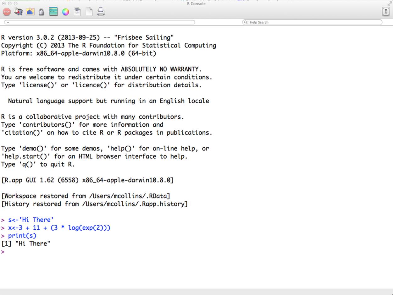
Figure 6-1. The R console

In Figure 6-1, I’ve typed a couple of simple commands, recreated here:

> s<-'Hi There'

> x<- 3 + 11 + (3 * log(exp(2)))

> print(s)

[1] "Hi There"

> print(x)

[1] 20

The command line prompt for R is >; after that, you can enter commands by hand. If a command is partly completed (for example, by opening but not closing parentheses), the next prompt will be a sign, and continue until closure.

> s<- 3 * (

+ 5 + 11

+ + 2

+ )

> s

[1] 54

Note that when R returns a value (for example, the output of s in the previous example), it prints a [1] in square brackets. The value in brackets is an array index; if an array spreads over several lines, the relevant index will be printed at the beginning of each line.

> s<-seq(1,20)

> s

[1] 1 2 3 4 5 6 7 8 9 10 11 12

[13] 13 14 15 16 17 18 19 20

Help can be accessed by using help(term) or ?term. Search through help via help.search() or ??.

To quit R, use the switch icon or the appropriate quit command (Command-Q or Ctrl-Q) for the operating system. If you’re using pure command-line R (i.e., without the graphical interface), you can end the session using Ctrl-D or typing q() at the prompt.

When R terminates, it asks whether you want to save the workspace. Workspace files can be reloaded after a session to continue whatever work that was being done at the time of termination.

R Variables

R supports a number of different data types, including scalar integers, character data (strings), Booleans and floating-point values, vectors, matrices, and lists. The scalar types, as shown in the following example, can be assigned using the ← (“gets”), =, and → operators. R overloads some complicated scoping into its assignment operators, and for our purposes (and almost all R programming), R style guides recommend using the ← operator instead of the = sign.

> # Assign some value directly

> a<-1

> b<-1.0

> c<-'A String'

> d<-T

> # We'll assign e to d

> e<-d

> e

[1] TRUE

> d

[1] TRUE

> # Now we we reassign d, and we see d changes but e remains the same.

> d<-2

> d

[1] 2

> e

[1] TRUE

An R vector is an ordered set of one or more values of the same type: character, logical, or string. Vectors can be created using the c function or any of a number of other functions. Vectors are the most commonly used element in R: the scalar values we used earlier were technically vectors of length 1.^[6^]

> # An example of an integer vector

> int.vec<-c(1,2,3,4,5)

> int.vec

[1] 1 2 3 4 5

> # Floating point numbers will be cast to integer, or integers to floats

> # as needed

> float.vec<-c(1,2.0,3)

> float.vec

[1] 1 2 3

> float.vec<-c(1,2.45,3)

> float.vec

[1] 1.00 2.45 3.00

> # Vectors can also be logical

> logical.vec<-c(T,F,F,T)

> logical.vec

[1] TRUE FALSE FALSE TRUE

> # They will be cast to integers if put into a numeric vector

> mixed.vec<-c(1,2,FALSE,TRUE)

> mixed.vec

[1] 1 2 0 1

> # Character vectors consist of one or more strings; note that a

> #string is a single element

> char.vec <- c("One","Two","Three")

> char.vec

[1] "One" "Two" "Three"

> # Length gives vector lengths

> length(int.vec)

[1] 5

> # Note that the character vector's length is the length of the total

> # number of strings, not the individual characters

> length(char.vec)

[1] 3

Note the length of the character vector: in R, strings are treated as a single element regardless of the number of characters. There are functions for accessing strings—nchar to get the length, and substr and strsplit to extract elements from a string—but individual character strings are not as directly accessible as they are in Python.

R provides a number of functions for vector arithmetic. A vector can be added to or multiplied by another vector; if they’re equally sized, the result will be calculated on an element-by-element basis. If one vector is smaller, it will be repeated to make a vector of equal size. (A vector whose length is not a factor of the other vector will raise an error.) This applies to single-element vectors as well: add a single element to a longer vector and each element in the vector will be added to; multiply and each element will be multiplied.

Vectors are indexable. Individual elements can be accessed using square brackets, so v[k] is the kth element of v. Vectors also support ranged slicing, such as v[a:b]. A negative index will eliminate the indexed element from the vector, like in the following code block:

> # We start by creating a vector out of two others

> v1 <- c(1,2,3,4,5)

> v2 <- c(6,7,8,9,10)

> v3 <- c(v1,v2)

> v3

[1] 1 2 3 4 5 6 7 8 9 10

> # Note that there's no nesting

> # Basic arithmetic - multiplication and addition

> 2 * v1

[1] 2 4 6 8 10

> 2 * v3

[1] 2 4 6 8 10 12 14 16 18 20

> 1 + v1

[1] 2 3 4 5 6

> v1 * v2

# Multiplication

[1] 6 14 24 36 50

# Slicing a range

> v3[1:3]

[1] 1 2 3

# This is identical to v3[1]

> v3[1:1]

[1] 1

> v3[2:4]

[1] 2 3 4

# Reverse the range to reverse the vector

> v3[3:1]

[1] 3 2 1

# Use negative numbers to cut out elements

> v3[-3]

[1] 1 2 4 5 6 7 8 9 10

> v3[-1:-3]

[1] 4 5 6 7 8 9 10

> # You can use logical vectors as selectors; selection returns anything where

> # the index is true

> v3[c(T,F)]

[1] 1 3 5 7 9

R can construct matrices out of vectors using the matrix function. As with vectors, matrices can be added and multiplied (with themselves, vectors, and other matrices), and selected and sliced using a number of different approaches, like those shown here:

> # Matrices are constructed using the matrix commmand, as shown in the

> # basic form below. Note that columns are filled up first.

> s<-matrix(v3,nrow=2,ncol=5)

> s

[,1] [,2] [,3] [,4] [,5]

[1,] 1 3 5 7 9

[2,] 2 4 6 8 10

> # Adding a single element

> s + 3

[,1] [,2] [,3] [,4] [,5]

[1,] 4 6 8 10 12

[2,] 5 7 9 11 13

> # Multiplication

> s * 2

[,1] [,2] [,3] [,4] [,5]

[1,] 2 6 10 14 18

[2,] 4 8 12 16 20

> # Multiplication by a matrix

> s * s

[,1] [,2] [,3] [,4] [,5]

[1,] 1 9 25 49 81

[2,] 4 16 36 64 100

> # Adding a vector, note that addition goes

> # through the columns first

> s + v3

[,1] [,2] [,3] [,4] [,5]

[1,] 2 6 10 14 18

[2,] 4 8 12 16 20

> # Adding a smaller vector, note that

> # it loops over the matrix, column-first

> s + v1

[,1] [,2] [,3] [,4] [,5]

[1,] 2 6 10 9 13

[2,] 4 8 7 11 15

> # Slicing; the use of the comma will strike most people as weird.

> # Before the commma are the rows, after the comma are the columns.

> # The result is returned as a vector, which is why the "column" is now

> # horizontal

> s[,1]

[1] 1 2

> s[1,]

[1] 1 3 5 7 9

> # Accesssing a single element

> s[1,1]

[1] 1

> # Now I'm accessing the 1st and 2nd column elements from the

> # first row; again, get a vector back

> s[1,1:2]

[1] 1 3

> # First and second row elements from the first column

> s[1:2,1]

[1] 1 2

> # Now I get a matrix back because I pull two vectors

> s[1:2,1:2]

[,1] [,2]

[1,] 1 3

[2,] 2 4

> # Selection using booleans, the first value is the row I pull from

> s[c(T,F)]

[1] 1 3 5 7 9

> s[c(F,T)]

[1] 2 4 6 8 10

> # If I specify another vector, it'll pull out columns

> s[c(F,T),c(T,F,T,T,F)]

[1] 2 6 8

An R list is effectively a vector of vector elements, each of which can be composed of its own lists. Lists, like matrices, are constructed with their own special command. Lists can be sliced like a vector, although individual elements are accessed using double brackets. Of more interest, lists can be named; individual vectors can be assigned a name and then accessed using the $ operator.

# Review elements of earlier vectors

> v3

[1] 1 2 3 4 5 6 7 8 9 10

> v4

[1] "Hi" "There" "Kids"

> # Create a list; note that we can add an arbitrary number of elements.

> # Each element added is a new index.

> list.a <- list(v3,v4,c('What','The'),11)

> # Dump the list; note the list indices in double brackets.

> list.a

[[1]]

[1] 1 2 3 4 5 6 7 8 9 10

[[2]]

[1] "Hi" "There" "Kids"

[[3]]

[1] "What" "The"

[[4]]

[1] 11

> # Lists do not support vector arithmetic.

> list.a + 1

Error in list.a + 1 : non-numeric argument to binary operator

> # Individual elements can be examined via indexing. Single brackets

> # return a list.

> list.a[1]

[[1]]

[1] 1 2 3 4 5 6 7 8 9 10

> # Double brackets return the element itself; note that the list index

> # (the [[1]]) isn't present here

> list_a[[1]]

[1] 1 2 3 4 5 6 7 8 9 10

> # The single brackets returned a list, and the double brackets then returned

> # the first element in that single-element list.

> list_a[1][[1]]

[1] 1 2 3 4 5 6 7 8 9 10

> # Access using double brackets, then a single bracket in the vector.

> list_a[[1]][1]

[1] 1

> list_a[[2]][2]

[1] "There"

> # We can modify the results.

> list_a[[2]][2] <- 'Wow'

> # Now we'll create a named list.

> list_b <- list(values=v1,rant=v2,miscellany=c(1,2,3,4,5,9,10))

> # The parameter names become the list element names, and the arguments

> # are the actual elements of the list.

> list_b

$values

[1] 1 2 3 4 5

$rant

[1] 6 7 8 9 10

$miscellany

[1] 1 2 3 4 5 9 10

> # Named elements are accessed using the dollar sign.

> list_b$miscellany

[1] 1 2 3 4 5 9 10

> # After accessing, you can use standard slicing.

> list_b$miscellany[2]

[1] 2

> # Note that the index and the name point to the same value.

> list_b[[3]]

[1] 1 2 3 4 5 9 10

Understanding list syntax is important for data frames, which we discuss in more depth later.

Writing Functions

R functions are created by binding the results of the function command to a symbol, like so:

> add_elements <- function(a,b) a + b

> add_elements(2,3)

[1] 5

> simple_math <- function(x,y,z) {

+ t <- c(x,y)

+ z * t

+ }

Note the curly braces. In R, curly braces are used to hold multiple expressions, and return the final statement of those multiple expressions. Curly braces can be used without a function or anything else, as shown here:

> { 8 + 7

+ 9 + 2

+ c('hi','there')

+ }

[1] "hi" "there"

So, in simple_math, the results in the braces are evaluated sequentially and the final result returned. The final result need not have any relationship to the previous statements within the block. R does have a return statement to control the termination and return of a function, but the convention is not to use it if the results are obvious.

As the examples show, function arguments are defined in the function statement. Arguments can be given a default value by using the = sign; any argument to which you assign a default value becomes optional. Argument assignment can be done through order or by explicitly using the argument name, as shown here:

# Create a function with an optional argument

> test<-function(x,y=10) { x + y }

# If the argument is not passed, R will use the default

> test(1)

[1] 11

> # Call both arguments and values are set positionally

> test(1,5)

[1] 6

> # The value can also be assigned using the argument name

> test(1,y=9)

[1] 10

> # For all variables

> test(x=3,y=3)

[1] 6

> # Names supercede position

> test(y=8,x=4)

[1] 12

> # A value without a default still must be assigned.

> test()

Error in x + y : 'x' is missing

R’s functional features allow you to treat functions as objects that can be manipulated, evaluated, and applied as needed. Functions can be passed to other functions as parameters, and by using the apply and Reduce functions, can be used to support more complex evaluation.

> # Create a function to be called by another function

> inc.func<-function(x) { x + 1 }

> dual.func<-function(y) { y(2) }

> dual.func(inc.func)

[1] 3

> # R has a number of different apply functions based on input type

> # (matrix, list, vector) and output type.

> test.vec<-1:20

> test.vec

[1] 1 2 3 4 5 6 7 8 9 10 11 12 13 14 15 16 17 18 19 20

> # Run sapply on an anonymous function; note that the function isn't bound

> # to an object; it exists for the duration of the run. I could just as

> # easily call sapply(c,inc.func) to use the function inc.func defined above.

> sapply(test.vec,function(x) x+2)

[1] 3 4 5 6 7 8 9 10 11 12 13 14 15 16 17 18 19 20 21 22

> # Where sapply is the classic map function, Reduce is the classic fold/reduce

> # function, reducing a vector a single value. In this case, the function

> # passed adds a and b together, adding the integers 1 to 20 together yields 210

> # Note Reduce's capitalization

> Reduce(function(a,b) a+b,1:20)

[1] 210

A point about loops in R: R’s loops (particularly the for loop) are notoriously slow. Many tasks that would be done with a for loop in Python or C are done in R using a number of functional constructs. sapply and Reduce are the frontend for this.

Conditionals and Iteration

The basic conditional statement in R is if…then…else, using else if to indicate multiple statements. The if statement is itself a function, and returns a value that can be evaluated.

> # A simple if/then which prints out a string

> if (a == b) print("Equivalent") else print("Not Equivalent")

[1] "Not Equivalent"

> # We could just return values directly

> if (a==b) "Equivalent" else "Not Equivalent"

[1] "Not Equivalent"

# If/then is a function, so we can plug it into another function or an if/then

> if((if (a!=b) "Equivalent" else "Not Equivalent") == \

"Not Equivalent") print("Really not equivalent")

> a<-45

> # Chain together multiple if/then statements using else if

> if (a == 5) "Equal to five" else if (a == 20) "Equal to twenty" \

else if (a == 45) "Equal to forty five" else "Odd beastie"

[1] "Equal to forty five"

> a<-5

> if (a == 5) "Equal to five" else if (a == 20) "Equal to twenty" \

else if (a == 45) "Equal to forty five" else "Odd beastie"

[1] "Equal to five"

> a<-97

> if (a == 5) "Equal to five" else if (a == 20) "Equal to twenty" \

else if (a == 45) "Equal to forty five" else "Odd beastie"

[1] "Odd beastie"

R provides a switch statement as a compact alternative to multiple if/then clauses. The switch statement uses positional arguments for integer comparisons, and optional parameter assignments for text comparison.

> # When switch takes a number as its first parameter, it returns the

> # argument with an index that corresponds to that number, so the following

> returns the second argument, "Is"

> switch(2,"This","Is","A","Test")

[1] "Is"

> proto<-'tcp'

> # If parameters are named, those text strings are used for matching

> switch(proto,tcp=6,udp=17,icmp=1)

[1] 6

> # The last parameter is the default argument

> proto<-'unknown'

> switch(proto, tcp=6,udp=17,icmp=1, -1)

[1] -1

> # To use a switch repeatedly, bind it to a function

> proto<-function(x) { switch(x, tcp=6,udp=17,icmp=1)}

> proto('tcp')

[1] 6

> proto('udp')

[1] 17

> proto('icmp')

[1] 1

R has three looping constructs: repeat, which provides infinite loops by default; while, which does a conditional evaluation in each loop; and for, which iterates over a vector. Internal loop operations are controlled by break (which terminates the loop), and next (which skips through an iteration), as seen here:

> # A repeat loop; note that repeat loops run infinitely unless there's a break

> # statement in the loop. If you don't specify a condition, it'll run forever.

> i<-0

> repeat {

+ i <- i + 1

+ print(i)

+ if (i > 4) break;

+ }

[1] 1

[1] 2

[1] 3

[1] 4

[1] 5

> # The while loop with identical functionality; this one doesn't require the

> # break statement

> i <- 1

> while( i < 6) {

+ print(i)

+ i <- i + 1

+ }

[1] 1

[1] 2

[1] 3

[1] 4

[1] 5

> # The for loop is most compact

> s<-1:5

> for(i in s) print(i)

[1] 1

[1] 2

[1] 3

[1] 4

[1] 5

Although R provides these looping constructs, it’s generally better to avoid loops in favor of functional operations such as sapply. R is not a general purpose programming language; it was explicitly designed to provide statistical analysts with a rich toolkit of operations. R contains an enormous number of optimized functions and other tools available for manipulating data. We cover some later in this chapter, but a good R reference source is invaluable.

Using the R Workspace

R provides users with a persistent workspace, meaning that when a user exits an R session, they are provided the option to save the data and variables they have in place for future use. This is done largely transparently, as the following command-line example shows:

> s<-1:15

> s

[1] 1 2 3 4 5 6 7 8 9 10 11 12 13 14 15

> t<-(s*3) - 5

> t

[1] -2 1 4 7 10 13 16 19 22 25 28 31 34 37 40

>

Save workspace image? [y/n/c]: y

$ R --silent

> s

[1] 1 2 3 4 5 6 7 8 9 10 11 12 13 14 15

> t

[1] -2 1 4 7 10 13 16 19 22 25 28 31 34 37 40

Whenever you start R in a particular directory, it checks for a workspace file (.RData) and loads its contents if it exists. On exiting a session, .RData will be updated if requested. It can also be saved in the middle of a session using the save.image() command. This can be a lifesaver when trying out new analyses or long commands.

You can get a list of objects in a workspace using the ls function, which returns a vector of object names. They can be deleted using the rm function. Objects in a workspace can be saved and loaded using the save and load functions. These take a list of objects and a filename as an argument, and automatically load the results into the environment.

> # let's create some simple objects

> a<-1:20

> t<-rnorm(50,10,5)

> # Ls will showm to us

> ls()

[1] "a" "t"

> # Now we save them

> save(a,t,file='simple_data')

> # we delete them and look

> rm(a,t)

> ls()

character(0)

> load('simple_data')

> ls()

[1] "a" "t"

If you have a simple R script you want to load up, use the source command to load the file. The sink command will redirect output to a file.

Data Frames

Data frames are a structure unique to R and, arguably, the most important structure from an analyst’s view. A data frame is an ad hoc data table: a tabular structure where each column represents a single variable. In other languages, data frames are implemented partially by using arrays or hashtables, but R includes data frames as a basic structure and provides facilities for selecting, filtering, and manipulating the contents of a data frame in a far more sophisticated way from the start.

Let’s start by creating a simple data frame, as you can see in Example 6-1. The easiest way to construct a data frame is to use the data.frame operation on a set of identically sized vectors.

Example 6-1. Creating a data frame

> names<-c('Manny','Moe','Jack')

> ages<-c(25,35,90)

> states<-c('NJ','NE','NJ')

> summary.data <- data.frame(names, ages, states)

> summary.data

names ages states

1 Manny 25 NJ

2 Moe 35 NE

3 Jack 90 NJ

> summary.data$names

[1] Manny Moe Jack

Levels: Jack Manny Moe

Here, data.frame made each array into a column to form a table with three columns and three rows. We could then extract a column. Note the use of the term “Levels” when referring to the vector of names referenced by summary.data$names.

FACTORS

In the process of creating the table, R converted the strings in the data into factors, which are a vector of categories. Factors can be created from strings or integers, for example:

> services<-c("http","bittorrent","smtp","http","http","bittorrent")

> service.factors<-factor(services)

> service.factors

[1] http bittorrent smtp http http bittorrent

Levels: bittorrent http smtp

> services

[1] "http" "bittorrent" "smtp" "http" "http" "bittorrent"

The levels of the factor describe the individual categories of the factor.

R’s default behavior in many functions is to convert strings to factors. This is done in read.table and data.frame and controllable via the stringsAsFactors argument, as well as the stringsAsFactors option.

The command for accessing data frames is read.table, which has a variety of parameters for reading different data types. In Example 6-2, options are passed to let it read rwcut output in the input file, sample.txt.

Example 6-2. Passing options to read.table

$ cat sample.txt | cut -d '|' -f 1-4

sIP| dIP|sPort|dPort|

10.0.0.1| 10.0.0.2|56968| 80|

10.0.0.1| 10.0.0.2|56969| 80|

10.0.0.3|...

$ R --silent

> s<-read.table(file='sample.txt',header=T,sep='|',strip.white=T)

> s

sIP dIP sPort dPort pro packets bytes flags

1 10.0.0.1 10.0.0.2 56968 80 6 4 172 FS A

2 10.0.0.1 10.0.0.2 56969 80 6 5 402 FS PA

3 10.0.0.3 65.164.242.247 56690 80 6 5 1247 FS PA

4 10.0.0.4 99.248.195.24 62904 19380 6 1 407 F PA

5 10.0.0.3 216.73.87.152 56691 80 6 7 868 FS PA

6 10.0.0.3 216.73.87.152 56692 80 6 5 760 FS PA

7 10.0.0.5 138.87.124.42 2871 2304 6 7 603 F PA

8 10.0.0.3 216.73.87.152 56694 80 6 5 750 FS PA

9 10.0.0.1 72.32.153.176 56970 80 6 6 918 FS PA

sTime dur eTime sen X

1 2008/03/31T18:01:03.030 0 2008/03/31T18:01:03.030 0 NA

2 2008/03/31T18:01:03.040 0 2008/03/31T18:01:03.040 0 NA

3 2008/03/31T18:01:03.120 0 2008/03/31T18:01:03.120 0 NA

4 2008/03/31T18:01:03.160 0 2008/03/31T18:01:03.160 0 NA

5 2008/03/31T18:01:03.220 0 2008/03/31T18:01:03.220 0 NA

6 2008/03/31T18:01:03.220 0 2008/03/31T18:01:03.220 0 NA

7 2008/03/31T18:01:03.380 0 2008/03/31T18:01:03.380 0 NA

8 2008/03/31T18:01:03.430 0 2008/03/31T18:01:03.430 0 NA

9 2008/03/31T18:01:03.500 0 2008/03/31T18:01:03.500 0 NA

Note the arguments used. file is self explanatory. The header argument instructs R to treat the first line of the file as names for the columns in the resulting data frame. sep defines a column separator, in this case, the default | used by SiLK commands. The strip.white command instructs R to strip out excess whitespace from the file. The net result is that every value is read in and converted automatically into a columnar format.

Now that I have data, I can filter and manipulate it, as shown in Example 6-3.

Example 6-3. Manipulating and filtering data

> # I can filter records by creating boolean vectors out of them, for example:

> s$dPort == 80

[1] TRUE TRUE TRUE FALSE TRUE TRUE FALSE TRUE TRUE

> # I can then use that value to filter out the rows where s$dPort == 80

> # Note the comma. If I didn't use it, I would select the columns

> # instead of the rows.

> s[s$dPort==80,]

sIP dIP sPort dPort pro packets bytes flags

1 10.0.0.1 10.0.0.2 56968 80 6 4 172 FS A

2 10.0.0.1 10.0.0.2 56969 80 6 5 402 FS PA

3 10.0.0.3 65.164.242.247 56690 80 6 5 1247 FS PA

5 10.0.0.3 216.73.87.152 56691 80 6 7 868 FS PA

6 10.0.0.3 216.73.87.152 56692 80 6 5 760 FS PA

8 10.0.0.3 216.73.87.152 56694 80 6 5 750 FS PA

9 10.0.0.1 72.32.153.176 56970 80 6 6 918 FS PA

sTime dur eTime sen X

1 2008/03/31T18:01:03.030 0 2008/03/31T18:01:03.030 0 NA

2 2008/03/31T18:01:03.040 0 2008/03/31T18:01:03.040 0 NA

3 2008/03/31T18:01:03.120 0 2008/03/31T18:01:03.120 0 NA

5 2008/03/31T18:01:03.220 0 2008/03/31T18:01:03.220 0 NA

6 2008/03/31T18:01:03.220 0 2008/03/31T18:01:03.220 0 NA

8 2008/03/31T18:01:03.430 0 2008/03/31T18:01:03.430 0 NA

9 2008/03/31T18:01:03.500 0 2008/03/31T18:01:03.500 0 NA

> # I can also combine rules, use | for or and & for and

> s[s$dPort==80 & s$sIP=='10.0.0.3',]

sIP dIP sPort dPort pro packets bytes flags

3 10.0.0.3 65.164.242.247 56690 80 6 5 1247 FS PA

5 10.0.0.3 216.73.87.152 56691 80 6 7 868 FS PA

6 10.0.0.3 216.73.87.152 56692 80 6 5 760 FS PA

8 10.0.0.3 216.73.87.152 56694 80 6 5 750 FS PA

sTime dur eTime sen X

3 2008/03/31T18:01:03.120 0 2008/03/31T18:01:03.120 0 NA

5 2008/03/31T18:01:03.220 0 2008/03/31T18:01:03.220 0 NA

6 2008/03/31T18:01:03.220 0 2008/03/31T18:01:03.220 0 NA

8 2008/03/31T18:01:03.430 0 2008/03/31T18:01:03.430 0 NA

> # I can access columns using their names

> s[s$dPort==80 & s$sIP=='10.0.0.3',][c('sIP','dIP','sTime')]

sIP dIP sTime

3 10.0.0.3 65.164.242.247 2008/03/31T18:01:03.120

5 10.0.0.3 216.73.87.152 2008/03/31T18:01:03.220

6 10.0.0.3 216.73.87.152 2008/03/31T18:01:03.220

8 10.0.0.3 216.73.87.152 2008/03/31T18:01:03.430

> # And I can access a single row

> s[1,]

sIP dIP sPort dPort pro packets bytes flags sTime

1 10.0.0.1 10.0.0.2 56968 80 6 4 172 FS A 2008/03/31T18:01:03.030

dur eTime sen X

1 0 2008/03/31T18:01:03.030 0 NA

R’s data frames provide us with what is effectively an ad hoc single table database. In addition to the selection of rows and columns shown in earlier examples, we can add new columns using the $ operator.

> # Create a new vector of payload bytes

> payload_bytes <- s$bytes - (40 * s$packets)

> s$payload_bytes <- payload_bytes

> s[0:2,][c('sIP','dIP','bytes','packets','payload_bytes')]

sIP dIP bytes packets payload_bytes

1 10.0.0.1 10.0.0.2 172 4 12

2 10.0.0.1 10.0.0.2 402 5 202

Visualization

R provides extremely powerful visualization capabilities out of the box, and many standard visualizations are available as high-level commands. In the following example, we’ll produce a histogram using a sample from a normal distribution and then plot the results on screen.

Chapter 10 discusses various visualization techniques. In this section, we focus on various features of R visualization, including controlling the images, saving them, and manipulating them.

Visualization Commands

R has a number of high-level visualization commands to plot time series, histograms, and bar charts. The workhorse command of the suite is plot, which can be used to provide a number of plots derived from scatterplots: simple scatterplots, stair steps, and series. The major plot names are listed in Table 6-1 and are described in the help command.

Table 6-1. High-level visualization commands

Parameters to Visualization

There are two major mechanisms for controlling the parameters of a visualization. First, almost all visualization commands offer a standard suite of options as parameters. The major options are shown in Table 6-2 and the results of visualizing them are shown in the companion image,Figure 6-2.

Table 6-2. Common visualization options

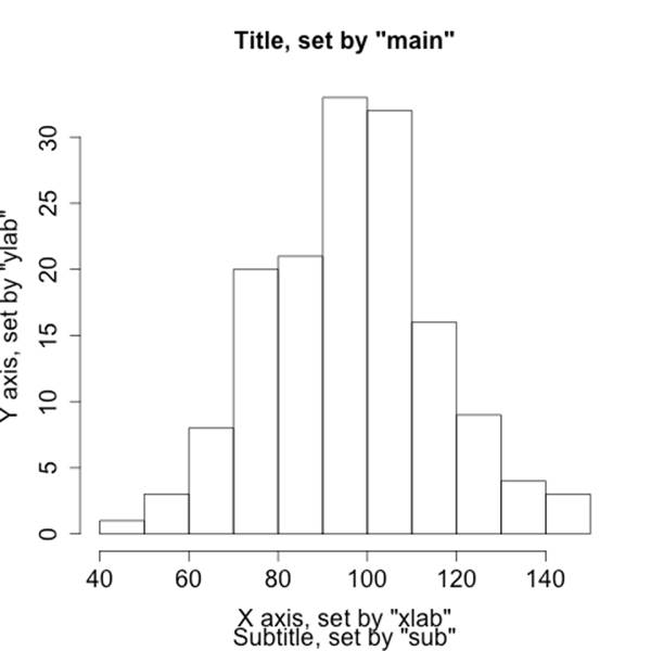
Figure 6-2. Visualizing options

Visualization options are also controlled using the par function, which provides a huge number of special options for managing axis size, point types, font choices, and the like. par takes an enormous number of options that you can read about via help(par). Table 6-3 provides some of the more important ones.

> # We're going to use par to draw a 3-columm, 2-row matrix, then fill in 3 cells

> # of the matrix with different plots using other par values

> par(mfcol=c(2,3))

> # Draw the default histogram

> hist(sample_rnorm,main='Sample Histogram')

> # Now we move to the 2nd row, center column

> par(mfg=c(2,2,2,3))

> # Change the size of the axes to half the default

> par(cex.axis=0.5)

> # Make the axes blue

> par(col.axis='blue')

> # Make the plot itself red

> par(col = 'red')

> # Now we plot as a scatter

> plot(sample_rnorm,main='Sample scatter')

> # After we've plotted this, it will automatically move to the

> # 3rd row, 1st column

> # Restore the axis size

> par(cex.axis=1.0)

> # Change the point type for a scatterplot. Use help(points) to get a list of

> # the numbers for PCH

> par(pch=24)

> plot(sample_rnorm,main='Sample Scatter with New Points')

Table 6-3. Useful par arguments

Annotating a Visualization

When drawing visualizations, I usually prefer to have some kind of model or annotation available to compare the visualization against. For example, if I’m comparing a visualization against a normal distribution, I want the appropriate normal distribution on the screen to compare it against the results of the histogram.

R provides a number of support functions for drawing text on a plot. These include lines, points, abline, polygon, and text. Unlike the high-level plot functions, these write directly to the screen without resetting the image. In this section, we will show how to use lines and text to annotate an image.

We’ll begin by generating a histogram for a common scenario: scanning traffic plus typical user traffic on a /22 (1024 host) network. The observed parameter is the number of hosts, and we assume that under normal circumstances, that value is normally distributed with a mean of 280 hosts and a standard deviation of 30. One out of every 10 events will take place during a scan. During the scan, the count of hosts observed is always 1024, as the scanner hits everyone on the network.

> # First we model typical activity using a gaussian distribution via rnorm

> normal_activity <- rnorm(300,280,30)

> # We then create a vector of attacks, where every attack is 1024 hosts

> attack_activity <- rep(1024,30)

> # We concatenate the two together; because we're focusing on the number of

> # hosts and not a time dependency, we don't care about ordering

> activity_vector<-c(normal_activity, attack_activity)

> hist(activity_vector,breaks=50,xlab='Hosts observed',\

ylab='Probability of Occurence',prob=T,main='Simulated Scan Activity')

Note the breaks and prob arguments in the histogram. breaks governs the number of bins in the histogram, which is particularly important when you’re dealing with a long-tailed distribution like this model. prob plots the histogram as a density rather than as frequency counts.

We will now fit a curve. To do so, we create a vector of x and a vector of y values for the lines function. The x values are evenly split points on the range covered by our empirical distribution, while the y values are derived using the dnorm function:

> xpoints<-seq(min(activity_vector),max(activity_vector),length=50)

> # Use dnorm to calculate the corresponding y values, given a feed

> # of x values (xpoints) and a model of a normal distribution using

> # the mean and sd from the activity vector. The value will be a poor

> # fit, as the attack skews the traffic.

> ypoints<-dnorm(xpoints,mean=mean(activity_vector),sd=sd(activity_vector))

> # Plot the histogram, which wipes the canvas clean

> hist(activity_vector,breaks=50,xlab='Hosts observed',\

ylab='Density',prob=T,main='Simulated Scan Activity')

> # Draw the fit line, using lines

> lines(xpoints,ypoints,lwd=2)

> # Draw text. The x and y value are derived from the plot.

> text(550,0.010,"This is an example of a fit")

Exporting Visualization

R visualizations are output on devices, which can be called by using a number of different functions. The default device is X11 on Unix systems, quartz on Mac OS X and win.graph on Windows. R’s help for Devices (note the case) provides a list of what’s available on the current platform.

To print R output, open an output device (such as png, jpeg, or pdf) and then write commands as normal. The results will be written to the device file until you deactivate it using dev.off(). At this point, you should call your default device again without parameters.

> # Output a histogram to the file 'histogram.png'

> png(file='histogram.png')

> hist(rnorm(200,50,20))

> dev.off()

> quartz()

Analysis: Statistical Hypothesis Testing

R is designed to provide a statistical analyst with a variety of tools for examining data. The programming features discussed so far in this chapter are a means to that end. The primary features we want to use R for are to support the construction of alarms by identifying statistically significant features (see Chapter 7 for more discussion of alarm construction).

Identifying attributes that are useful for alarms requires identifying “important” behavior, for various definitions of important. R provides an enormous suite of tools for exploring data and testing data statistically. Learning to use these tools requires an understanding of the common test statistics that R’s tools provide. The remainder of this chapter focuses on these tasks.

Hypothesis Testing

Statistical hypothesis testing is the process of evaluating a claim about the behavior of the world based on the evidence from a particular dataset. A claim might be that the data is normally distributed, or that the attacks on our network come during the morning. Hypothesis testing begins with a hypothesis that can be compared against a model and then potentially invalidated. The language of hypothesis testing is often counterintuitive because it relies on a key attribute of the sciences—science can’t prove an assertion, it can disprove that assertion or, alternatively, fail to disprove it. Consequently, hypothesis tests focus on “rejecting the null hypothesis.”

Statistical testing begins with a claim referred to as the null hypothesis (H₀). The most basic null hypothesis is that there is no relationship between the variables in a dataset. The alternative hypothesis (H₁) states the opposite of the null—that there is evidence of a relationship. The null hypothesis is tested by comparing the likelihood of the data being generated by a process modeling the null, under the assumptions made by the null.

For example, consider the process of testing a coin to determine whether it’s evenly weighted or weighted to favor one side. We test the coin by flipping it repeatedly. The null hypothesis states that the probability of landing heads is equal to the probability of landing tails: P=0.5. The alternative hypothesis states that the weighting is biased toward one side.

To determine whether the coin is weighted, we have to flip it multiple times. The question in constructing the test is how many times we have to flip the coin to make that determination. Figure 6-3 shows the breakdown of probabilities for coin flipping combinations^[7^] for one through four flips.

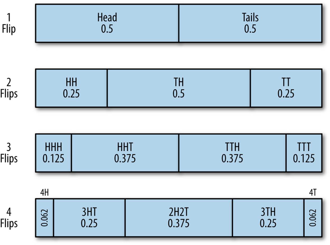
Figure 6-3. Model of coin flipping for an evenly weighted coin

The results follow the binomial distribution, which we can calculate using R’s dbinom function.^[8^]

> # Use dbinom to get the probabilities of 0 to 4 heads given that

> # there are 4 coin flips and the probability of getting heads on

> # an individual flip is 0.5

> dbinom((0:4),4,p=0.5)

[1] 0.0625 0.2500 0.3750 0.2500 0.0625

> # results are in order - so 0 heads, 1 heads, 2 heads, 3 heads, 4 heads

In order to determine if a result is significant, we need to determine the probability of the result happening by chance. In statistical testing, this is done by using a p-value. The p-value is the probability that if the null hypothesis is true, you will get a result at least as extreme as the observed results. The lower the p-value, the lower the probability that the observed result could have occurred under the null hypothesis. Conventionally, a null hypothesis is rejected when the p-value is below 0.05.

To understand the concept of extremity here, consider a binomial test with no successes and four coin flips. In R:

> binom.test(0,4,p=0.5)

Exact binomial test

data: 0 and 4

number of successes = 0, number of trials = 4, p-value = 0.125

alternative hypothesis: true probability of success is not equal to 0.5

95 percent confidence interval:

0.0000000 0.6023646

sample estimates:

probability of success

0

That p-value of 0.125 is the sum of the probabilities that a coin flip was four heads (0.0625) AND four tails (also 0.0625). The p value is, in this context “two tailed,” meaning that it accounts for both extremes. Similarly, if we account for one heads:

> binom.test(1,4,p=0.5)

Exact binomial test

data: 1 and 4

number of successes = 1, number of trials = 4, p-value = 0.625

alternative hypothesis: true probability of success is not equal to 0.5

95 percent confidence interval:

0.006309463 0.805879550

sample estimates:

probability of success

0.25

The p-value is 0.625, the sum of 0.0625 + 0.25 + 0.25 + 0.0625 (everything but the probability of 2 heads and 2 tails).

Testing Data

One of the most common tests to do with R is to test whether or not a particular dataset matches a distribution. For information security and anomaly detection, having data that follows a distribution enables us to estimate thresholds for alarms. That said, we rarely actually encounter data that can be modeled with a distribution, as discussed in Chapter 10. Determining that a phenomenon can be satisfactorily modeled with a distribution enables you to use the distribution’s characteristic functions to predict the value.

The classic example of this estimation process is the use of the mean and standard deviation to predict values of a normally distributed phenomenon. A normal distribution has a probability density function of the form:

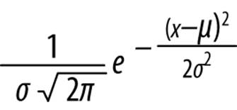
Where μ is the mean and σ is the standard deviation of the model.

If traffic can be satisfactorily modeled with a distribution, it provides us with a mathematical toolkit for estimating the probability of an occurrence happening. The chance of actually encountering a satisfactory model, as discussed in Chapter 10, is rare—when you do, it will generally be after heavily filtering the data and applying multiple heuristics to extract something suitably well behaved.

This matters because if you use the mathematics for a model without knowing if the model works, then you run the risk of building a faulty sensor. There exist, and R provides, an enormous number of different statistical tests to determine whether you can use a model. For the sake of brevity, this text focuses on two tests that provide a basic toolkit. These are:

Shapiro-Wilk (shapiro.test)

The Shapiro-Wilk test is a goodness of fit test against the normal distribution. Use this to test whether or not a sample set is normally distributed.

Kolmogorov-Smirnov (ks.test)

A goodness of fit test to use against continuous distributions such as the normal or uniform.

All of these tests operate in a similar fashion: the test function is run against a sample set and another sample set (either provided explicitly or through a function call). A test statistic describing the quality of the fit is generated, and a p-value produced.

The Shapiro-Wilk test (shapiro.test) is a normality test; the null hypothesis is that the data provided is normally distributed. See Example 6-4 for an example of running the test.

Example 6-4. Running the Shapiro-Wilk test

># Test to see whether a random normally distributed

># function passes the shapiro test

> shapiro.test(rnorm(100,100,120))

Shapiro-Wilk normality test

data: rnorm(100, 100, 120)

W = 0.9863, p-value = 0.3892

> # We will explain these numbers in a moment

> # Test to see whether a uniformly distributed function passes the shapiro test

> shapiro.test(runif(100,100,120))

Shapiro-Wilk normality test

data: runif(100, 100, 120)

W = 0.9682, p-value = 0.01605

All statistical tests produce a test statistic (W in the Shapiro-Wilk test), which is compared against its distribution under the null hypothesis. The exact value and interpretation of the statistic is test-specific, and the p-value should be used instead as a normalized interpretation of the value.

The Kolmogorov-Smirnov test (ks.test) is a simple goodness-of-fit test that is used to determine whether or not a dataset matches a particular continuous distribution such as the normal or uniform distribution. It can be used either with a function (in which case it compares the dataset provided against the function) or with two datasets (in which case it compares them to each other). See the test in action in Example 6-5.

Example 6-5. Using the KS test

> # The KS test in action; let's create two random uniform distributions

> a.set <- runif(n=100, min=10, max=20)

> b.set <- runif(n=100, min=10, max=20)

> ks.test(a.set, b.set)

Two-sample Kolmogorov-Smirnov test

data: a.set and b.set

D = 0.07, p-value = 0.9671

alternative hypothesis: two-sided

> # Now we'll compare a set against the distribution, using the function.

> # Note that I use punif to get the distribution and pass in the same

> # parameters as I would if I were calling punif on its own

> ks.test(a.set, punif, min=10, max=20)

One-sample Kolmogorov-Smirnov test

data: a.set

D = 0.0862, p-value = 0.447

alternative hypothesis: two-sided

> # I need an estimate before using the test.

> # For the uniform, I can use min and max, like I'd use mean and sd for

> # the normal

> ks.test(a.set,punif,min=min(a.set),max=max(a.set))

One-sample Kolmogorov-Smirnov test

data: a.set

D = 0.0829, p-value = 0.4984

alternative hypothesis: two-sided

> # Now one where I reject the null; I'll treat the data as if it

> # were normally distributed and estimate again

> ks.test(a.set,pnorm,mean=mean(a.set),sd=sd(a.set))

One-sample Kolmogorov-Smirnov test

data: a.set

D = 0.0909, p-value = 0.3806

alternative hypothesis: two-sided

> #Hmm, p-value's high... Because I'm not using enough samples, let's

> # do this again with 400 samples each.

> a.set<-runif(400,min=10,max=20)

> b.set<-runif(400,min=10,max=20)

> # Compare against each other

> ks.test(a.set,b.set)$p.value

[1] 0.6993742

> # Compare against the distribution

> ks.test(a.set,punif,min=min(a.set),max=max(a.set))$p.value

[1] 0.5499412

> # Compare against a different distribution

> ks.test(a.set,pnorm, mean = mean(a.set),sd=sd(a.set))$p.value

[1] 0.001640407

The KS test has weak power. The power of an experiment refers to its ability to correctly reject the null hypothesis. Tests with weak power require a larger number of samples than more powerful tests. Sample size, especially when working with security data, is a complicated issue. The majority of statistical tests come from the wet-lab world, where acquiring 60 samples can be a bit of an achievement. While it is possible for network traffic analysis to collect huge numbers of samples, the tests will start to behave wonkily with too much data; small deviations from normality will result in certain tests rejecting the data, and you can always start throwing in more data, effectively crafting the test to meet your goals.

In my experience, distribution tests are usually a poor second choice to a good visualization. Chapter 10 discusses this in more depth.

Further Reading

1. Patrick Burns, The R Inferno.

2. Richard Cotton, Learning R: A Step-by-Step Function Guide to Data Analysis (O’Reilly, 2013).

3. Russell Langley, Practical Statistics Simply Explained (Dover, 2012).

4. The R Project, An Introduction to R.

5. Larry Wasserman, All of Statistics: A Concise Course in Statistical Inference (Springer Texts in Statistics, 2004).