Mastering Autodesk Inventor 2015 and Autodesk Inventor LT 2015 (2014)

Chapter 17. Stress Analysis and Dynamic Simulation

This chapter will cover the tools of the Stress Analysis and Dynamic Simulation environments found in the Autodesk^® Inventor^® Professional software. The Stress Analysis environment allows you to perform static and modal analysis on parts and assemblies by defining component materials, loads, constraints, and contact conditions. A second type of stress analysis (referred to as frame analysis in this chapter) uses beam elements represented with a line segment that is centered in a Frame Generator member and interpolates the effects of loads on the geometry of the frame. This greatly improves the speed of the analysis.

The Dynamic Simulation environment allows you to analyze an assembly in motion by specifying loads, constraints, motion joints, velocities, acceleration, and environmental factors such as gravity and friction. These environments can be used together to determine motion loads enacted upon one component by another component at a given point in time.

In this chapter, you'll learn to

· Set up and run Stress Analysis simulations

· Set up and run Dynamic Simulations

· Export results from the Dynamic Simulation environment to the Stress Analysis environment

Introduction to Analysis

Although the terms stress analysis and finite element analysis (FEA) are often used interchangeably in conversation, it may be helpful to understand them as they relate to the tools available to you in the Inventor Stress Analysis environment. FEA is an analysis of a complex object solved by dividing that object into a mesh of smaller elements upon which manageable calculations can be run. The stress analysis done by Inventor uses this method to allow you to analyze your design, under a given set of conditions specified by you, in order to determine basic trends in regard to the specifics of your design.

Deriving an exact answer from the analysis of a model is generally reserved for an analyst with specific training, often for a more powerful set of analysis tools. With that said, you can use the Inventor simulation tools to run basic analyses to confirm design validity. This can be useful to determine design basics before going down a wrong path. Or you can use these tools to help find out, for example, whether a component or assembly is being over- or underdesigned for a given set of loads and/or vibrations. The stress analysis tools in Inventor are also useful when determining how feature size and locations will affect the integrity of the part. For instance, how close to the edge of a bracket can you move a hole? Is another brace required to prevent a sheet-metal face from “pillow casing” because of a pressure load? These tools are ideal for questions of this nature and can significantly reduce the number of physical prototypes required to prove a final design.

Dynamic Simulation allows you to set the components of your model in motion to verify how those parts interact with one another and to determine the force enacted on one component (or group of components) by another component (or group of components). The Dynamic Simulation environment allows you to define the way parts relate to one another and how the forces present create motion in the context of a timeline. From the simulation, you can determine how and when parts interact as well as the amount of force present for any point in time. For example, you might use these tools to simulate a force applied to a shaft used to turn a lever, which in turn contacts a catch stop, where the goal is to determine the maximum force present throughout the entire sequence. Once this maximum force is determined, it can be applied to the shaft as loads in a stress analysis study.

Autodesk Inventor Simulation Tutorials

If you have Inventor Professional installed, you can find a number of tutorials for the simulation tools by visiting http://wikihelp.autodesk.com. Once the tutorial files are downloaded, you'll need to point Inventor to the files by setting the project search path to tutorial_files. To do so, follow these steps:

1. In Inventor, close any open files.

2. From the Get Started tab, click the Projects button.

3. In the Projects dialog box, select tutorial_files from the list.

4. Click the Apply button at the bottom of the Projects dialog box.

5. Note the check mark next to tutorial_files in the list, denoting that it is the active project, and then click Done to close the Projects dialog box.

Now you can return to the Wiki Tutorials site and follow along.

Conducting Stress Analysis Simulations

You can simulate a stress situation on your design to determine the effects of various load and constraint scenarios to determine areas of weakness, better design alternatives, how much a part is over- or underbuilt, to what extent a design change will impact a design, and so on. Using parametric studies, you can determine a combination of these elements to see how multiple changes impact a design at the same time. For more information on this topic, refer to the section “Conducting Parameter Studies” later in this chapter. This is an important task because understanding the basic tools and workflow is the first step to setting up effective simulations.

The basic stress analysis workflow is as follows:

1. Enter the Stress Analysis environment (on the Environments tab, select Stress Analysis).

2. Create a simulation.

3. Specify the type of simulation you want to conduct (for instance, when working with assemblies, you may want to use an alternate view, positional, or level of detail representation).

4. Specify the materials for the components.

5. Specify the load types, locations, and amounts.

6. Specify the support types and locations.

7. For assemblies, gather and refine contact between components.

8. Generate a mesh.

9. Run the simulation.

10.Interpret the results.

To aid you in the process of learning how to conduct a stress analysis study, Autodesk has built in the Simulation Guide.

Simulation Guide

You can find the Simulation Guide toward the right end of the Stress Analysis tab once you have started to construct a simulation. To access the Simulation Guide, click the Guide button, and the Simulation Guide panel will appear.

This tool was built with two types of users in mind: the novice who is looking for an understanding of the process of conducting a simulation, and the intermediate user who has been using an FEA tool in the past and is looking for additional advice on using the Inventor toolset or seeking to improve their knowledge.

The tool can be launched before you begin a simulation, or if you've already started setting up a simulation, it will open to the next appropriate step to offer guidance. To help in selecting load and constraint types, the guide contains a series of hyperlinks that will step you through various options on how the component or assembly is constructed and how it moves or is supported. It will even check with you to see whether there are features that may not influence the result of the analysis but may add unnecessary time to the process.

Static Stress vs. Modal Analysis

You can perform static and modal stress analysis on parts and assemblies in the Stress Analysis environment. To enter this environment, click the Stress Analysis button on the Environments tab. Once in the Stress Analysis environment, you use the Create Simulation button and specify either Static Analysis or Modal Analysis. It's important to understand the difference between static and modal analysis:

1. Static Analysis Attempts to determine the stress placed on a component by a particular set of loads and constraints. The stress is considered static because it does not vary due to time or temperature. You can import motion loads determined from the Dynamic Simulation environment to analyze the stress at any given time step for moving parts.

2. Modal Analysis Attempts to determine the dynamic behavior of a model in terms of its modes of vibration. An example would be trying to determine whether the vibration generated by a running motor would create significant disturbance to a sensitive mechanism within the design.

Simplifying Your Model

When working with assemblies, you should exclude parts that are not affected by the simulation or do not add to its results in order to simplify the simulation and reduce the time required to run it. Excluding small parts such as fasteners, whose functionality is replicated by simulation constraints or forces, is also recommended. You can do this by expanding the assembly browser node, right-clicking the part to be excluded, and then selecting Exclude From Simulation.

When working with a part file in the simulation environment, you can suppress small features that are irrelevant to stress concentrations, such as outer fillets and chamfers. These “finish” features typically only complicate the mesh needed for the simulation and add overhead to the analysis. Other features that are typically excluded from simulations are small holes with diameters of less than 1/100th the length of the part, embossed or engraved text, and other aesthetic features. Excluding features of these types can have a significant impact on the meshing process and the simulation's run time. Figure 17.1 shows the exclusion of features from a part file on the left and the exclusion of parts from an assembly on the right. Using the appropriate selection filter, you can select features and parts to exclude in the design window using typical right-click context menu behavior while in the assembly.

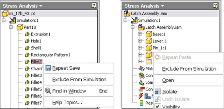
Figure 17.1 The Exclude features for a simulation

Specifying Materials

To specify the material of each part in a simulation, use the Assign button on the Material panel of the Stress Analysis tab. Material properties must be fully defined in order for the material to be used for the simulation. Materials with incomplete information are marked with an icon. Figure 17.2 shows the Assign button used to access the Assign Materials dialog box as well as the icon indicating that incomplete materials have been specified.

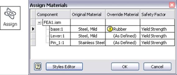
Figure 17.2 Assigning materials

You can specify the original material for each component or specify an override (per simulation) from the Material Library. To change the original material of the part file while in the Stress Analysis environment, click the Inventor button, select iProperties, and then select the Physical tab. You can use the Styles Editor button in the Assign Materials dialog box to step into the Style And Standard Editor to edit, add, or just review the properties of any material style. You can find the physical characteristics of a given material from a number of resources on the Internet, such as www.matweb.com.

It is assumed that materials are constant, meaning there is no change because of time or temperature to the structural properties of the material. All materials are assumed to be homogenous, with no change in properties throughout the volume of the part. And it is also assumed that stress is directly proportional to strain for all materials.

By default, the browser will display the names of components with overridden materials under the material name. You can also display all materials assigned to components by right-clicking the Material category in the browser and then selecting All Materials from the context menu.

Applying Simulation Constraints

Constraints added in the simulation limit the movement or displacement of the model for the purposes of the simulation. To constrain a model for static simulations, you should remove all free translational and rotational movements. You should also strive to neither over- nor underconstrain your model because both can impact the simulation results.

You can create all the constraint types by clicking the constraint tool buttons on the Constraints panel of the Stress Analysis tab, shown in Figure 17.3.

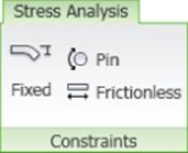
Figure 17.3 The simulation constraint tools

These are the types of simulation constraints available:

1. Fixed Constraints These remove all translational degrees of freedom and can be applied to faces, edges, or vertices, typically to simulate a part that is bonded or welded to another component. You can click the button to specify the Use Vector Components option and free the component in a given vector plane. Fixed constraints can also be used to specify a known displacement of a component to determine the force required to create the displacement.

2. Frictionless Constraints Use these constraints to prevent the selected surface from deforming or moving in a direction normal to it. You can also use frictionless constraints to simulate linear bearings and slides. Because most surface-to-surface situations are not entirely frictionless, you can expect the simulation to return more moderate results. If friction is considerable, it can be compensated for in the Dynamic Simulation environment, and the results can be imported into the Stress Analysis environment.

3. Pin Constraints These are used to apply rotational constraints on a selected cylindrical face (or faces), such as where holes are or where parts are supported by pins or bearings. Use the button to set the direction options. A pin that rotates in a hole would have only the tangential direction free, one that slides in a hole but does not rotate would have only the axial direction free, one that slides and rotates would have both the axial and tangential directions free, and so on.

Figure 17.4 shows the simulation constraint dialog boxes.

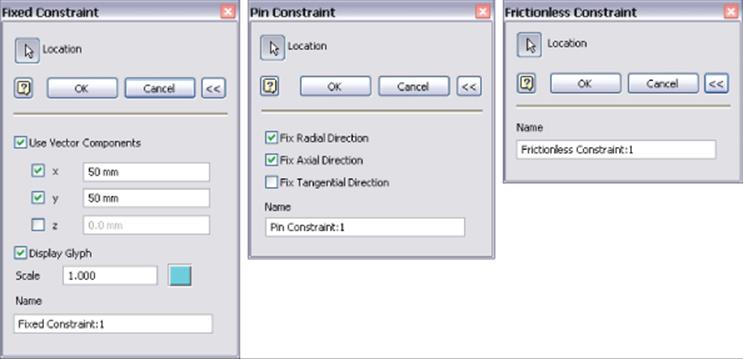
Figure 17.4 The simulation constraint dialog boxes

Applying Loads

Loads are forces applied to a part or assembly resulting in stress, deformation, and displacement in components. A key to applying loads is being able to predict or visualize how parts will respond to loads. For simple static simulations, this is generally fairly straightforward, but for more complex designs where one component exerts a force on another, which exerts a force on yet another, loads will likely need to be determined through the use of the Dynamic Simulation tools, as discussed later in this chapter.

You can access all the load types from the Loads panel of the Stress Analysis tab, as shown in Figure 17.5.

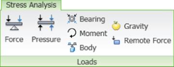
Figure 17.5 The load tools

These are the types of load available:

1. Force This is specified in newtons (N) or pounds-force (lbf or lbforce). Forces can be applied by selecting a single face, edge, or vertex (or a set of faces, edges, or vertices) for the location. Selection sets must be of the same type, meaning that once you select a face, you can add faces to the selection set but not edges or vertices. The force direction can be specified by selecting an edge or face and then changed using the Flip Direction button. Direction is automatically set to the normal of the face (with the force directed at that face) when a face is selected for either a location or a direction. You can avoid stress singularities by selecting faces or the location rather than edges or vertices.

2. Pressure This is specified in megapascals (MPa) or pounds per square inch (psi). Pressure can be applied only to a face or set of faces. Pressure is uniform and is applied in a direction normal to the surface at all locations. When applying loads to faces that are involved in contacts, you should use pressure instead of force.

3. Bearing These are specified in newtons (N) or pounds-force (lbf or lbforce). Bearing loads are applied only to cylindrical faces. By default, the load is along the axis of the cylinder, and the direction is radial. You can specify the direction by selecting a face or edge. These are generally used to simulate a radial load such as a roller bearing.

Loads and Constraints

Loads and constraints can be applied to the same entity as long as they are compatible. When incompatible loads and constraints exist on the same entity, such as a face fixed in the X direction while a load is applied in the same direction to the same face, the constraints will override the forces.

4. Moment These are specified in units of torque such as newton meters (N m or N*m) or pounds-force inch (lbforce in or lbf*in). Moment locations can be applied to faces only. Direction can be defined by selecting faces, straight edges, axes, and two vertices.

5. Remote Force These can be used as an alternative to applying a force load directly to a part by specifying the location in space from which the force originates. Apply Remote Force by selecting faces and specifying in N or lb.

6. Gravity These are specified in units of acceleration such as millimeter per second squared (mm/s²) or inch per second squared (in/s²). Apply gravity to a face or parallel to a selected edge. The default gravity value is set to 386.220 in/s² or 9810.000 mm/s².

7. Motion

Unlike with the other forces, there is no tool to apply motion loads in the Stress Analysis environment; instead, these are created from reaction forces determined from the Dynamic Simulation environment using the Export To FEA tool for a component per specified time step(s). Once they are created, you can use motion loads by one of the following methods: For a new simulation, click the Create Simulation button on the Stress Analysis tab. For an existing simulation, right-click the existing simulation in the browser node, and select Edit Simulation Properties.

In either case, once the Simulation Properties dialog box is open, you follow these steps:

1. In the Simulation Properties dialog box, select the Motion Loads Analysis check box.

2. Select the part from the enabled list.

3. Select the time step from the list.

4. Click the OK button.

Body

These are specified in units of acceleration such as millimeter per second squared (mm/s²) or inch per second squared (in/s²). Body loads are the forces acting on the entire volume or mass of a component, such as gravity, linear acceleration, centripetal force, andcentrifugal force. Select a planar face for linear acceleration or a cylindrical face for an axial direction. Use a body force to simulate the effect of outside forces. Only one body force per simulation is allowed.

Use the Linear tab to specify linear acceleration and the Angular tab to specify angular velocity or angular acceleration. The Angular tab has three possible results depending on what is specified and how:

· Velocity and acceleration have the same rotation axis, with an unspecified location. The solver determines the location along the axis.

· Velocity and acceleration have different rotation axes, with an unspecified location. The solver determines the location along the axis. A point is selected along the velocity rotation axis for the acceleration location.

· Velocity and acceleration have different rotation axes, with a specified location. The solver determines the location the same as when you define the point with the vector components.

Using Split to Apply Loads Accurately

When you assign bearing loads to components, you may need to split the face first in order to select just a portion of a continuous face. For instance, consider applying a load to a shaft. If you select the cylindrical face, the load might be distributed along the entire face rather than concentrated on just the area intended to be loaded. You can use a work plane to split the face. This can be useful when placing loads on flat surfaces as well. Use a sketch to divide the surface into a face appropriate to the load. You can access the Split tool in the modeling environment from the Modify panel of the Model tab.

Specifying Contact Conditions

Contacts between components are detected when the simulation is run and automatically listed in the browser under the contact node. However, you can run the Automatic Contact tool to see them before running the simulation and then modify any of the automatic contacts listed or manually add other contacts. To add contacts, click either the Automatic or Manual button on the Contacts tab, shown in Figure 17.6.

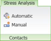
Figure 17.6 Contact tools

For contacts to be added, the faces must meet the following criteria:

· The selected faces must be within 15 degrees of parallel. This 15-degree limit is a system setting and cannot be changed.

· The distance between the selected faces cannot exceed the Tolerance setting specified in the simulation's properties. You can access the simulation's properties by right-clicking the simulation node in the browser for existing simulations, or you can specify them when you create the simulation.

Contacts are listed in the contact node in the browser and categorized per contact type. The type and components involved are set in the contact node name. Contacts are also listed under the browser node of each involved component. Modal analysis lists only the Bonded and Spring contact types, whereas all types are available for static analysis. You can change the contact type of automatic contacts by right-clicking a contact and choosing Edit Contact or by using the Ctrl or Shift key to multiselect contacts and then right-clicking and choosing Edit Contact. You can suppress contacts as well. Figure 17.7 shows the edit options.

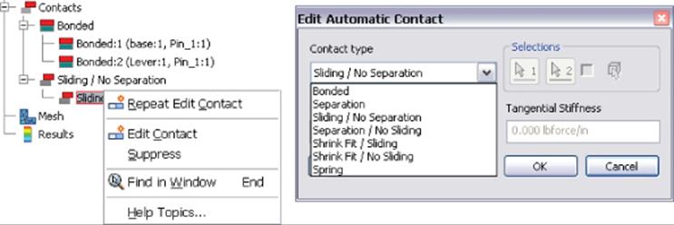
Figure 17.7 Contact edit options

These are the available contact types:

1. Bonded This creates a rigid bond between selected faces.

2. Separation This partially or fully separates selected faces while sliding.

3. Sliding/No Separation This creates a normal-to-face direction bond between selected faces while sliding under deformation.

4. Separation/No Sliding This partially or fully separates selected faces without them sliding against one another.

5. Shrink Fit/Sliding This creates conditions similar to Separation but with a negative distance between contact faces, resulting in overlapping parts at the start.

6. Shrink Fit/No Sliding This creates conditions of Separation/No Sliding but with a negative distance between contact faces, resulting in overlapping parts at the start.

7. Spring This creates equivalent springs between the two faces. You define total Normal Stiffness and/or Tangential Stiffness. The Normal Stiffness and Tangential Stiffness options are available for the Spring contact only.

You can change the contacts between two components to see how the simulation results change. Figure 17.8 shows the same simple assembly simulation with a different contact applied between the two plates. On the left, a bonded contact is used, and the results show that the vertical plate is deformed by the load and that stress is concentrated at, and distributed out from, the contact joint. On the right, a Sliding/No Separation joint is used, and the results show that the vertical plate is essentially pushed along the horizontal plate, with the stress being spread over the vertical plate and little or no concentration and no stress being distributed to the horizontal plate.

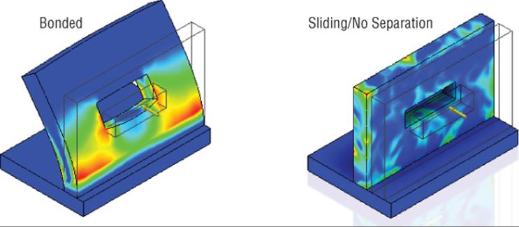
Figure 17.8 Contact comparison

Preparing Thin Bodies

Your models sometimes contain components that have thin walls compared to the overall size of the model, such as sheet metal or plastic parts. As a result of this variation, standard analysis can cause long meshing times and instabilities in the computation. To deal with this, you can use the tools on the Prepare panel to simplify thin wall bodies to be seen as surface shells.

When you use the Find Thin Bodies tool, the model is scanned and any bodies found to have a high Length/Thickness ratio are identified as potential thin bodies, and you are given the option to generate mid-surfaces for the body. Alternatively, you can use the MidSurface tool to generate mid-surfaces for bodies you know to be considered thin bodies in advance. You can also use the Offset tool to create a shell from selected faces.

Once mid-surfaces or offset shells are created, you can convert them back to solids by selecting them in the browser, right-clicking, and choosing Delete. Keep in mind that loads and constraints applied to solid bodies before preparing them as thin bodies become sick when converted to shell elements and might need to be deleted. Figure 17.9 shows the Prepare tools on the left.

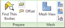
Figure 17.9 Prepare and Mesh tools

Generating a Mesh

Although you can accept the default mesh settings and run the simulation, often you will want to adjust the mesh settings to compensate for areas where a finer mesh is required. You can adjust the global mesh settings or use a local mesh control when needed. Figure 17.9 shows the Mesh tools on the right.

Mesh Settings

Use the Mesh Settings tool to change these mesh properties:

1. Average Element Size Controls the mean distance between mesh nodes. Setting Average Size to a smaller value results in a finer mesh. This setting is relative to the overall size of the model. A value from 0.100 to 0.050 is generally recommended.

2. Minimum Element Size Controls the minimum distance between mesh nodes as a fraction of the Average Size value. Increasing this will decrease the mesh element density. Decreasing this value will increase the mesh element density. This setting is sensitive, and changes typically result in dramatic changes to the mesh quality. A value from 0.100 to 0.200 is generally recommended.

3. Grading Factor Controls the ratio of adjacent mesh edges where fine and coarse mesh areas come together. The smaller the factor used, the more uniform the mesh will be. A value of 1 to 10 can be used, but a value from 1.5 to 3.0 is typically recommended.

4. Maximum Turn Angle Controls the maximum angle for meshes applied to arcs. Specifying a smaller angle results in a finer mesh on curved areas. A value between 30 and 60 degrees is typically recommended.

5. Create Curved Mesh Elements Controls the creation of meshes with curved edges and faces. If this is unselected, a less-accurate mesh is created, but performance may be better.

6. Use Part-Based Measure For Assembly Mesh This sets part mesh sizes relative to the overall dimensions of the part models. Deselecting this option sets the mesh size relative to the overall assembly dimensions. Use this option for assemblies composed of several parts of varying sizes. This setting is available only in an assembly.

Once the mesh settings have been adjusted, you can click the Mesh View button to generate the mesh initially and then toggle on the visibility of the mesh afterward. It is not required that you generate the mesh manually, because it will be done during the simulation, but doing so may allow you to identify areas of importance on the model that are not meshed to your liking and then apply a local mesh.

Local Mesh Control

You can use the Local Mesh Control button to select faces and edges that require a finer meshing than what is required for the rest of the model. This allows you to manually improve the mesh quality for small or complex faces. A browser node is created in the Mesh node for each local mesh you create. You can right-click the local mesh and select Edit Local Mesh Control to change the mesh size or change the faces or edges selected.

When mesh settings or local mesh controls have been updated, a lightning bolt icon will display in the browser to indicate that the mesh is out-of-date. You can right-click the Mesh browser node and choose Update Mesh, as shown in Figure 17.10. This figure shows a simple cube with a local mesh applied to the top face; the other faces are meshed according to the mesh settings.

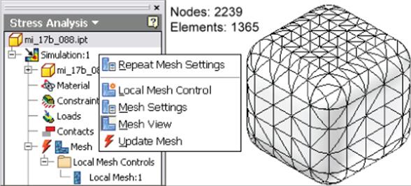
Figure 17.10 Updating a mesh

Understanding Mesh Settings

To understand the way these settings affect the mesh generated, you can use the file mi_17b_88.ipt in the Chapter 17 directory of the Mastering Inventor 2015 folder and apply a mesh to it. This file is a simple cube with rounded edges. Experiment with the options using the Mesh Settings tools. Then apply a local mesh. Exit the Stress Analysis environment, edit the model, and change the value for Extrusion1 to 30 mm (all of the dimensions of the cube are set to be the same and will update to match).

Return to the Stress Analysis environment, and update the mesh. Note that the mesh adjusts as the cube size increases, whereas the local mesh holds an absolute size. Use the Mesh Settings tool to take a look at the other settings as well. Understanding the impact of each setting on a simple part model will allow you to determine the effect of each setting on your more complex models.

Mesh Errors

When model errors prevent a mesh from being created, a mesh failure warning is displayed. Errors are reported in the Mesh progress dialog box, in the Mesh browser node, and with an error label and leader on the model in the graphics area.

An Interface Option Worth Noting

The previous sections discuss the selection of materials, application of loads, and generation of meshes. These things are categorized in the browser.

An alternative to accessing the tools from the Stress Analysis tab is to right-click these categories in the browser and select the same tools from the context menu presented.

Running the Simulation

Once you have set the material, loads, constraints, and contacts, you are ready to run the simulation. To run a simulation, click the Simulate button on the Solve panel, or right-click the Simulation node in the browser and select Simulate. The Simulate dialog box displays information about the simulation to be run and will display warning and stop errors when not all criteria are available to run. For instance, if you have forgotten to set a material type, the Simulate dialog box will stop you and tell you this. If you need to cancel a simulation in process, click the Cancel button or press the Esc key.

When a simulation becomes out-of-date because of changes to mesh settings, loads, constraints, or other design parameters, you will see a red lightning bolt next to the Results browser node. To update the simulation, simply right-click the browser node and click Simulate, or just click the Simulate button on the Solve panel again.

When working with parametric studies, it is possible to run simulations for more than one configuration at a time. You can run an Exhaustive Set or Smart Set of configurations or just run the current configuration. You can find more information on simulating configurations in the section “Conducting Parameter Studies” later in this chapter.

External Linked Files Created by Simulation Results

Be aware that by default the Results files are created and linked to your file when you run a simulation. These externally linked files can cause file-resolution problems when you move or copy simulation files or if you use Autodesk Vault. You can avoid the linked files by clicking the Stress Analysis Settings button and then activating the Solver tab. Then locate the Create OLE Link To Result Files option and uncheck the check box.

To remove links created when this check box was selected, you can go to the Tools tab and click the Links button on the Options panel. In the Document Links And Embeddings dialog box, select a link path and use the Break Link button to remove the link.

Interpreting the Results

Once a simulation is run, the Results node of the browser is populated, and the graphics area updates to show the shaded distribution of stresses. You can switch between available results types by double-clicking each type in the Results browser folder. Figure 17.11shows a typical simulation result. Note the Results folder in the browser.

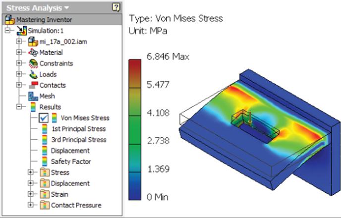
Figure 17.11 Simulation results

The Results node of the browser will display the subcategories of results, each displayed on the model by the use of color contours. The colors displayed on the model correspond to the value ranges shown in the color bar legend. Typically, areas of interest are displayed in warm colors such as red, orange, and yellow. These colors represent areas of high stress, high deformation, or a low safety factor. You can adjust the number of colors used in the color bar as well as the position and size of it by clicking the Color Bar button on the Display panel. Listed here are the result subcategories:

1. Von Mises Stress Maximum stress theory states that failure will occur when the maximum principal stress in a component reaches the value of the maximum stress at the elastic limit. This theory works to predict failure for brittle materials. However, in elastic bodies subject to three-dimensional loads, complex stresses are developed, meaning that at any point within the body there are stresses acting in various directions. The Von Mises criterion calculates whether the combining stress at a given point will cause failure. This is represented in the Results node as the Von Mises Stress, also commonly known as equivalent stress.

2. 1st Principal Stress Principal stresses are calculated by converting the model coordinates so that no shear stresses exist. The 1st principal stress is the maximum principal stress and is the value of stress that is normal to the plane in which shear stress is zero. This allows you to interpret maximum tensile stress present because of the specified load conditions.

3. 3rd Principal Stress The 3rd principal stress is the minimum principal stress, and it acts normal to the plane in which shear stress is zero. It helps you to interpret the maximum compressive stress present in the part because of the specified load conditions.

4. Displacement The displacement results show you the deformed shape of your model in a scaled representation, based on the specified load conditions. Use the displacement results to determine the location and extent to which a part will bend and how much force is needed for it to bend a given distance.

5. Safety Factor The safety factor is calculated as the yield strength of the material divided by principal stress. This shows you the areas of the model that are likely to fail under the specified load conditions. The calculated safety factor is shown on the color bar legend as the value followed by min. A safety factor of less than 1 indicates a permanent yield or failure.

6. Frequency Modes Modal results appear under the Results node in the browser as frequency modes only when a modal analysis is running. You can view the mode plots for the number of specified natural frequencies. In an unconstrained simulation, the first six modes will occur at 0 Hz, corresponding to the six standard rigid body movements.

Using the Result, Scaling, Display, and Report Tools

You can use several display tools to adjust the Results display to clearly interpret the calculated results. You can access these tools on the Result, Display, and Report panels, as shown in Figure 17.12.

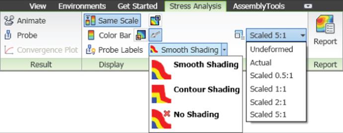
Figure 17.12 Result, Scaling, Display, and Report tools

The following list describes the Result, Scaling, Display, and Report tools available on the Display panel:

1. Same Scale Maintains the same scale while different results are viewed. This might be grayed out if no parametric table has been created.

2. Color Bar Opens the Color Bar dialog box so you can adjust the color bar display settings.

3. Probe Allows you to select the model and display results information for the selection. Right-click a label to edit or delete it.

4. Probe Labels Display Toggles the visibility of probe labels.

5. Shading Displays color changes using a blended transition when set to Smooth Shading, striated shading when using Contour Shading, and no color shading when set to No Shading.

6. Maximum Turns on and off the display of the point of maximum result, which allows you to quickly identify the maximum result on the model.

7. Minimum Turns on and off the display of the point of minimum result, which allows you to quickly identify the minimum result on the model.

8. Boundary Condition Turns on and off the display of load symbols on the part.

9. Adjust Displacement Scale Allows you to select from a preset list of displacement exaggeration scales.

10.Element Visibility Displays the mesh over the top of the result contours.

11.Animate Displacement Animates the displacement for the current result type and displacement scale.

12.Report Generates reports of analysis simulations in HTML format with PNG graphics.

Conducting Parameter Studies

Often the purpose of a stress analysis simulation is to determine how a change to a design feature will impact the part or assembly's strength. The parametric study tools allow you to make comparative evaluations based on different parameter values at the feature, part, and assembly levels. To create a parametric study, you nominate certain parameters for evaluation in the study, define the range for each parameter, specify the design constraints that you are interested in seeing for those parameters, and, finally, analyze the results of each variation.

To create a parametric study, use these steps as a guideline:

1. Set the simulation's design objective to Parametric Dimension. How you do this depends on whether you are creating a new simulation or editing an existing one. You can set the design objective to Parametric Dimension by using the Create Simulation button when creating a new simulation or by right-clicking an existing simulation in the browser and choosing Edit Simulation Properties, as shown in Figure 17.13.

2. Nominate selected parameters for use in the study by expanding the browser node for the model and then right-clicking the assembly, part, or feature node you want to use in the study and selecting Show Parameters. Figure 17.14 shows a parameter called Side_Offset being nominated.

3. Define the range for the selected parameters by following these steps:

A. Click the Parametric Table button on the Manage panel of the Stress Analysis tab.

B. Enter a parameter range in the Values column; values must be in ascending order.

C. Create a simple range by separating the minimum and maximum values with a hyphen; for instance, you can enter 70-85.

D. Specify specific values in a range by separating each value with a comma, colon, hyphen, or slash; for instance, you can enter 70, 75, 80, 85.

E. Add a colon to a range to specify the number of points included; for instance, you can enter 70-85: 4.

F. Use the slider to set the current value.

G. Right-click the parameter row and choose from the options to generate the geometry configurations. For instance, if you were to set the range of a hole position to 70, 75, 80, 85, four model configurations would be created with the hole positioned at each of those values. Figure 17.15 shows a Parametric Table configuration for the Side_Offset parameter.

4. Add design constraints to the Parametric Table by following these steps:

A. In the Design Constraints area of the Parametric Table, right-click a row and select Add Design Constraint.

B. In the Select Design Constraint dialog box, specify a results component, such as Von Mises Stress, Displacement, Safety Factor, and so on.

C. Specify the value of interest, such as Minimum or Maximum (this applies to all geometry).

D. You can modify the selection set by selecting Include or Exclude and then selecting bodies, faces, or edges on-screen. Doing so focuses the results to a specific area of interest. Figure 17.16 shows the Safety Factor design constraint being added.

5. Specify the constraint type, set limits, enter a safety factor, and review the results using the following steps:

A. In the Parametric Table dialog box, click the Constraint Type drop-down, and select from the list.

B. Enter a value in the Limit column to filter the results to the set that meets the bounding limit when you're optimizing other design constraints.

C. Enter a safety factor to specify at what extent a variable can be exceeded before causing the design constraint to fail. A comparison to the limit factored by the Safety Factor setting determines whether it meets the limit or range.

D. The Result Value column displays the value of the design constraint for the simulation. When the value is within the limit, it displays green. When the limit is exceeded, it displays red. When out of range, it displays gray, and the closest value is displayed.Figure 17.17 shows the Mass design constraint being configured.

6. When multiple parameters are added to the table, configurations can be created. These configurations can then be generated and simulated by following a few simple steps:

A. In the Parametric Table dialog box, set the parameter values to the combination you want to simulate, right-click any parameter row, and choose Simulate This Configuration.

B. To simulate all configurations, exit the Parametric Table dialog box and click the Simulate button on the Solve panel. You can choose to run an exhaustive set, a smart set, or the current configuration.

C. Once the simulations have been run, you can use the slider bar in the Parametric Table dialog box for each parameter to set the combinations and observe the results.

D. The Exhaustive Set Of Configurations setting runs all possible combinations of parameter settings, whereas the Smart Set Of Configurations setting runs only those combinations of parameter settings that Inventor determines have not yet been run. Figure 17.18 shows the choices for running simulation configurations.

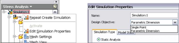
Figure 17.13 Setting a simulation to the Parametric Dimension design objective

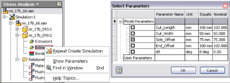
Figure 17.14 Nominating a parameter

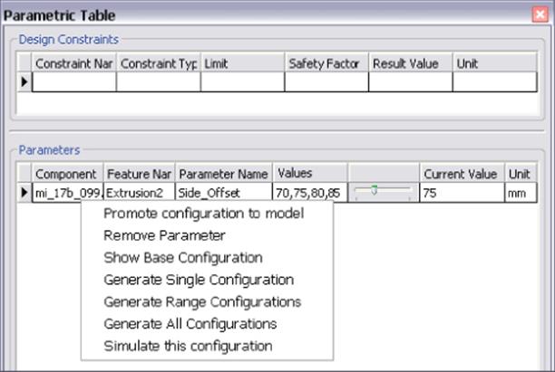
Figure 17.15 Defining a parameter range

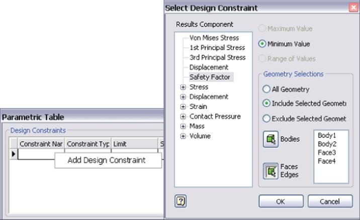
Figure 17.16 Adding a design constraint

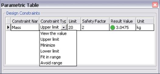
Figure 17.17 Configuring a design constraint

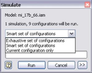
Figure 17.18 Simulation configurations

Once you determine that a given configuration satisfies your design needs using the Parametric Table dialog box, you can right-click any of the parameter rows in the table and choose Promote Configuration To Model. This will write the parameter values of the configuration to the source files.

Conducting a Frame Analysis

As you learned in Chapter 15, “Frame Generator,” having a library of predefined metal shapes can save a tremendous amount of work because you won't have to re-create standardized geometry. Frame Analysis allows you to further leverage those predefined shapes by using the known behavior of the shape under load and calculating what the loads would be along the center of a length of material rather than the surface.

The process of conducting a frame analysis is similar to performing an assembly analysis, but frames add some additional tools that allow for an even more efficient solving process. Here is the process, including some optional steps:

1. Enter the Frame Analysis environment through the Environments tab or by using the icon on the Design tab.

2. Create a simulation.

3. Specify the support types and locations.

4. Specify the load types, locations, and amounts.

5. Specify connections between beams, additional nodes, or releases (optional).

6. Run the simulation.

7. Interpret the results.

Frame Analysis Settings

You can adjust Frame Analysis settings by clicking the Frame Analysis Settings button on the Frame Analysis tab. On the General tab, you can adjust the colors, scales, and interface display. If you deselect the Use HUD In Application check box, you can use the traditional dialog box interface. By default, the Heads Up Display (HUD) interface is selected.

On the Beam Model tab, you can choose to automatically create rigid links, which allows you to adjust the model during automatic conversion. When the check box is cleared, rigid links are not created automatically during model conversion, but you can create rigid links manually later. You can also use the Trim Mitered Beam Ends option to trim overlapping ends during automatic model conversion, which simplifies the model and improves the accuracy of the simulation results.

The Solver and Diagrams tabs can be used to tweak the style of the simulation outputs and graphs ahead of time.

Frame Constraints

The concept of the constraint is the same for Frame Analysis, but the realities of how a frame is constructed can be different. Portions of the frame may be built with the ability to have one end move freely or slide along another member. This opens up the need to be able to approach things differently to assure accuracy.

You can access all the constraint types from the Constraints panel of the Frame Analysis tab, as shown in Figure 17.19.

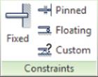
Figure 17.19 The frame constraints

These are the types of constraints available:

1. Fixed Constraint Like the Fixed constraint in FEA, it restricts all movement of the beam or node to which it is applied.

2. Pinned Constraint Applying the Pinned constraint to a beam or node will allow rotation about the selected element, but it cannot move in space.

3. Floating Constraint This constraint allows free rotation of the beam or node, but it also allows movement in one plane.

4. Custom Constraint If you need a node or beam to be able to move or rotate within a boundary or with an amount of elasticity, the Custom constraint can establish those conditions in any or all directions, including the ability for that movement to be unidirectional for one value and free in another direction.

Frame Loads

When the need to apply a mesh to a frame model is removed, it may become necessary to define the loads in a different manner. This means that there are more options for loads in frame analysis.

The three primary loads are shown in the Loads panel of the Frame Analysis tab, as shown in Figure 17.20:

1. Force This is specified in newtons (N) or pounds-force (lbf or lbforce). The value of the force can be applied to a node along the length of a beam. Once an approximate position has been selected, a dialog will appear and prompt you for the position along the beam element. The icon that appears has a series of handles that allow you to change the angle of the plane in which the force is applied and the angle to the plane of the force; if you click the arrow that represents the direction of the force, the dialog will prompt you for the magnitude of force.

2. Continuous Load This is specified in newtons (N) or pounds-force (lbf or lbforce). This force applies evenly to the entire beam segment. The settings allow you to specify End Magnitude, Direction, Offset, and Length values.

3. Moment

This is specified in units of torque such as newton meters (N m or N*m) or pounds-force per inch (lbforce in or lbf*in). A moment can be applied to a point at the end or along the beam segment with a graphical input similar to the on-screen feedback for applying a force.

There are also two types of load you can choose under Moment in a drop-down menu:

4. Axial Moment This is specified in units of torque such as newton meters (N m or N*m) or pounds-force per inch (lbforce in or lbf*in). This is a moment that can be applied along the axis of the selected beam. You can control the position of the moment along the axis, but it is automatically normal to the axis.

5. Bending Moment This is specified in units of torque such as newton meters (N m or N*m) or pounds-force per inch (lbforce in or lbf*in). A bending moment can be applied to a point at the end or along the beam segment. It is applied in the plane of the axis. You can change the angle about the axis to which it is applied.

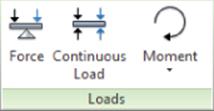
Figure 17.20 The frame loads

Connections

Working with Frame Generator by its nature involves situations where additional information may need to be added to the model for a proper simulation: conditions where there are gaps or flexibility in the model or you want to add additional nodes.

The tools for adding additional information are located in the Connections panel of the Frame Analysis tab, as shown in Figure 17.21:

1. Release This connection can be applied to a beam adjacent to another loaded beam. You can control the flexibility between the beams. The resistance to the movement can be controlled in the primary planes and around the axes using either a specific force or a partial stiffness coefficient.

2. Custom Node You can add nodes along the beam to represent where contact will be made or to shortcut the loading process.

3. Rigid Link If you have a machined or cast part built into your design, the Frame Analysis tool may not properly account for a rigid element between two points that appears to be free in the Frame Generator model. The Rigid Link tool allows you to select a parent node and have a child node maintain its position to it through the simulation.

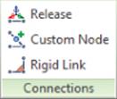
Figure 17.21 The Frame constraints

Results

People doing Frame Analysis need to understand what is happening to the model along the length of a beam. In an FEA model, this is easy to visualize, and the coloration of the beam element also helps. Over time, methods for diagramming a beam have been developed, and to offer a familiar way to understand the results of the simulation, diagramming tools have been added to the Frame Analysis environment.

These tools are located in the Result panel of the Frame Analysis tab, as shown in Figure 17.22:

1. Beam Detail This tool launches a dialog that allows you to see the basic results on the right and diagrams of the specific results for the selected beam on the left.

2. Animate Results can be animated and recorded in order to observe the displacement or stress build up over a sequence of images.

3. Probe Once a simulation is run, result values for specific points on the model can be visualized using the Probe tool. The Probe Labels button controls the visibility of probe results.

4. Diagram Selecting this tool opens a dialog where you can request various results to be displayed on the model.

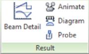
Figure 17.22 Diagramming tools

Additional tools in the Display panel will place beam and node labels in the design window (rather than highlighting them in the browser) so you can more easily understand where these elements are.

For static stress analysis, the tools offered for parts, assemblies, and frames will offer you a great opportunity to better know the effects of changes to your designs.

Considering Every Load Scenario

An engineer was involved in a redesign of an equipment accessory that had unfortunately failed in the field. The problem originated from two sources. One was the use of an incorrect material that offered too much flexibility under a particular load condition.

However, the second dynamic of this failure stemmed from the way the design was actually used in the field. During the design process, the considerations were mostly focused on how the mechanism would be operated during installation and how it would hold up under its highest load during use. Both were valid design considerations, but neither predicted the ultimate failure of the design.

As it turned out, it was the way these accessories were uninstalled that led to their high rate of failure. Not having anticipated this part of the way the product was used, the design team had no means to understand the unique torque loads that would ultimately make a good design fail. In the end, a slight modification to the design and the use of a different material type resolved the issue, but not before many dollars were wasted purchasing components that ultimately could not be used.

Keep this in mind as you create simulations, and remember that the results you generate can be only as good as the assumptions you make. Simulating every loading situation your design might encounter will expose these things before the first part is made or purchased.

Conducting Dynamic Simulations

Dynamic simulation is useful during the prototyping stages of design to test the function of interacting parts and for use in failure analysis where interacting parts enact stresses upon one another. When creating a dynamic simulation, you should follow the basic workflow listed here:

1. Define joints to establish component relationships.

2. Define environmental constraints such as gravity, forces, imposed motions, joint friction, and joint torque.

3. Run the simulation.

4. Analyze the output graph to determine maximum or minimum stress at a given time step, maximum or minimum velocities, and so on.

5. Export the results to the Stress Analysis environment for motion stress analysis simulation.

To access the Dynamic Simulation tools, first open the assembly in which you want to create the simulation and then click the Dynamic Simulation button on the Environments tab.

Working with Joints

In the Dynamic Simulation environment, joints are used to define the way that components can move relative to one another. Although you might at first associate joints with assembly relationships such as constraints, joints and constraints are actually two separate concepts. In the assembly environment, all components are assumed to have six degrees of free motion until grounded or constrained in such a way that some or all of these degrees of freedom (DOF) are removed. Standard joints approach the issue of DOF from the opposite end. In the Dynamic Simulation environment, all components are assumed to have zero DOF until joints are applied to add free motion. You can then add special joint types manually to restrict degrees of freedom.

Understanding the difference between assembly relationships and joints is important when working with joints. However, if you have a properly constrained model, much of the joint creation can be automated by setting the Simulation Settings option to Automatically Convert Constraints To Standard Joints. You can do this by clicking the Simulation Settings button on the Dynamic Simulation tab. Figure 17.23 shows the Automatically Convert Constraints To Standard Joints option.

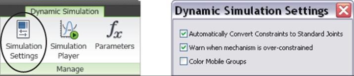
Figure 17.23 Automatic constraint-to-joint conversion

When the Convert Constraints option is on, any assembly relationships that are changed will automatically update and be converted to a standard joint when possible. You can apply relationships while in the Dynamic Simulation environment by switching to the Assemble tab. When joints are built automatically from assembly relationships, you can retain them in the model when the translator is turned off. This allows you to customize the standard joints built from relationships and author new standard joints, without starting from scratch.

When the Convert Constraints option is off, you can use the Convert Constraints button to manually convert assembly relationships. To convert constraints manually, you must have the automatic Convert Constraints option turned off and the Convert Assembly Constraint button enabled. Using the Convert Assembly Constraint tool, you simply select the parts to which you want to apply a joint, and the Assembly constraints that exist between the two will appear in the dialog box. You can deselect one or more of the constraints to apply a less-restrictive joint solution. Figure 17.24 shows the different results achieved by selecting or deselecting the relationships that exist on a shaft and handle.

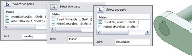
Figure 17.24 Manual constraint-to-joint conversion

In addition to the automatic joint creation, you can (and most often need to) apply joints to your model manually. You can access the joint tool by clicking the Insert Joint button. When you do so, the Insert Joint dialog box offers a drop-down with all the joint types listed. Alternatively, you can click the Display Joints Table button next to the drop-down to display the five joint categories as buttons in the top of the table. Clicking a category button shows the available joint types for that category. Figure 17.25 shows the joint categories.

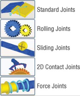
Figure 17.25 Joint categories

Standard Joints

Standard joints are created by converting assembly relationships to joints, either automatically or manually. Only one type of standard joint, called Spatial, is listed in the Display Joints table when the option to automatically create constraints is on. Here is a list of all the standard joints:

1. Revolution Joints Used to create a rotational relationship between cylindrical faces and axes of two components.

2. Prismatic Joints Used to constrain the edge of one component to the edge of another.

3. Cylindrical Joints Used to constrain the axis of one cylindrical component to the axis of another, thereby allowing the second component to slide along the axis of the first.

4. Spherical Joints Used to create ball-and-socket joints between two components.

5. Planar Joints Used to constrain the planar face of one component to the planar face of another. The first component is the motionless component, and the second is allowed to move along the face of the first.

6. Point-Line Joints Used to constrain the center point of a sphere to the axis of a cylinder or a point on another component.

7. Line-Plane Joints Used to constrain a planar face of one component to a point on another.

8. Point-Plane Joints Used to constrain the point of one component to the planar face of another.

9. Spatial Joints Used to create a relationship between two components where all six degrees of freedom are allowed without causing errors of redundancy in the simulation.

10.Welding Joints Used to create a relationship between two components so there are no degrees of freedom between them and they are considered a single body in the simulation.

Rolling Joints

Ten types of rolling joints are available. Rolling joints are used to restrict degrees of freedom. Here is a list of the rolling joint types:

1. Rolling Cylinder On Plane Joints Used to constrain a rotating cylindrical face to a 2D planar face. The relative motion between the two selected components is required to be 2D. A basic, continuous cylindrical face is required for this joint type.

2. Rolling Cylinder On Cylinder Joints Used to constrain one rotating cylindrical face to another rotating cylindrical face. The relative motion between the two selected components is required to be 2D. A basic, continuous, cylindrical face is required for this joint type.

3. Rolling Cylinder In Cylinder Joints Used to constrain one rotating cylindrical face to the inside of another rotating cylindrical face. The relative motion between the two selected components is required to be 2D. A basic, continuous, cylindrical face is required for this joint type.

Gears and Rolling Joints

If you have created a gear using the design accelerator, you will find a basic surface cylinder present in the part model. To make the surface available for use in the creation of rolling joints, you can edit the part and set the surface to be visible.

4. Rolling Cylinder Curve Joints Used to constrain a rotating cylindrical face to maintain contact with a curved face such as a cam. The relative motion between the two selected components is required to be 2D.

5. Belt Joints Used to constrain a belt component to two cylindrical components that rotate. Faces, edges, and sketches can be selected.

6. Rolling Cone On Plane Joints Used to constrain a rotating conical face to a 2D planar face. Faces, edges, and sketches can be selected.

7. Rolling Cone On Cone Joints Used to constrain a rotating conical face to another rotating conical face. Faces, edges, and sketches can be selected.

8. Rolling Cone In Cone Joints Used to constrain a rotating conical face to the inside face of a component that is not rotating. Faces, edges, and sketches can be selected.

9. Screw Joints Used to constrain components that screw together by specifying a thread pitch to define the travel per rotation. Faces, edges, and sketches can be selected.

10.Worm Gear Joints Used to constrain a component to a helical gear by specifying a thread pitch to define the travel per rotation. Faces, edges, and sketches can be selected.

Sliding Joints

The five joint types in the sliding category are used to restrict degrees of freedom between the two components selected. In all five, the relative motion between the two selected components is required to be 2D. Here are the five types of sliding joints:

1. Sliding Cylinder On Plane Joints Used to constrain a cylindrical face to a 2D planar face so that it will slide along the plane without rotating

2. Sliding Cylinder On Cylinder Joints Used to constrain a cylindrical face to slide on another cylindrical face

3. Sliding Cylinder In Cylinder Joints Used to constrain a cylindrical face to slide inside another cylindrical face

4. Sliding Cylinder Curve Joints Used to constrain a cylindrical face to slide on a curved face such as a cam

5. Sliding Point Curve Joints Used to constrain a point on the second component to slide along a curve defined by the selected face, edge, or sketch on the first component

2D Contact Joints

There is only one joint type in this category, and it is used to restrict degrees of freedom:

1. 2D Contact Joints Creates contact between curves on two selected components. Curves can be faces, edges, or sketches, but the relative motion between the selections must be planar. The contact is not required to be permanent for this joint type.

3D Contact Joints

3D contact joints create an action or reaction force when applied. This category consists of just two joint types:

1. Spring/Damper/Jack Joints These create joints for resisting forces, shock absorption, and lift jacking forces.

2. 3D Contact Joints These detect the contact and interference between all the surfaces of two selected parts. Subassemblies are not considered in this joint type.

More on Working with Joints

When components are assigned joints, either manually or automatically, they are grouped according to the results of the joints in the browser. For instance, if components are fully constrained to one another in the assembly, they will be assigned a weld joint and listed in the browser as a welded group. If one of those components is grounded, the welded group will be listed in the Grounded folder in the browser. If one of them is used in a motion joint, it will be listed in the Mobile Groups folder. Figure 17.26 shows an assembly with two welded groups present. One is listed under Grounded, and the other is listed under Mobile Groups. You'll notice that both are used in the joint called Revolution:2.

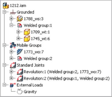
Figure 17.26 Browser grouping

Here are some points to remember when creating joints:

· The Joint Table displays a pictorial representation for each joint type to assist you with determining which to use.

· Assembly relationships are not converted to joints in a one-to-one fashion; instead, joints are often created by combining assembly relationships. For instance, a Mate and two Flush constraints between two parts might be converted to a weld joint.

· Dynamic simulation performance is affected by the number of joints present. If you are simulating a particular set of components in a large assembly, it might be beneficial to manually weld most of the components and consider motion only for the set you need.

· When placing a joint, you are often required to align the z-axis of the joint on both components. Failing to do so will prompt a warning.

· If you have the option to automatically convert the assembly relationships selected, any assembly relationship you place in the Dynamic Simulation environment will automatically be converted to a standard joint.

When placing joints, you should keep an eye on the coordinate triad and ensure that the arrows align when required. Figure 17.27 shows the use of the flip arrow to align the z-axis.

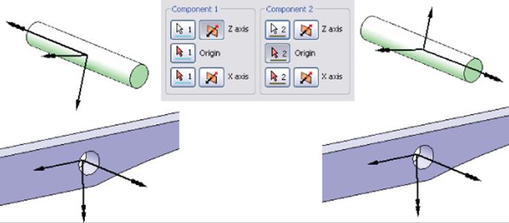
Figure 17.27 Aligning component axes

To more easily review the joints that you've placed, you can select components in the browser or the design window and joints associated with them will be highlighted in the browser.

Working with Redundancy

In the Dynamic Simulation environment, joints are said to contain redundancy when they are overconstrained or have too many unknowns to solve. When redundancy occurs in a joint, Inventor prompts you to use the Repair Redundancy tool to repair the joint. In most cases, this tool suggests one or more solutions. Figure 17.28 shows a link assembly that has a redundancy in joint 4, the cylindrical joint. To resolve this, the Mechanism Status tool is selected.

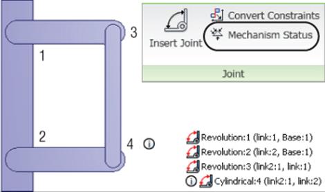
Figure 17.28 Using the Mechanism Status tool to resolve redundant joints

In the Mechanism Status And Redundancies dialog box, you can use the button to expand the options for resolving a redundancy. Typically, a new joint type is suggested for the redundant joint. Often you can expand the drop-down and select from a list of possible alternatives, as shown in Figure 17.29. This dialog can also be shown while the simulation is running.

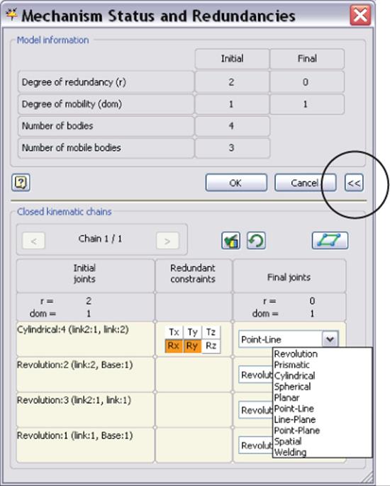
Figure 17.29 Resolving a redundant joint

Also listed in the Mechanism Status and Redundancies dialog box are the redundant constraints. Tx, Ty, and Tz are the translational (linear) constraints, and Rx, Ry, and Rz are the rotational constraints. In Figure 17.29, the cylindrical joint shows that the Rotational X (Rx) and Rotational Y (Ry) are redundant.

Working with Environmental Constraints

Once joints are applied to the model, it is often necessary to apply environmental constraints to make the joints perform more realistically or to set the simulation up more efficiently. For example, if you apply a prismatic joint between a rail and a linear bearing pad, a certain amount of friction would be anticipated, so you would modify the joint and apply a dry friction coefficient value. You might also want to create an imposed spring to emulate a spring cushion in the slide channel, or set the start position of the slide for the simulation. And then you might want to apply an imposed motion on the joint so that it moves during the simulation as expected. All of this can be done by right-clicking the joint and choosing Properties. When an environmental constraint for a particular joint is added, the constraint is marked with a green number sign next to it in the browser, as shown in Figure 17.30.

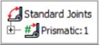
Figure 17.30 A joint with an environmental : constraint set

Modifying the Initial Position

Often you will want to change the initial position of a component involved in a joint so that the simulation will run differently from the way it is constrained. For instance, the rail and bearing pad example might be constrained so that the bearing is in the start position, but for the purposes of reducing the time of the simulation, it needs to run only from the middle of the cycle to the end. Setting the initial position allows this. To adjust the initial position of a joint, follow these steps:

1. Right-click the joint in the browser and select Properties.

2. Select the appropriate DOF tab. Depending on the joint, there may be multiple DOFs.

3. Click the Edit Initial Conditions button.

4. Enter a new position value in the input box.

Here are some additional options that may apply, depending on the simulation and results you are trying to achieve:

· Select Locked so that the joint cannot be modified in the simulation.

· Deselect the Velocity check box to manually set the initial velocity of this degree of freedom or leave it selected to allow the software to automatically compute the initial velocity. I recommend you leave this set at Computed and impose a velocity using the Impose motion option (covered in the coming pages).

· Set the initial minimum or maximum bounds values for the degree of freedom, if desired. Value sets the boundary for the force or torque of this DOF, Stiffness sets the stiffness of this DOF, and Damping sets the damping boundary for this DOF.

Joint Torques

Joint torques can be set to control damping and friction and also to impose a spring cushion. Depending on the simulation, you can often apply these things to a few key joints and have other dependent joints react off them. Of course, this depends on the mechanism and the simulation. To adjust a joint for these things, follow these steps:

1. Right-click the joint in the browser and select Properties.

2. Select the appropriate DOF tab (depending on the joint, there may be several).

3. Click the Edit Joint Torque button (the appearance of this button varies between rotational and translational joints).

4. Select the Enable Joint Torque check box.

5. Right-click an input box and choose the input type required. Use Constant Value if the value does not change over time, or use the Input Grapher to enter a graduated input.

Figure 17.31 shows the Joint Torque properties for a prismatic joint.

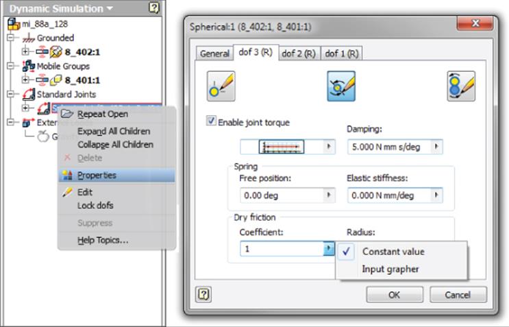
Figure 17.31 Adding friction and damping to a joint

The range of inputs for Damping, Elastic Stiffness, and Friction are listed here:

· Damping is proportional to the velocity of the DOF.

· Free Position sets the position at which an imposed spring exerts no force.

· Elastic Stiffness sets the imposed spring stiffness.

· Friction is added as a coefficient between 0 and 2.

Imposed Motion

Although motion can be created by applying external forces where it is important, often an imposed motion on a joint is desired to allow control of the timing and position of components not involved in an external force. For instance, in the rail and bearing pad example, the bearing might need to slide out of the way of another component that is being driven by an external force. Setting the imposed motion in the joint properties allows this to happen without the need to apply an external force on the bearing pad. To adjust a joint to include an imposed motion, follow these steps:

1. Right-click the joint in the browser and select Properties.

2. Select the appropriate DOF tab (depending on the joint, there may be multiples).

3. Click the Edit Imposed Motion button.

4. Select the Enable Imposed Motion check box.

5. Select a Driving motion parameter type and enter a value. The parameter types are as follows:

Position Imposes a motion to a specified position, typically specified using the Input Grapher to set the position relative to a time step (for example, move 100 cm over 10 seconds).

Velocity Imposes a motion at a specified velocity. Use constant input or use the Input Grapher to enter a variable velocity to account for startup times and so on.

Acceleration Imposes a motion as a specified acceleration. Use constant input or use the Input Grapher to enter a variable acceleration.

Using the Input Grapher

The Input Grapher is available in a number of input boxes used throughout the Dynamic Simulation environment. When an input is set to use the Input Grapher, a Graph button is present in the input box. If no Graph button is present, you can right-click in the input box and select Input Grapher from the context menu. To open the Input Grapher, simply click the Graph button.

Typically, the Input Grapher is used to specify a value that varies over time. In Figure 17.32, a velocity is being imposed on a joint starting at 0 in/s and coming up to 100 in/s in the first 10 seconds, at which time it levels off for the next 10 seconds before returning to 0 in/s at 30 seconds. The user has right-clicked in the graph to add a control point.

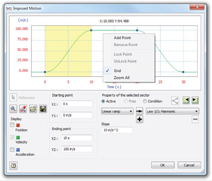
Figure 17.32 Adding a velocity curve with the Input Grapher

Each portion of the graph between points is selectable as a sector by clicking the graph. In Figure 17.32, the first sector is selected and is shaded. When a sector is selected, the inputs in the bottom half of the Input Grapher dialog box are specific to that sector. You can edit the sector's start point and endpoint as well as the law applied to that specific sector.

You can modify the input graph by changing the x-axis variable, the laws applied, the freeing sector condition, and more. The following sections briefly describe these graph input variables.

Input References

By default, Time is the x-axis variable for the curve graph in the Input Grapher. In many inputs, you can specify a different x-axis reference. Clicking the Reference button displays all variables available to be used as x-axis variables in the curve graph. Imposed motions cannot use x-axis references other than Time. Figure 17.33 shows a curve graph being set to call Velocity as the x-axis of the curve.

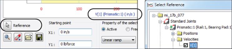
Figure 17.33 Setting the Input Grapher to use Velocity rather : than Time

Laws

To define each sector of a curve, you can assign mathematical functions, or laws. These laws can be applied individually or in combination as needed to fully define the sector curve. To assign a sector a specific law, select the law from the list in the drop-down, and then use the arrow button to apply the law. Use the plus button to add laws to the sector, and use the minus button to remove laws from the sector. Here is a list of the available laws:

· Linear Ramp

· Cubic Ramp

· Cycloid

· Sine

· Polynomial

· Harmonic

· Modified Sine

· Modified Trapezoid

· Spline

· Formula

Freeing and Application Conditions

Each sector can be set to Active, Free, or Condition. Active indicates that the sector has no conditions. Free indicates that the sector has no values defined. Condition indicates that one or more conditions have been assigned to the sector.

To create a condition, click the Condition radio button. By default, the Freeing Conditions dialog box appears. To edit or add a condition, click the Define Conditions button and then click the Variable, Equal, or Value links to set those options. Use the plus and minus signs to add or remove conditions. Figure 17.34 shows a condition being added.

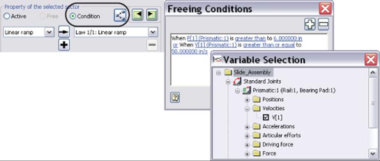
Figure 17.34 Adding conditions

More Functions

The Input Grapher has a few functions that might not be apparent but are useful to know about when you're setting up and using it:

· The bottom display is dependent on what is selected in the graph. Selecting a point gives inputs for just that point, selecting a sector gives sector options, and clicking in the graph outside all sectors gives Out Of Definition options that are used to describe the part of the curve on the left or right of the first and last points.

· Using the wheel button on your mouse, you can pan and zoom in the graph. This can be helpful when dealing with sectors that are dramatically different in scale. You can also use the Zoom button in the Input Grapher dialog box.

· Curve definitions can be saved and loaded using the Save Curve and Load Curve buttons.

External Forces

To set a component in motion, you can apply an imposed motion on the joint or apply an external force on the component itself. External forces consist of loads and gravity. External forces can be used to initiate, complement, or resist movement. For instance, in the rail and bearing pad example, if the bearing traveled past a catch stop mechanism designed to prevent back travel, you might apply an external force on the bearing pad at that position to ensure that it can overcome a maximum resistance. External forces are often used just to set the simulation in motion as well. Loads and gravity are further defined here.

Loads

You can apply as many force and torque loads as required and manage them from the External Loads browser node, where all force and torque loads are listed once created. To apply external load forces, click the Force or Torque button on the Load panel, and set the location, direction, magnitude, and so on, as described here:

1. Location For the Location setting, a vertex must be selected. You can select a vertex, circular edge, sketch point, work point, and so on.

2. Direction For the Direction setting, select an edge or face, and then use the Flip button to change it if needed.

3. Magnitude Enter the Magnitude setting as a constant, or select Input Grapher.

4. Fixed and Associative Load Buttons Use the Fixed and Associative load buttons to designate the load direction method. Fixed sets the load to be constant to the direction in which it is defined. Associative sets the direction to follow the component as it moves during the simulation. For instance, if an Associative direction is established using the edge of a hinge, the direction will stay aligned to that edge as the hinge swings.

5. The button Use the button to set the vector components as required.

6. Display Check Box Set the Display check box to see the Force or Torque arrow and then set the scale and color of the arrow.

Gravity

You can define the gravity for the entire simulation by expanding the External Load node in the browser, right-clicking the Gravity button, and choosing Define Gravity. A default value of 386.220 in/s² or 9810.000 mm/s² is supplied, but you can edit this to any value required. To define gravity, you simply select an object face or edge and then use the Flip button to set the direction. You should choose static components to define gravity.

Running a Simulation

Once the model is defined with joints, loads, and environmental constraints, you are ready to run the simulation. Running the simulation involves two primary controls: the Simulation Player and the Output Grapher. The tools are generally used together.

Simulation Player

You use the Simulation Player to run and stop the simulation. The Simulation Player is displayed by default but can be toggled on and off using the Simulation Player button on the Manage panel of the Dynamic Simulation tab. Figure 17.35 shows the Simulation Player options, and Table 17.1 provides a description of each.

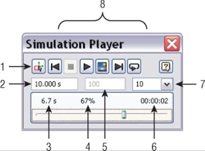
Figure 17.35 The Simulation Player

Table 17.1 Simulation Player options

The Output Grapher

You can access the Output Grapher during or after running a simulation to view and use the data collected during the simulation. Data can be exported to Microsoft Excel or marked for use in the Stress Analysis environment. You can also export the results as an IAA (*.iaa) file and import the file into another simulation for comparison of the graph results.

Once the curve type is selected, you can examine the time steps to see the value for each step. Figure 17.36 shows an acceleration curve displayed in the Output Grapher. The time step for six seconds is selected (1) and is marked in the graph area with a vertical line (2). You can click in the graph area to select a time stamp or select it from the top pane. You can also use the arrow keys on the keyboard to advance through each step.

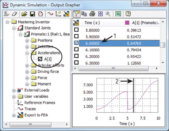
Figure 17.36 An acceleration curve in the Output Grapher

You can use the Save Simulation button to save a simulation result before making changes and then use the Import Simulation button to bring it back in once the modified simulation has been run. This allows both simulation curves to be overlaid for comparison.Figure 17.37 shows the location of the Save and Import Simulation buttons in the Output Grapher dialog box. In this illustration, the original acceleration curve has been imported and overlaid onto a modified simulation. You can see that the changes made just after six seconds have slowed the extended lag time and have reduced the end acceleration from 8 in/s in the original to just over 6 in/s in the modified version. Both simulations are marked in the browser.

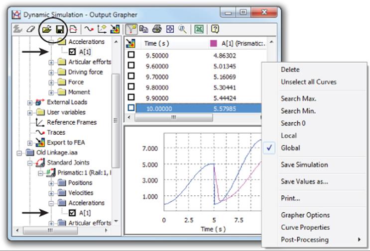
Figure 17.37 An imported acceleration curve

Also shown in Figure 17.37, the context menu is obtained by right-clicking either of the curve columns. From this menu you can search for the minimum and maximum values as well as zero values. You can also select Curve Properties and change the curve colors as well as analyze the average, minimum, maximum, median, standard deviation, and amplitude of the curve.

Exporting to FEA

You can use the Output Grapher to identify maximum forces and then export those forces for use in the Stress Analysis environment. Although the maximum stress is likely the most common value to be exported, you can export the force for any time step in the simulation. This can be useful when trying to focus on a particular event in the simulation. Here are the steps for exporting a maximum force:

1. Select that force in the left pane of the Output Grapher.

2. Right-click and choose Search Max.

3. Select the check box for the time step identified as the maximum value.

4. Click the Export To FEA button in the Output Grapher or on the Dynamic Simulation tab.

5. Select the part or parts to export the load information to.

6. Select the load-bearing faces on the part or parts.

Figure 17.38 shows the steps involved in exporting the time step to FEA. Notice that once the time step is exported, it is listed in the Export To FEA node in the Output Grapher browser. You should also note that you can export multiple time steps at once by selecting them all before clicking the Export To FEA button.

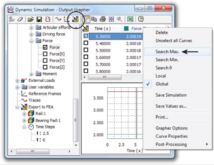
Figure 17.38 Exporting a maximum load time step to FEA

Using the Dynamic Simulation Information in Stress Analysis

Once you've exported the information from the Dynamic Simulation environment, you can select the Environments tab and click the Stress Analysis button to enter that environment. Follow these steps:

1. Click the Create Simulation button, or right-click an existing simulation and choose Edit Simulation Properties.

2. In the Simulation Properties dialog box, select the Motion Loads Analysis check box and then select the part and time step on which you intend to run the simulation analysis. Then click the OK button.

3. Make modifications to the simulation parameters if needed and then run the simulation.

You should note that a motion-loads analysis is limited to a single part occurrence and a single time step, per simulation. You can create multiple simulations to consider other time stamps or parts. All other components are automatically excluded from the simulation for motion loads. Figure 17.39 shows the Motion Loads Analysis option in the Simulation Properties dialog box.

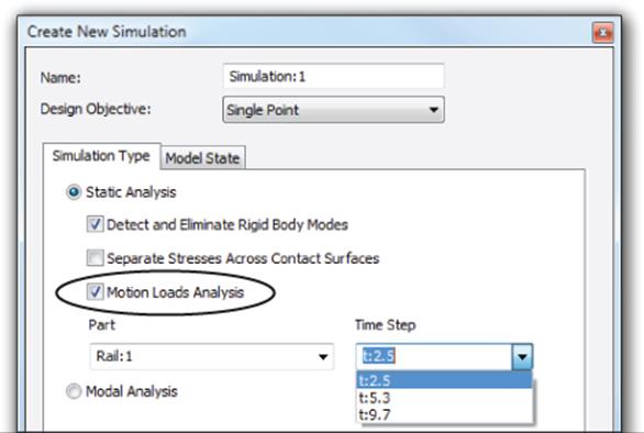
Figure 17.39 Enabling motion loads from dynamic simulation

The Bottom Line

1. Set up and run Stress Analysis simulations. Oftentimes you may find yourself guessing at what impact a change to your design might have on the strength and overall integrity of your part. Questions such as “Can I make this part a bit lighter?” or “Can I move this cutout closer to the edge?” become important to the success of your design.

1. Master It Set up a parameter study in your model to explore the consequences of editing features and their locations. Nominate all the crucial parameters to the table and then create the configuration simulations for all of the combinations.

2. Set up and run Dynamic Simulations. When you find yourself working out the details of a design with many moving parts, consider using the Dynamic Simulation tools early in the process to prove what will or will not work before going forward.

1. Master It Even before the assembly is complete, switch to the Dynamic Simulation environment and create assembly relationships in the simulation. Test the motion as you build the parts, and attempt to understand how contact will occur from the beginning.

3. Export results from the Dynamic Simulation environment to the Stress Analysis environment. Often when setting up a stress analysis simulation, you are guessing at what the loads might be, based on rough calculations. As you make changes to the design, those calculations become out-of-date and therefore invalid.

1. Master It How do you use the Dynamic Simulation tools to determine the force exerted on one part by another?