Essential MATLAB for Engineers and Scientists (2013)
PART 1
Essentials
OUTLINE
Introduction
Chapter 1. Introduction
Chapter 2. MATLAB Fundamentals
Chapter 3. Program Design and Algorithm Development
Chapter 4. MATLAB Functions and Data Import-Export Utilities
Chapter 5. Logical Vectors
Chapter 6. Matrices and Arrays
Chapter 7. Function M-files
Chapter 8. Loops
Chapter 9. MATLAB Graphics
Chapter 10. Vectors as Arrays and Other Data Structures
Chapter 11. Errors and Pitfalls
Introduction
Part 1 concerns those aspects of MATLAB that you need to know in order to come to grips with MATLAB's essentials and those of technical computing. Because this book is a tutorial, you are encouraged to use MATLAB extensively while you go through the text.
CHAPTER 1
Introduction
Abstract
The objectives of this chapter are to enable you to use some simple MATLAB commands from the Command Window, to examine various MATLAB desktop and editing features, to learn some of the new features of the MATLAB R2016a Desktop, to learn to write scripts in the Editor and Run them from the Editor, and to learn some of the new features associated with the tabs (in particular, the PUBLISH and APPS features). In this chapter you learn that MATLAB is a matrix-based computer system designed to assist in scientific and engineering problem solving. You also learn that one way to use MATLAB is to enter commands and statements on the command line in the Command Window. In this case the commands you enter are carried out immediately. You are also introduced to a number of useful built-in commands and functions.
Keywords
MATLAB R2016a; Elementary commands; Editing and executing commands
CHAPTER OUTLINE
Using MATLAB
Arithmetic
Variables
Mathematical functions
Functions and commands
Vectors
Linear equations
Tutorials and demos
The desktop
Using the Editor and running a script
Help, publish and view
Symbolics and the MuPAD notebook APP
Other APPS
Additional features
Sample program
Cut and paste
Saving a program: script files
Current directory
Running a script from the current folder browser
A program in action
Summary
Exercises
Supplementary material
THE OBJECTIVES OF THIS CHAPTER ARE:
■ To enable you to use some simple MATLAB commands from the Command Window.
■ To examine various MATLAB desktop and editing features.
■ To learn some of the new features of the MATLAB R2016a Desktop.
■ To learn to write scripts in the Editor and Run them from the Editor.
■ To learn some of the new features associated with the tabs (in particular, the PUBLISH and APPS features).
MATLAB is a powerful technical computing system for handling scientific and engineering calculations. The name MATLAB stands for Matrix Laboratory, because the system was designed to make matrix computations particularly easy. A matrix is an array of numbers organized in m rows and n columns. An example is the following ![]() array:
array:
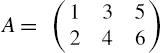
Any one of the elements in a matrix can be plucked out by using the row and column indices that identify its location. The elements in this example are plucked out as follows: ![]() ,
, ![]() ,
, ![]() ,
, ![]() ,
, ![]() ,
, ![]() . The first index identifies the row number counted from top to bottom; the second index is the column number counted from left to right. This is the convention used in MATLAB to locate information in an array. A computer is useful because it can do numerous computations quickly, so operating on large numerical data sets listed in tables as arrays or matrices of rows and columns is quite efficient.
. The first index identifies the row number counted from top to bottom; the second index is the column number counted from left to right. This is the convention used in MATLAB to locate information in an array. A computer is useful because it can do numerous computations quickly, so operating on large numerical data sets listed in tables as arrays or matrices of rows and columns is quite efficient.
This book assumes that you have never used a computer before to do the sort of scientific calculations that MATLAB handles, but are able to find your way around a computer keyboard and know your operating system (e.g., Windows, UNIX or MAC-OS). The only other computer-related skill you will need is some very basic text editing.
One of the many things you will like about MATLAB (and that distinguishes it from many other computer programming systems, such as C++ and Java) is that you can use it interactively. This means you type some commands at the special MATLAB prompt and get results immediately. The problems solved in this way can be very simple, like finding a square root, or very complicated, like finding the solution to a system of differential equations. For many technical problems, you enter only one or two commands—MATLAB does most of the work for you.
There are three essential requirements for successful MATLAB applications:
■ You must learn the exact rules for writing MATLAB statements and using MATLAB utilities.
■ You must know the mathematics associated with the problem you want to solve.
■ You must develop a logical plan of attack—the algorithm—for solving a particular problem.
This chapter is devoted mainly to the first requirement: learning some basic MATLAB rules. Computer programming is a precise science (some would also say an art); you have to enter statements in precisely the right way. There is a saying among computer programmers: Garbage in, garbage out. It means that if you give MATLAB a garbage instruction, you will get a garbage result.
With experience, you will be able to design, develop and implement computational and graphical tools to do relatively complex science and engineering problems. You will be able to adjust the look of MATLAB, modify the way you interact with it, and develop a toolbox of your own that helps you solve problems of interest. In other words, you can, with significant experience, customize your MATLAB working environment.
As you learn the basics of MATLAB and, for that matter, any other computer tool, remember that applications do nothing randomly. Therefore, as you use MATLAB, observe and study all responses from the command-line operations that you implement, to learn what this tool does and does not do. To begin an investigation into the capabilities of MATLAB, we will do relatively simple problems that we know the answers because we are evaluating the tool and its capabilities. This is always the first step. As you learn about MATLAB, you are also going to learn about programming, (1) to create your own computational tools, and (2) to appreciate the difficulties involved in the design of efficient, robust and accurate computational and graphical tools (i.e., computer programs).
In the rest of this chapter we will look at some simple examples. Don't be concerned about understanding exactly what is happening. Understanding will come with the work you need to do in later chapters. It is very important for you to practice with MATLAB to learn how it works. Once you have grasped the basic rules in this chapter, you will be prepared to master many of those presented in the next chapter and in the Help files provided with MATLAB. This will help you go on to solve more interesting and substantial problems. In the last section of this chapter you will take a quick tour of the MATLAB desktop.
1.1. Using MATLAB
Either MATLAB must be installed on your computer or you must have access to a network where it is available. Throughout this book the latest version at the time of writing is assumed (Version R2016a).
To start from Windows, double-click the MATLAB icon on your Windows desktop. To start from UNIX, type matlab at the operating system prompt. To start from MAC-OS open X11 (i.e., open an X-terminal window), then type matlab at the prompt. The MATLAB desktop opens as shown in Figure 1.1. The window in the desktop that concerns us for now is the Command Window, where the special >> prompt appears. This prompt means that MATLAB is waiting for a command. You can quit at any time with one of the following ways:
■ Click the X (close box) in the upper right-hand corner of the MATLAB desktop.
■ Type quit or exit at the Command Window prompt followed by pressing the ‘enter’ key.
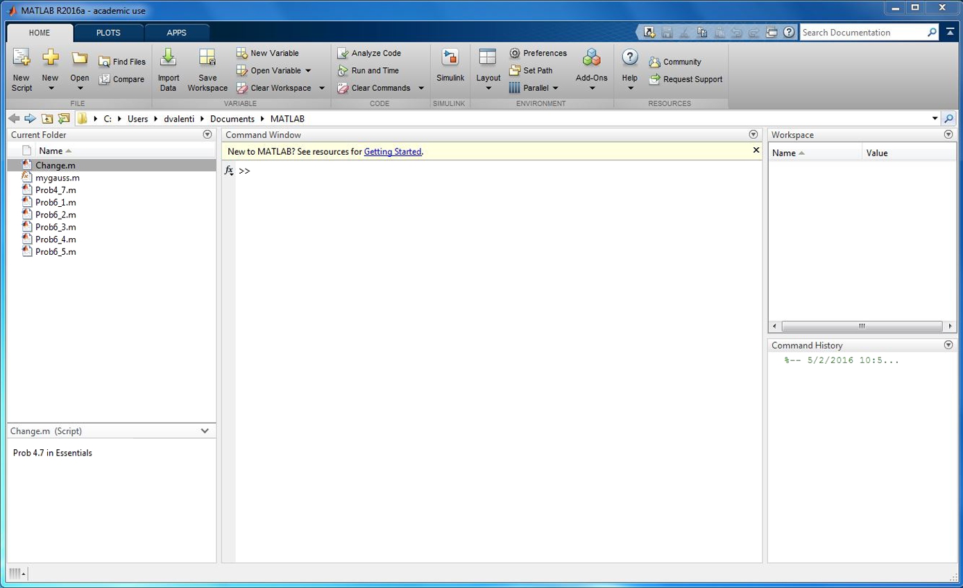
FIGURE 1.1 MATLAB desktop illustrating the Home task bar (version 2016a).
Starting MATLAB automatically creates a folder named MATLAB in the user's Documents Folder. This feature is quite convenient because it is the default working folder. It is in this folder that anything saved from the Command Window will be saved. Now you can experiment with MATLAB in the Command Window. If necessary, make the Command Window active by placing the cursor in the Command Window and left-clicking the mouse button anywhere inside its border.
1.1.1. Arithmetic
Since we have experience doing arithmetic, we want to examine if MATLAB does it correctly. This is a required step to gain confidence in any tool and in our ability to use it.
Type 2+3 after the >> prompt, followed by Enter (press the Enter key) as indicated by <Enter>:
>> 2+3 <Enter>
Commands are only carried out when you enter them. The answer in this case is, of course, 5. Next try
>> 3-2 <Enter>
>> 2*3 <Enter>
>> 1/2 <Enter>
>> 23 <Enter>
>> 2\11 <Enter>
What about (1)/(2) and (2)^(3)? Can you figure out what the symbols *, /, and ^ mean? Yes, they are multiplication, division and exponentiation. The backslash means the denominator is to the left of the symbol and the numerator is to the right; the result for the last command is 5.5. This operation is equivalent to 11/2.
Now enter the following commands:
>> 2 .* 3 <Enter>
>> 1 ./ 2 <Enter>
>> 2 .̂ 3 <Enter>
A period in front of the *, /, and ^, respectively, does not change the results because the multiplication, division, and exponentiation is done with single numbers. (An explanation for the need for these symbols is provided later when we deal with arrays of numbers.)
Here are hints on creating and editing command lines:
■ The line with the >> prompt is called the command line.
■ You can edit a MATLAB command before pressing Enter by using various combinations of the Backspace, Left-arrow, Right-arrow, and Del keys. This helpful feature is called command-line editing.
■ You can select (and edit) commands you have entered using Up-arrow and Down-arrow. Remember to press Enter to have the command carried out (i.e., to run or to execute the command).
■ MATLAB has a useful editing feature called smart recall. Just type the first few characters of the command you want to recall. For example, type the characters 2* and press the Up-arrow key—this recalls the most recent command starting with 2*.
How do you think MATLAB would handle 0/1 and 1/0? Try it. If you insist on using ∞ in a calculation, which you may legitimately wish to do, type the symbol Inf (short for infinity). Try 13+Inf and 29/Inf.
Another special value that you may meet is NaN, which stands for Not-a-Number. It is the answer to calculations like 0/0.
1.1.2. Variables
Now we will assign values to variables to do arithmetic operations with the variables. First enter the command (statement in programming jargon) a = 2. The MATLAB command line should look like this:
>> a = 2 <Enter>
The a is a variable. This statement assigns the value of 2 to it. (Note that this value is displayed immediately after the statement is executed.) Now try entering the statement a = a + 7 followed on a new line by a = a * 10. Do you agree with the final value of a? Do we agree that it is 90?
Now enter the statement
>> b = 3; <Enter>
The semicolon (;) prevents the value of b from being displayed. However, b still has the value 3, as you can see by entering without a semicolon:
>> b <Enter>
Assign any values you like to two variables x and y. Now see if you can assign the sum of x and y to a third variable z in a single statement. One way of doing this is
>> x = 2; y = 3; <Enter>
>> z = x + y <Enter>
Notice that, in addition to doing the arithmetic with variables with assigned values, several commands separated by semicolons (or commas) can be put on one line.
1.1.3. Mathematical functions
MATLAB has all of the usual mathematical functions found on a scientific-electronic calculator, like sin, cos, and log (meaning the natural logarithm). See Appendix B.5 for many more examples.
■ Find ![]() with the command sqrt(pi). The answer should be 1.7725. Note that MATLAB knows the value of pi because it is one of its many built-in functions.
with the command sqrt(pi). The answer should be 1.7725. Note that MATLAB knows the value of pi because it is one of its many built-in functions.
■ Trigonometric functions like sin(x) expect the argument x to be in radians. Multiply degrees by ![]() to get radians. For example, use MATLAB to calculate
to get radians. For example, use MATLAB to calculate ![]() . The answer should be 1 (sin(90*pi/180)).
. The answer should be 1 (sin(90*pi/180)).
■ The exponential function ![]() is computed in MATLAB as exp(x). Use this information to find e and
is computed in MATLAB as exp(x). Use this information to find e and ![]() (2.7183 and 0.3679).
(2.7183 and 0.3679).
Because of the numerous built-in functions like pi or sin, care must be taken in the naming of user-defined variables. Names should not duplicate those of built-in functions without good reason. This problem can be illustrated as follows:
>> pi = 4 <Enter>
>> sqrt(pi) <Enter>
>> whos <Enter>
>> clear pi <Enter>
>> whos <Enter>
>> sqrt(pi) <Enter>
>> clear <Enter>
>> whos <Enter>
Note that clear executed by itself clears all local variables in the workspace; >>clear pi clears the locally defined variable pi. In other words, if you decide to redefine a built-in function or command, the new value is used! The command whos is executed to determine the list of local variables or commands presently in the workspace. The first execution of the command pi = 4 in the above example displays your redefinition of the built-in pi: a 1-by-1 (or 1x1) double array, which means this data type was created when pi was assigned a number (you will learn more about other data types later, as we proceed in our investigation of MATLAB).
1.1.4. Functions and commands
MATLAB has numerous general functions. Try date and calendar for starters. It also has numerous commands, such as clc (for clear command window). help is one you will use a lot (see below). The difference between functions and commands is that functions usually return with a value (e.g., the date), while commands tend to change the environment in some way (e.g., clearing the screen or saving some statements to the workspace).
1.1.5. Vectors
Variables such as a and b that were used in Section 1.1.2 above are called scalars; they are single-valued. MATLAB also handles vectors (generally referred to as arrays), which are the key to many of its powerful features. The easiest way of defining a vector where the elements (components) increase by the same amount is with a statement like
>> x = 0 : 10; <Enter>
That is a colon (:) between the 0 and the 10. There is no need to leave a space on either side of it, except to make it more readable. Enter x to check that x is a vector; it is a row vector—consisting of 1 row and 11 columns. Type the following command to verify that this is the case:
>> size(x) <Enter>
Part of the real power of MATLAB is illustrated by the fact that other vectors can now be defined (or created) in terms of the just defined vector x. Try
>> y = 2 .* x <Enter>
>> w = y ./ x <Enter>
and
>> y = sin(x) <Enter>
(no semicolons). Note that the first command line creates a vector y by multiplying each element of x by the factor 2. The second command line is an array operation, creating a vector w by taking each element of y and dividing it by the corresponding element of x. Since each element of y is two times the corresponding element of x, the vector w is a row vector of 11 elements all equal to 2. Finally, z is a vector with sin(x) as its elements.
To draw a reasonably nice graph of ![]() , simply enter the following commands:
, simply enter the following commands:
>> x = 0 : 0.1 : 10; <Enter>
>> z = sin(x); <Enter>
>> plot(x,z), grid <Enter>
The graph appears in a separate figure window. To draw the graph of the sine function illustrated in Figure 1.2 replace the last line above with
>> plot(x,y,'-rs','LineWidth',2,'MarkerEdgeColor','k','MarkerSize',5),grid
<Enter>
>> xlabel(' x '), ylabel(' sin(x) ') <Enter>
>> whitebg('y') <Enter>
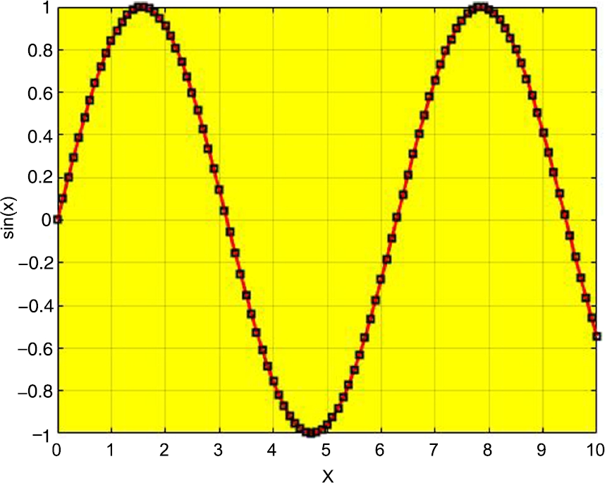
FIGURE 1.2 Figure window.
You can select the Command Window or figure windows by clicking anywhere inside them. The Windows pull-down menus can be used in any of them.
Note that the first command line above has three numbers after the equal sign. When three numbers are separated by two colons in this way, the middle number is the increment. The increment of 0.1 was selected to give a reasonably smooth graph. The command grid following the comma in the last command line adds a grid to the graph.
Modifying the plot function as illustrated above, of the many options available within this function, four were selected. A comma was added after the variable y followed by '-rs'. This selects a solid red line (-r) to connect the points at which the sine is computed; they are surrounded by square (s) markers in the figure. The line width is increased to 2 and the marker edge color is black (k) with size 5. Axis labels and the background color were changed with the statements following the plot command. (Additional changes in background color, object colors etc. can be made with the figure properties editor; it can be found in the pull-down menu under Edit in the figure toolbar. Many of the colors in the figures in this book were modified with the figure-editing tools.)
If you want to see more cycles of the sine graph, use command-line editing to change sin(x) to sin(2*x).
Try drawing the graph of tan(x) over the same domain. You may find aspects of your graph surprising. To help examine this function you can improve the graph by using the command axis([0 10 -10 10]) as follows:
>> x = 1:0.1:10; <Enter>
>> z = tan(x); <Enter>
>> plot(x,z),axis([0 10 -10 10]) <Enter>
An alternative way to examine mathematical functions graphically is to use the following command:
>> ezplot('tan(x)') <Enter>
The apostrophes around the function tan(x) are important in the ezplot command. Note that the default domain of x in ezplot is not 0 to 10.
A useful Command Window editing feature is tab completion: Type the first few letters of a MATLAB name and then press Tab. If the name is unique, it is automatically completed. If it is not unique, press Tab a second time to see all the possibilities. Try by typing ta at the command line followed by Tab twice.
1.1.6. Linear equations
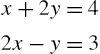
Systems of linear equations are very important in engineering and scientific analysis. A simple example is finding the solution to two simultaneous equations:
Here are two approaches to the solution.
Matrix method. Type the following commands (exactly as they are):
>> a = [1 2; 2 -1]; <Enter >
>> b = [4; 3]; <Enter >
>> x = a\b <Enter >
The result is
x =
2
1
i.e., ![]() ,
, ![]() .
.
Built-in solve function. Type the following commands (exactly as they are):
>> [x,y] = solve('x+2*y=4','2*x - y=3') <Enter >
>> whos <Enter >
>> x = double(x), y=double(y) <Enter >
>> whos <Enter >
The function double converts x and y from symbolic objects (another data type in MATLAB) to double arrays (i.e., the numerical-variable data type associated with an assigned number).
To check your results, after executing either approach, type the following commands (exactly as they are):
>> x + 2*y % should give ans = 4 <Enter >
>> 2*x - y % should give ans = 3 <Enter >
The % symbol is a flag that indicates all information to the right is not part of the command but a comment. (We will examine the need for comments when we learn to develop coded programs of command lines later on.)
1.1.7. Tutorials and demos
If you want a spectacular sample of what MATLAB has to offer, type the command demo on the command line. After entering this command the Help documentation is opened at MATLAB Examples (see Figure 1.3). Left-click on “Getting Started”. This points you to the list of tutorials and demonstrations of MATLAB applications that are at your disposal. Click on any of the other topics to learn more about the wealth of capabilities of MATLAB. You may wish to review the tutorials appropriate to the topics you are examining as part of your technical computing needs. Scroll down to the “New Features Video” to learn more about the Desktop and other new features, some of which are introduced next.
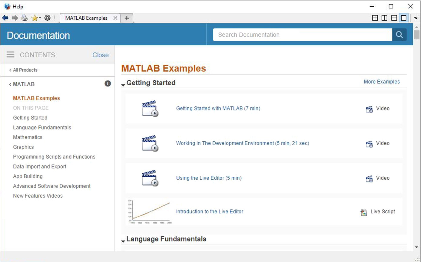
FIGURE 1.3 The Help documentation on MATLAB Examples.
1.2. The desktop
A very useful feature of MATLAB R2016a is the fact that when you first open it, it creates the folder named MATLAB (if it does not already exist) in your Documents folder. The first time it does this, there are no items in the folder and, hence, the Current Folder panel will be empty. This new folder in your Documents is the default working folder where all the files your create are saved. The location of this folder is given in the first toolbar above the Command Window. The location is C:\Users\Clara\Documents\MATLAB. This format of the location was determined by pointing and left-clicking the mouse in the line just above the Command Window.
Let us examine the Desktop from the top down. On the left side of the top line you should see the name of the version of MATLAB running. In this case it is MATLAB R2016a. On the right side of the top line are three buttons. They are the underscore button, which allows you to minimize the size of the Desktop window, the rectangle button, which allows you to maximize the size of the Desktop, and the × button, which allows you to close MATLAB (see Figure 1.4).
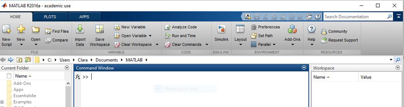
FIGURE 1.4 New Desktop Toolbar on MATLAB 2016a.
On the next line of the Desktop there are three tabs on the left side. The first tap is most forward in the figure and, hence, the Home toolbar is displayed (the tabs and the toolbars associated with the tabs are the main new features of this release of MATLAB). If you are already familiar with a previous release of MATLAB, you will find that these new features enhance significantly the use of MATLAB. In addition, all previously developed tools operate exactly as they did in previous releases of MATLAB. The other two tabs are PLOTS and APPS. These features allow you to access tools within MATLAB by pointing and clicking and, hence, enhance the utilization of tools and toolboxes available within MATLAB. In addition, the APPS environment allows the user to create their own applications (or APPS).
1.2.1. Using the Editor and running a script
Point and click on the New Script icon on the left most side of the Home toolbar. Doing this opens the editor in the center of the Desktop as shown in Figure 1.5. Note that three new tabs appear and that the tab that is visible is the Editor tab that is connected with the Editor. The other two tabs are Publish and View. The latter are useful when creating notebooks or other documents connected with your technical computing work. The application of these tools will be illustrated by an example later in this text.
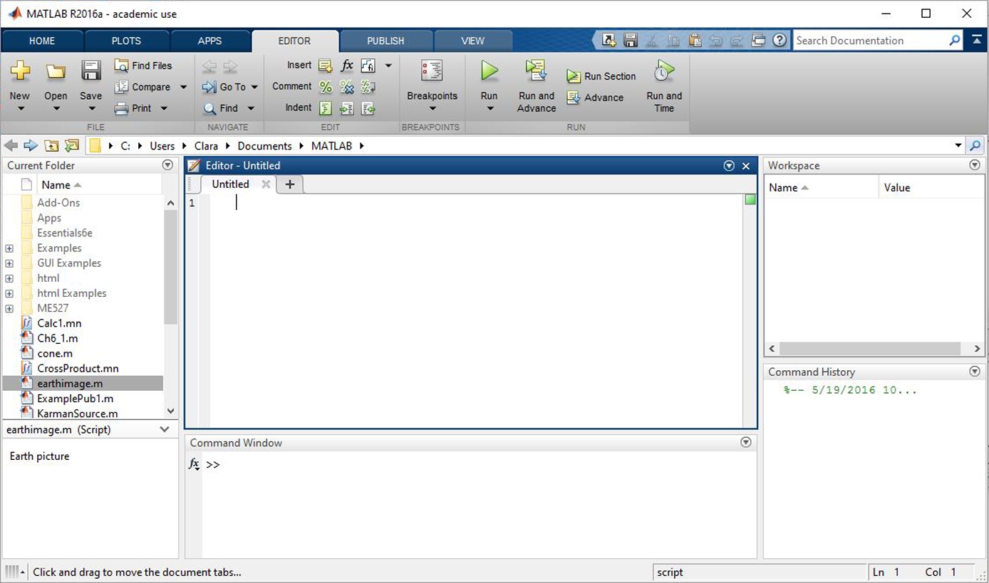
FIGURE 1.5 Editor opened in default location; it is in the center of the Desktop.
Let us first consider using the Editor. Type into the Editor the following script:
% Example of one of the matrix inversion methods available in MATLAB
clear;clc
% Let us consider the following arbitrarily selected matrix:
A =magic(3)
% Let us evaluate its inverse as follows:
AI = inv(A)
% Let us check that it is an inverse:
IPredicted = A * AI
% This is the exact unitary matrix:
IM = eye(3)
% The is the difference between the exact and predict unitary
% matrix:
difference = IPredicted - IM
for m = 1:3
for n = 1:3
if difference(m,n) < eps;
IPredicted(m,n) = IM(m,n);
end
end
end
IPredicted
IPredicted == IM
Then click on the Run button just under the tab named View. The first time the script is executed you are asked to name the file. The name used in this example is ExA1_1.m. If all lines are typed correctly (except the lines beginning with the symbol '%', because they are comments that have nothing to do with the sequence of commands in the script except that they help the reader understand what the script does), what shows up in the Command Window is as follows:
A =
8 1 6
3 5 7
4 9 2
AI =
0.1472 -0.1444 0.0639
-0.0611 0.0222 0.1056
-0.0194 0.1889 -0.1028
IPredicted =
1.0000 0 -0.0000
-0.0000 1.0000 0
0.0000 0 1.0000
IM =
1 0 0
0 1 0
0 0 1
difference =
1.0e-15 *
0 0 -0.1110
-0.0278 0 0
0.0694 0 0
IPredicted =
1 0 0
0 1 0
0 0 1
ans =
1 1 1
1 1 1
1 1 1
The IPredicted matrix is supposed to be the identity matrix, IM. The matrix IPredicted was determined by multiplying the matrix A by its numerically computed inverse, AI. The last print out of IPredicted is a modification of the original matrix; it was changed to the elements of the IM matrix if the difference between a predicted and an actual element of IM was less than eps ![]() . Since the result is identical to the identity matrix, this shows that the inverse was computed correctly (at least to within the computational error of the computing environment, i.e., 0< eps). This conclusion is a result of the fact that the ans in the above example produced the logical result of 1 (or true) for all entries in the adjusted IPredicted matrix as logically compared with the corresponding entries in IM.
. Since the result is identical to the identity matrix, this shows that the inverse was computed correctly (at least to within the computational error of the computing environment, i.e., 0< eps). This conclusion is a result of the fact that the ans in the above example produced the logical result of 1 (or true) for all entries in the adjusted IPredicted matrix as logically compared with the corresponding entries in IM.
At this point in the exercise the Desktop looks like Figure 1.6. The name of the file is ExA1_1.m. It appears in the Current Folder and it also appears in the Command History. Note that the Workspace is populated with the variables created by this script.
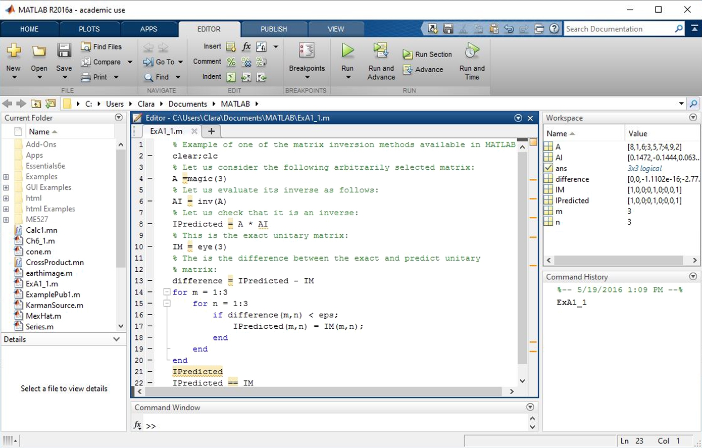
FIGURE 1.6 Sample script created and executed in the first example of this section.
This concludes the introduction of the most important tools needed for most of the exercises in Essential MATLAB (i.e., in this text). In the next section we examine an example of some of the other new features of MATLAB R2016a.
1.2.2. Help, publish and view
Publish is an easy way to create notebooks or other documents in html format. The conversion of the information typed into an M-file is published into a document that looks like the new Help environment. To open the help documents go to the top of the Desktop to the question mark. Left click on the question mark ?. The Help window opens up. Left click on the topic “MATLAB” to open up the window illustrated in Figure 1.7. This also illustrates the new format of the searchable documentation available within MATLAB R2016a. We want to compare this documentation with the kind you can PUBLISH yourself. To illustrate how easy it is to create documents like the MATLAB documents, let us consider the following simple example.
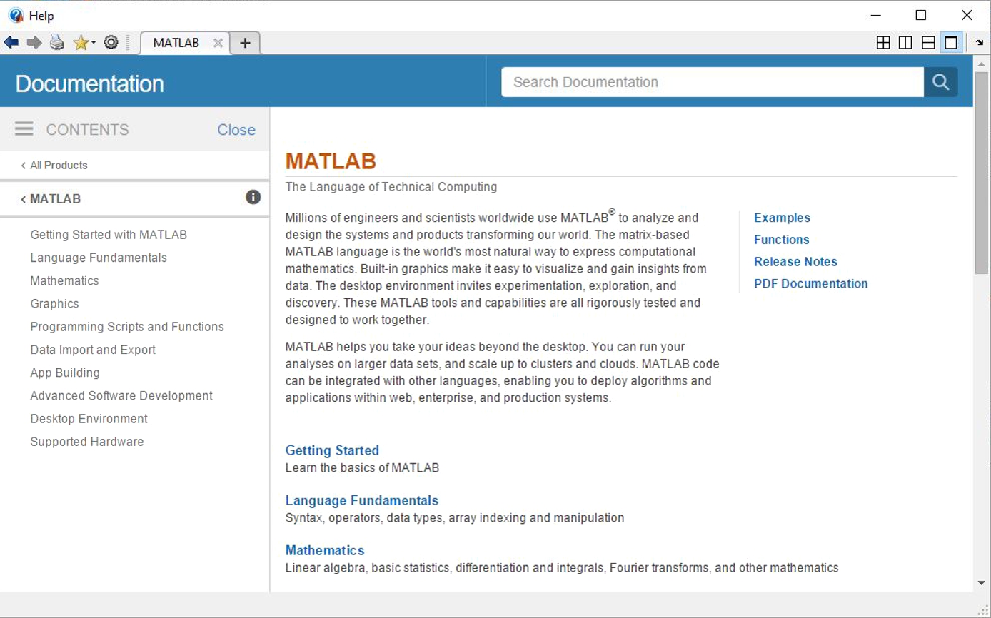
FIGURE 1.7 Illustration of one of the pages in the online documentation for MATLAB.
Click the New Script button to open up the editor (or type edit after the command prompt in the Command Window followed by tapping the enter key). The Editor tab is in the most forward position on the main taskbar. Place the cursor on PUBLISH and left click on the mouse. This brings the PUBLISH toolbar forward. Left click Section with Title. Replace SECTION TITLE with PUBLISHING example. Next, replace DESCRIPTIVE TEXT with
%%
% This is an example to illustrate how easy it is to create a document
% in the PUBLISH environment.
%
% (1) This is an illustration of a formula created with a LaTeX command:
%
Next, click on Σ Inline LaTeX located in the “Insert Inline Markup” group. This leads to the addition of the equation $x^2+e^{\pi i}$. Following this equation add the text shown in the final script file shown below that ends with “clicked:”. This is followed by a blank line and a command script; this command script is included to illustrate how MATLAB commands can be incorporated into published documents.
%%
% This is an example to illustrate how easy it is to create a document
% in the PUBLISH environment.
%
% (1) This is an illustration of a formula created with a LaTeX command:
%
%%
% $x^2+e^{\pi i}$
%
% (2) This is an illustration of how you can incorporate a MATLAB script
% in the document that is run when the Publish button below and to the
% right of View is clicked:
% Earth picture
load earth
image(X); colormap(map);
axis image
The final step is to left-click on Publish, which is just to the right and below View. The first window to appear is the one asking you to save the M-file. The name used in this example is ExamplePub1.m. After it appears in the Current Folder it is executed. A folder named html is automatically created and it contains the html document just created. The document is illustrated in Figure 1.8.
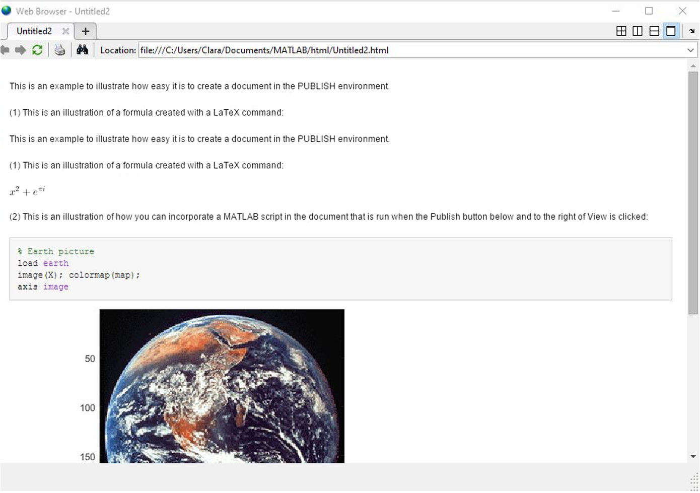
FIGURE 1.8 Sample document created in the Publish environment.
Finally, the VIEW tab brings up a toolbar that allows you to change the configuration of the Editor window. From the authors point of view, the default Editor environment is fine as is especially for users who are beginning to use MATLAB for technical computing. Customizing your working environment is certainly possible in MATLAB. However, it is useful to learn how to deal with the default environment before deciding what needs to be changed to help satisfy your own requirements for using MATLAB.
1.2.3. Symbolics and the MuPAD notebook APP
The Symbolic Math Toolbox is a useful tool to help you do symbolic mathematical analysis. It has been made much more accessible through the application called the MuPAD Notebook APP. To open this APP start by a left-click on the APPS tab in the second line from the top on the desktop shown in Figure 1.4. This operation brings the APPS toolbar forward as illustrated in Figure 1.9. Left-click on the MuPAD Notebook APP. The window in Figure 1.10 is the notebook environment that opens up. The left bracket on the upper left side of the white note pad is where the commands are typed. The panel on the right side of the pad is the Command Bar. It provides easy access to many of the commands needed to do mathematics including the manipulation and evaluation of mathematical expressions as well as plotting graphs. The two toolbars above the pad provide useful utilities to enhance your usage of MuPAD. Moving the cursor over the items on the second line tells you what each button does. The first line requires moving the cursor over them and a left-click on the mouse to open the pull-down menu. This toolbar is common to all windows of the MATLAB technical computing environment. Let us examine a simple example.
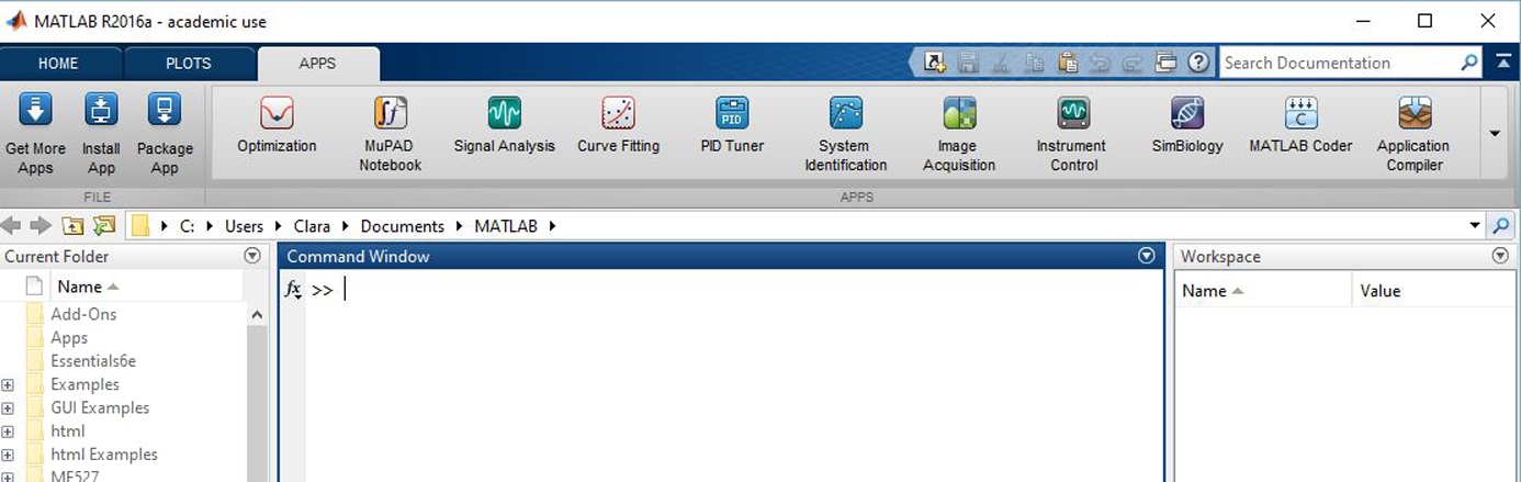
FIGURE 1.9 The APPS toolbar on the Desktop.
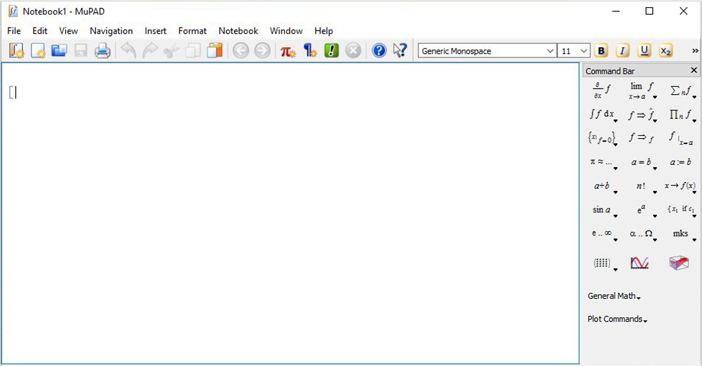
FIGURE 1.10 The MuPAD window or notebook.
Left-click in the note pad just above the left bracket. At this location you can start typing text (i.e., your notes on the mathematical work you are about to begin in this notebook). Figure 1.11 illustrates a simple example of taking the derivative of a function and then integrating the result to learn more about the relationship between differentiation and integration in the calculus. This notebook was saved under the name Calc1.mn. Note the file extension (‘*.mn’) for MATLAB notebooks created in MuPAD. Double-left clicking on the file with this filename in the Command Folder panel opens this notebook (as it is illustrated in the figure). The details of this example are also provided in the figure. They are as follows:
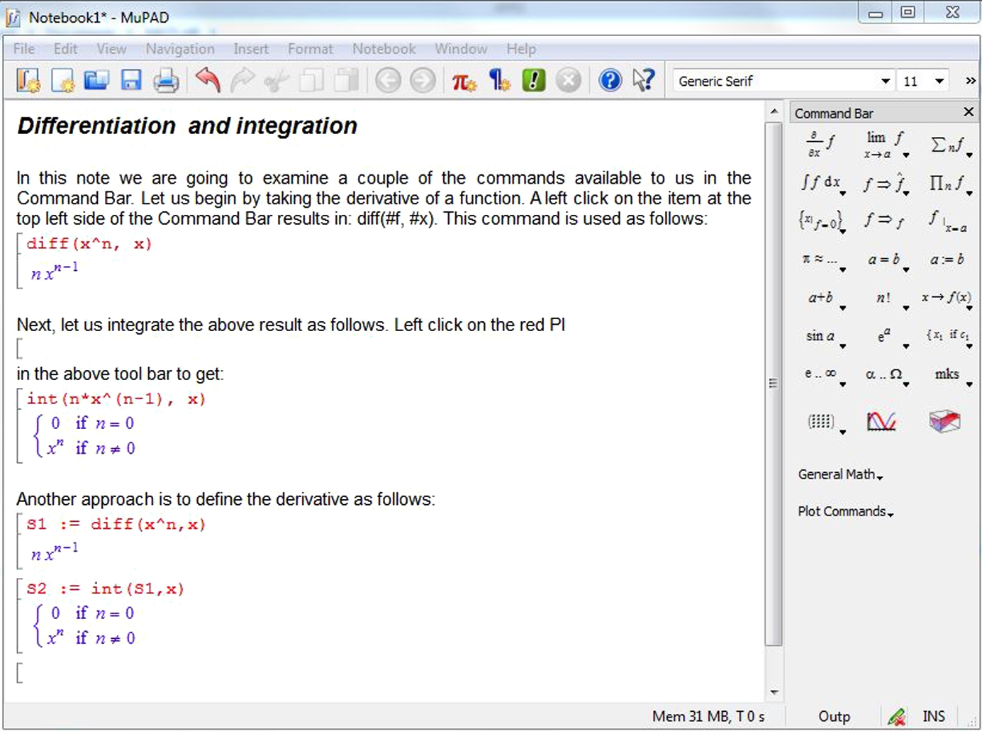
FIGURE 1.11 The MuPAD notebook Calc1.mn.
Differentiation and integration In this note we are going to examine a few of the mathematical commands available to us and listed in the Command Bar. Let us begin with taking the derivative of a function f. With the cursor placed on the upper left most symbol, a left-click on the mouse produces the following result: diff(#f, #x). The # sign is a place holder at which input is required. The next step is to point to the right of the left bracket below and left-click to place the note pad cursor at this location. Then click on the command of interest in the Command Bar. Change #f to ![]() and #x to x. Then hit enter to execute the command. The result is:
and #x to x. Then hit enter to execute the command. The result is:
[diff(x^n, x)
![]()
Next, let us integrate this result. First let us save the result under the name S1 as follows:
[S1 := diff(x^n, x)
![]()
Now, let us integrate. Left-click on this operation in the Command Bar to get: int(#f, #x). Replace #f with S1 and #x with x. Thus,
[S2 := int(S1,x)
![]()
Hence, integration is, as expected, the inverse of differentiation. The only issue, if any, that you must keep in mind is that the constants of integration are set to zero. If you need to explicitly carry them along in your analysis, then you must add a constant to the results at this step.
REMARK: Help is available through the help documentation. The help can be accessed by a left click on the blue circle with the question mark in the toolbar just above this pad.
A second example is the graphics capabilities in MuPAD. There are other plotting utilities within MATLAB that allow you to examine functions graphically and quickly. The MuPAD environment is particularly well suited for this kind of investigation. Suppose you are reading a technical article and you come across two interesting functions and you want to have an idea as to what they look like. Let us examine two examples. One is the ![]() function which plays an important role in nonlinear wave theory. The second is the complete elliptic integral of the first kind, viz.,
function which plays an important role in nonlinear wave theory. The second is the complete elliptic integral of the first kind, viz.,
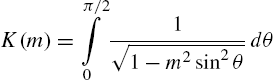
This integral plays an important role in potential theory. What do these functions look like? The MuPAD notebook in Figure 1.12 illustrates the shapes of these functions. More on these functions among other functions can be examined in the help documentation and in the references cited in the help documentation.
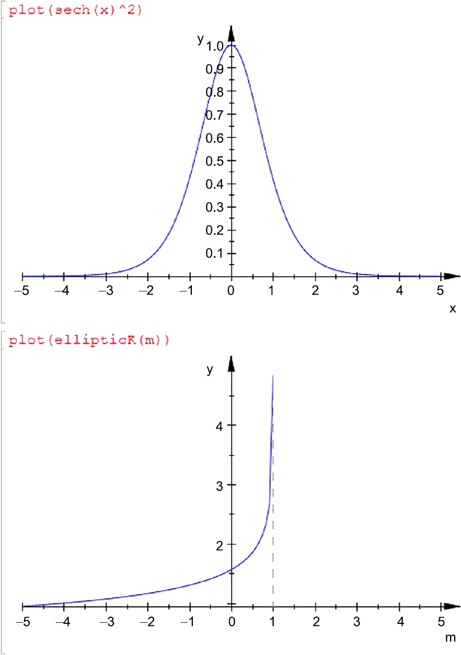
FIGURE 1.12 Illustration of MuPAD graphics.
This concludes this brief introduction to an APP and a brief introduction to the capabilities of the Symbolic Math toolbox.
1.2.4. Other APPS
There are a number of other APPS available from MathWorks. In addition, there is a capability for you to create your own APPS. Hence, if there is anything that we learn from our first experiences with MATLAB is that there is a lot to learn (a lifelong experience of learning) because of the wealth of technology incorporated in this technical computing environment. The fact that you can develop your own toolboxes, your own APPS and you can customize your working environment (desktop arrangement, color backgrounds, fonts, graphical user interfaces and so on) provides real opportunities and useful experience in creating designs, creating useful tools and documenting your work.
1.2.5. Additional features
MATLAB has other good things. For example, you can generate a 10-by-10 (or ![]() ) magic square by executing the command magic(10), where the rows, columns, and main diagonal add up to the same value. Try it. In general, an
) magic square by executing the command magic(10), where the rows, columns, and main diagonal add up to the same value. Try it. In general, an ![]() magic square has a row and column sum of
magic square has a row and column sum of ![]() .
.
You can even get a contour plot of the elements of a magic square. MATLAB pretends that the elements in the square are heights above sea level of points on a map, and draws the contour lines. contour(magic(32)) looks interesting.
If you want to see the famous Mexican hat (Figure 1.13), enter the following four lines (be careful not to make any typing errors):
>> [x y ] = meshgrid(-8 : 0.5 : 8); <Enter>
>> r = sqrt(x.^2 + y.^2) + eps; <Enter>
>> z = sin(r) ./ r; <Enter>
>> mesh(z); <Enter>
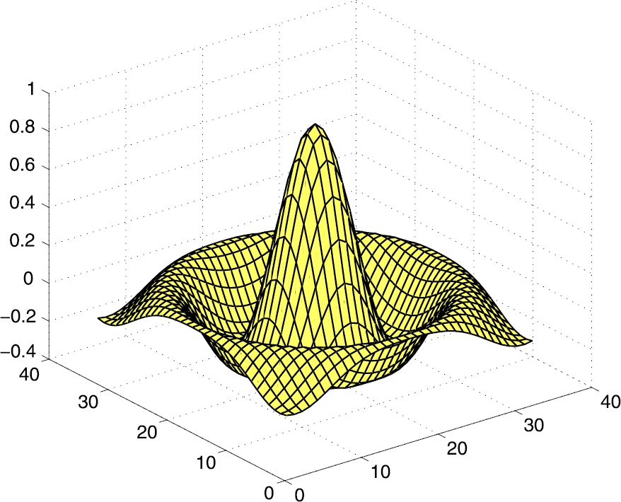
FIGURE 1.13 The Mexican hat.
surf(z) generates a faceted (tiled) view of the surface. surfc(z) or meshc(z) draws a 2D contour plot under the surface. The command
>> surf(z), shading flat <Enter>
produces a nice picture by removing the grid lines.
The following animation is an extension of the Mexican hat graphic in Figure 1.13. It uses a for loop that repeats the calculation from n = −3 to n = 3 in increments of 0.05. It begins with a for n = −3:0.05:3 command and ends with an end command and is one of the most important constructs in programming. The execution of the commands between the for and end statements repeat 121 times in this example. The pause(0.05) puts a time delay of 0.05 seconds in the for loop to slow the animation down, so the picture changes every 0.05 seconds until the end of the computation.
>> [x y]=meshgrid(-8:0.5:8); <Enter>
>> r=sqrt( x.^2+y.^2)+eps; <Enter>
>> for n=-3:0.05:3; <Enter>
>> z=sin(r.*n)./r; <Enter>
>> surf(z), view(-37, 38), axis([0,40,0,40,-4,4]); <Enter>
>> pause(0.05) <Enter>
>> end <Enter>
You can examine sound with MATLAB in any number of ways. One way is to listen to the signal. If your PC has a speaker, try
>> load handel <Enter>
>> sound(y,Fs) <Enter>
for a snatch of Handel's Hallelujah Chorus. For different sounds try loading chirp, gong, laughter, splat, and train. You have to run sound(y,Fs) for each one.
If you want to see a view of the Earth from space, try
>> load earth <Enter>
>> image(X); colormap(map) <Enter>
>> axis image <Enter>
To enter the matrix presented at the beginning of this chapter into MATLAB, use the following command:
>> A = [1 3 5; 2 4 6] <Enter>
On the next line after the command prompt, type A(2,3) to pluck the number from the second row, third column.
There are a few humorous functions in MATLAB. Try why (why not?) Then try why(2) twice. To see the MATLAB code that does this, type the following command:
>> edit why <Enter>
Once you have looked at this file, close it via the pull-down menu by clicking File at the top of the Editor desktop window and then Close Editor; do not save the file, in case you accidently typed something and modified it.
The edit command will be used soon to illustrate the creation of an M-file like why.m (the name of the file executed by the command why). You will create an M-file after we go over some of the basic features of the MATLAB desktop. More details on creating programs in the MATLAB environment will be explained in Chapter 2.
1.3. Sample program
In Section 1.1 we saw some simple examples of how to use MATLAB by entering single commands or statements at the MATLAB prompt. However, you might want to solve problems which MATLAB can't do in one line, like finding the roots of a quadratic equation (and taking all the special cases into account). A collection of statements to solve such a problem is called a program. In this section we look at the mechanics of writing and running two short programs, without bothering too much about how they work—explanations will follow in the next chapter.
1.3.1. Cut and paste
Suppose you want to draw the graph of ![]() over the domain 0 to 6π, as shown in Figure 1.14. The Windows environment lends itself to nifty cut and paste editing, which you would do well to master. Proceed as follows.
over the domain 0 to 6π, as shown in Figure 1.14. The Windows environment lends itself to nifty cut and paste editing, which you would do well to master. Proceed as follows.
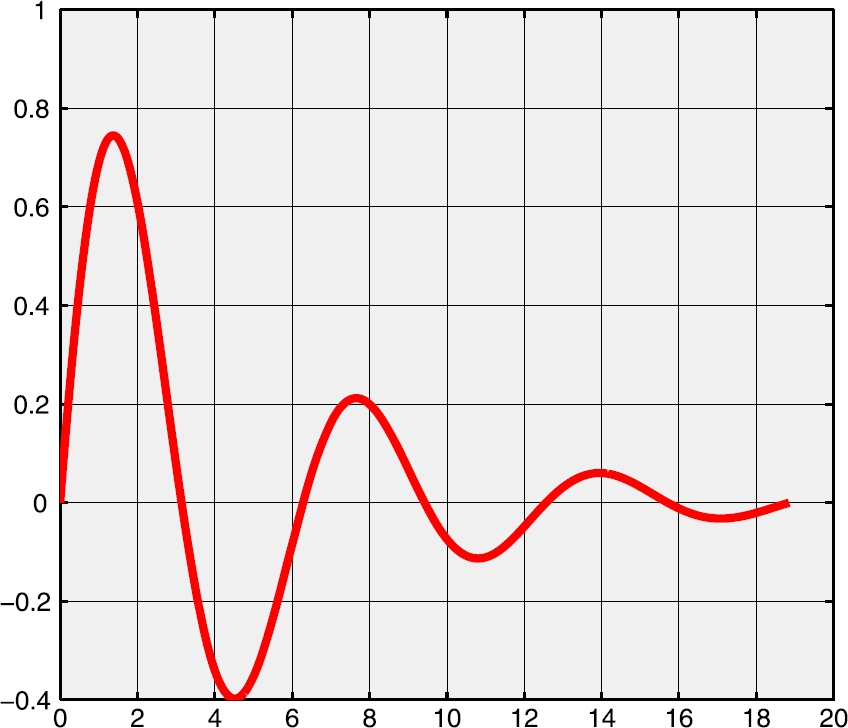
FIGURE 1.14 e![]() sin(x).
sin(x).
From the MATLAB desktop select File -> New -> Script, or click the new file button on the desktop toolbar (you could also type edit in the Command Window followed by Enter). This action opens an Untitled window in the Editor/Debugger. You can regard this for the time being as a ‘scratch pad’ in which to write programs. Now type the following two lines in the Editor, exactly as they appear here:
x = 0 : pi/20 : 6 * pi;
plot(x, exp(-0.2*x) .* sin(x), 'k'),grid
Incidentally, that is a dot (full stop, period) in front of the second * in the second line—a more detailed explanation later! The additional argument 'k' for plot will draw a black graph, just to be different. Change 'k' to 'r' to generate a red graph if you prefer.
Next, move the mouse pointer (which now looks like a very thin capital I) to the left of the x in the first line. Keep the left mouse button down while moving the mouse pointer to the end of the second line. This process is called dragging. Both lines should be highlighted at this stage, probably in blue, to indicate that they have been selected.
Select the Edit menu in the Editor window, and click on Copy (or just use the keyboard shortcut Ctrl+C). This action copies the highlighted text to the Windows clipboard, assuming that your operating system is Windows.
Now go back to the Command Window. Make sure the cursor is positioned at the >> prompt (click there if necessary). Select the Edit menu, and click on Paste (or use the Ctrl+V shortcut). The contents of the clipboard will be copied into the Command Window. To execute the two lines in the program, press Enter. The graph should appear in a figure window.
This process, from highlighting (selecting) text in the Editor, to copying it into the Command Window, is called ‘cut and paste’ (more correctly ‘copy and paste’ here, since the original text is copied from the Editor, rather than being cut from it). It's well worth practicing until you have it right.
If you need to correct the program, go back to the Editor, click at the position of the error (this moves the insertion point to the right place), make the correction, and cut and paste again. Alternatively, you can use command-line editing to correct mistakes. As yet another alternative, you can paste from the Command History window (which incidentally goes back over many previous sessions). To select multiple lines in the Command History window keep Ctrl down while you click.
If you prefer, you can enter multiple lines directly in the Command Window. To prevent the whole group from running until you have entered the last line use Shift+Enter after each line until the last. Then press Enter to run all the lines.
As another example, suppose you have $1000 saved in the bank. Interest is compounded at the rate of 9% per year. What will your bank balance be after one year? Now, if you want to write a MATLAB program to find your new balance, you must be able to do the problem yourself in principle. Even with a relatively simple problem like this, it often helps first to write down a rough structure plan:
1. Get the data (initial balance and interest rate) into MATLAB.
2. Calculate the interest (9% of $1000, i.e., $90).
3. Add the interest to the balance ($90 + $1000, i.e., $1090).
4. Display the new balance.
Go back to the Editor. To clear out any previous text, select it as usual by dragging (or use Ctrl+A), and press the Del key. By the way, to de-select highlighted text, click anywhere outside the selection area. Enter the following program, and then cut and paste it to the Command Window.
balance = 1000;
rate = 0.09;
interest = rate * balance;
balance = balance + interest;
disp( 'New balance:' );
disp( balance );
When you press Enter to run it, you should get the following output in the Command Window:
New balance:
1090
1.3.2. Saving a program: script files
We have seen how to cut and paste between the Editor and the Command Window in order to write and run MATLAB programs. Obviously you need to save the program if you want to use it again later.
To save the contents of the Editor, select File -> Save from the Editor menubar. A Save file as: dialogue box appears. Select a folder and enter a file name, which must have the extension .m, in the File name: box, e.g., junk.m. Click on Save. The Editor window now has the title junk.m. If you make subsequent changes to junk.m in the Editor, an asterisk appears next to its name at the top of the Editor until you save the changes.
A MATLAB program saved from the Editor (or any ASCII text editor) with the extension .m is called a script file, or simply a script. (MATLAB function files also have the extension .m. We therefore refer to both script and function files generally as M-files.) The special significance of a script file is that, if you enter its name at the command-line prompt, MATLAB carries out each statement in the script file as if it were entered at the prompt.
The rules for script file names are the same as those for MATLAB variable names (see the next Chapter 2, Section 2.1).
As an example, save the compound interest program above in a script file under the name compint.m. Then simply enter the name
compint
at the prompt in the Command Window (as soon as you hit Enter). The statements in compint.m will be carried out exactly as if you had pasted them into the Command Window. You have effectively created a new MATLAB command, viz., compint.
A script file may be listed in the Command Window with the command type, e.g.,
type compint
(the extension .m may be omitted).
Script files provide a useful way of managing large programs which you do not necessarily want to paste into the Command Window every time you run them.
Current directory
When you run a script, you have to make sure that MATLAB's current folder (indicated in the toolbar just above the Current Folder) is set to the folder (or directory) in which the script is saved. To change the current folder type the path for the new current folder in the toolbar, or select a folder from the drop-down list of previous working folders, or click on the browse button (it is the first folder with the green arrow that is to the left of the field that indicates the location of the Current Folder. Select a new location for saving and executing files (e.g., if you create files for different courses, you may wish to save your work in folders with the names or numbers of the courses that you are taking).
You can change the current folder from the command line with cd command, e.g.,
cd \mystuff
The command cd by itself returns the name of the current directory or current folder (as it is now called in the latest versions of MATLAB).
Running a script from the current folder browser
A handy way to run a script is as follows. Select the file in the Current Directory browser. Right-click it. The context menu appears (context menus are a general feature of the desktop). Select Run from the context menu. The results appear in the Command Window. If you want to edit the script, select Open from the context menu.
1.3.3. A program in action
We will now discuss in detail how the compound interest program works.
The MATLAB system is technically called an interpreter (as opposed to a compiler). This means that each statement presented to the command line is translated (interpreted) into language the computer understands better, and then immediately carried out.
A fundamental concept in MATLAB is how numbers are stored in the computer's random access memory (RAM). If a MATLAB statement needs to store a number, space in the RAM is set aside for it. You can think of this part of the memory as a bank of boxes or memory locations, each of which can hold only one number at a time. These memory locations are referred to by symbolic names in MATLAB statements. So the statement
balance = 1000
allocates the number 1000 to the memory location named balance. Since the contents of balance may be changed during a session it is called a variable.
The statements in our program are therefore interpreted by MATLAB as follows:
1. Put the number 1000 into variable balance.
2. Put the number 0.09 into variable rate.
3. Multiply the contents of rate by the contents of balance and put the answer in interest.
4. Add the contents of balance to the contents of interest and put the answer in balance.
5. Display (in the Command Window) the message given in single quotes.
6. Display the contents of balance.
It hardly seems necessary to stress this, but these interpreted statements are carried out in order from the top down. When the program has finished running, the variables used will have the following values:
balance : 1090
interest : 90
rate : 0.09
Note that the original value of balance (1000) is lost.
Try the following exercises:
1. Run the program as it stands.
2. Change the first statement in the program to read
balance = 2000;
Make sure that you understand what happens now when the program runs.
3. Leave out the line
balance = balance + interest;
and re-run. Can you explain what happens?
4. Try to rewrite the program so that the original value of balance is not lost.
A number of questions have probably occurred to you by now, such as
■ What names may be used for variables?
■ How can numbers be represented?
■ What happens if a statement won't fit on one line?
■ How can we organize the output more neatly?
These questions will be answered in the next chapter. However, before we write any more complete programs there are some additional basic concepts which need to be introduced. These concepts are introduced in the next chapter.
Summary
■ MATLAB is a matrix-based computer system designed to assist in scientific and engineering problem solving.
■ To use MATLAB, you enter commands and statements on the command line in the Command Window. They are carried out immediately.
■ quit or exit terminates MATLAB.
■ clc clears the Command Window.
■ help and lookfor provide help.
■ plot draws an x-y graph in a figure window.
■ grid draws grid lines on a graph.
Exercises
1.1 Give values to variables a and b on the command line, e.g., a = 3 and b = 5. Write some statements to find the sum, difference, product and quotient of a and b.
1.2 In Section 1.2.5 of the text a script is given for an animation of the Mexican hat problem. Type this into the editor, save it and execute it. Once you finish debugging it and it executes successfully try modifying it. (a) Change the maximum value of n from 3 to 4 and execute the script. (b) Change the time delay in the pause function from 0.05 to 0.1. (c) Change the z=sin(r.*n)./r; command line to z=cos(r.*n); and execute the script.
1.3 Assign a value to the variable x on the command line, e.g., x = 4 * pi^2. What is the square root of x? What is the cosine of the square root of x?
1.4 Assign a value to the variable y on the command line as follows: y = -1. What is the square root of y? Show that the answer is
ans =
0 + 1.0000i
Yes, MATLAB deals with complex numbers (not just real numbers). Hence the symbol i should not be used as an index or as a variable name. By default, it is equal to the square root of −1. (Also, when necessary, j is used in MATLAB as a symbol for ![]() . Hence, it also should not be used as an index or as a variable name.) Give an example of how you have used complex numbers in your studies of mathematics and the sciences up to this point in your education.
. Hence, it also should not be used as an index or as a variable name.) Give an example of how you have used complex numbers in your studies of mathematics and the sciences up to this point in your education.
Solutions to many of the exercises are in Appendix D.
Appendix 1.A. Supplementary material
Supplementary material related to this chapter can be found online at http://dx.doi.org/10.1016/B978-0-08-100877-5.00002-5.
All materials on the site are licensed Creative Commons Attribution-Sharealike 3.0 Unported CC BY-SA 3.0 & GNU Free Documentation License (GFDL)
If you are the copyright holder of any material contained on our site and intend to remove it, please contact our site administrator for approval.
© 2016-2026 All site design rights belong to S.Y.A.