Essential MATLAB for Engineers and Scientists (2013)

PART 1

Essentials

CHAPTER 2

MATLAB Fundamentals

Abstract

The objective of this chapter is to introduce some of the fundamentals of MATLAB programming, including variables, operators, expressions, arrays (including vectors and matrices), basic input and output, repetition (via the for loop construct), and decisions (via the if-else-end construct). The tools introduced in this chapter are sufficient to begin solving numerous scientific and engineering problems you may encounter in your course work and in your profession. The last part of this chapter introduces an approach to designing reasonably good programs that help you build technical computing tools for your own toolbox.

Keywords

Arrays; Input/output; Repetitive calculations (loops) and decisions (if-else-end); Coding

CHAPTER OUTLINE

Variables

Case sensitivity

The workspace

Adding commonly used constants to the workspace

Arrays: Vectors and matrices

Initializing vectors: Explicit lists

Initializing vectors: The colon operator

The linspace and logspace functions

Transposing vectors

Subscripts

Matrices

Capturing output

Structure plan

Vertical motion under gravity

Operators, expressions, and statements

Numbers

Data types

Arithmetic operators

Operator precedence

The colon operator

The transpose operator

Arithmetic operations on arrays

Expressions

Statements

Statements, commands, and functions

Formula vectorization

Output

The disp statement

The format command

Scale factors

Repeating with for

Square roots with Newton's method

Factorials!

Limit of a sequence

The basic for construct

for in a single line

More general for

Avoid for loops by vectorizing!

Decisions

The one-line if statement

The if-else construct

The one-line if-else statement

elseif

Logical operators

Multiple ifs versus elseif

Nested ifs

Vectorizing ifs?

The switch statement

Complex numbers

Summary

Exercises

Supplementary material

THE OBJECTIVE OF THIS CHAPTER IS TO INTRODUCE SOME OF THE FUNDAMENTALS OF MATLAB PROGRAMMING, INCLUDING:

■ Variables, operators, and expressions

■ Arrays (including vectors and matrices)

■ Basic input and output

■ Repetition (for)

■ Decisions (if)

The tools introduced in this chapter are sufficient to begin solving numerous scientific and engineering problems you may encounter in your course work and in your profession. The last part of this chapter and the next chapter describe an approach to designing reasonably good programs to initiate the building of tools for your own toolbox.

2.1. Variables

Variables are fundamental to programming. In a sense, the art of programming is this:

Getting the right values in the right variables at the right time

A variable name (like the variable balance that we used in Chapter 1) must comply with the following two rules:

■ It may consist only of the letters a–z, the digits 0–9, and the underscore ( _ ).

■ It must start with a letter.

The name may be as long as you like, but MATLAB only remembers the first 63 characters (to check this on your version, execute the command namelengthmax in the Command Window of the MATLAB desktop). Examples of valid variable names are r2d2 and pay_day. Examples of invalid names (why?) are pay-day, 2a, name$, and _2a.

A variable is created simply by assigning a value to it at the command line or in a program—for example,

a = 98

If you attempt to refer to a nonexistent variable you will get the error message

??? Undefined function or variable ...

The official MATLAB documentation refers to all variables as arrays, whether they are single-valued (scalars) or multi-valued (vectors or matrices). In other words, a scalar is a 1-by-1 array—an array with a single row and a single column which, of course, is an array of one item.

2.1.1. Case sensitivity

MATLAB is case-sensitive, which means it distinguishes between upper- and lowercase letters. Thus, balance, BALANCE and BaLance are three different variables. Many programmers write variable names in lowercase except for the first letter of the second and subsequent words, if the name consists of more than one word run together. This style is known as camel caps, the uppercase letters looking like a camel's humps (with a bit of imagination). Examples are camelCaps, milleniumBug, dayOfTheWeek. Some programmers prefer to separate words with underscores.

Command and function names are also case-sensitive. However, note that when you use the command-line help, function names are given in capitals (e.g., CLC) solely to emphasize them. You must not use capitals when running built-in functions and commands!

2.2. The workspace

Another fundamental concept in MATLAB is the workspace. Enter the command clear and then rerun the compound interest program (see Section 1.3.2). Now enter the command who. You should see a list of variables as follows:

Your variables are:

balance interest rate

All the variables you create during a session remain in the workspace until you clear them. You can use or change their values at any stage during the session. The command who lists the names of all the variables in your workspace. The function ans returns the value of the last expression evaluated but not assigned to a variable. The command whos lists the size of each variable as well:

Name Size Bytes Class

balance 1x1 8 double array

interest 1x1 8 double array

rate 1x1 8 double array

Each variable here occupies eight bytes of storage. A byte is the amount of computer memory required for one character (if you are interested, one byte is the same as eight bits). These variables each have a size of “1 by 1,” because they are scalars, as opposed to vectors or matrices (although as mentioned above, MATLAB regards them all as 1-by-1 arrays). The Class double array means that the variable holds numeric values as double-precision floating-point (see Section 2.5).

The command clear removes all variables from the workspace. A particular variable can be removed from the workspace (e.g., clear rate). More than one variable can also be cleared (e.g., clear rate balance). Separate the variable names with spaces, not commas.

When you run a program, any variables created by it remain in the workspace after it runs. This means that existing variables with the same names are overwritten.

The Workspace browser on the desktop provides a handy visual representation of the workspace. You can view and even change the values of workspace variables with the Array Editor. To activate the Array Editor click on a variable in the Workspace browser or right-click to get the more general context menu. From the context menu you can draw graphs of workspace variables in various ways.

2.2.1. Adding commonly used constants to the workspace

If you often use the same physical or mathematical constants in your MATLAB sessions, you can save them in an M-file and run the file at the start of a session. For example, the following statements can be saved in myconst.m:

g = 9.81; % acceleration due to gravity

avo = 6.023e23; % Avogadro's number

e = exp(1); % base of natural log

pi_4 = pi / 4;

log10e = log10( e );

bar_to_kP = 101.325; % atmospheres to kiloPascals

If you run myconst at the start of a session, these six variables will be part of the workspace and will be available for the rest of the session or until you clear them. This approach to using MATLAB is like a notepad (it is one of many ways). As your experience grows, you will discover many more utilities and capabilities associated with MATLAB's computational and analytical environment.

2.3. Arrays: Vectors and matrices

As mentioned in Chapter 1, the name MATLAB stands for Matrix Laboratory because MATLAB has been designed to work with matrices. A matrix is a rectangular object (e.g., a table) consisting of rows and columns. We will postpone most of the details of proper matrices and how MATLAB works with them until Chapter 6.

A vector is a special type of matrix, having only one row or one column. Vectors are called lists or arrays in other programming languages. If you haven't come across vectors officially yet, don't worry—just think of them as lists of numbers.

MATLAB handles vectors and matrices in the same way, but since vectors are easier to think about than matrices, we will look at them first. This will enhance your understanding and appreciation of many aspects of MATLAB. As mentioned above, MATLAB refers to scalars, vectors, and matrices generally as arrays. We will also use the term array generally, with vector and matrix referring to the one-dimensional (1D) and two-dimensional (2D) array forms.

2.3.1. Initializing vectors: Explicit lists

As a start, try the accompanying short exercises on the command line. These are all examples of the explicit list method of initializing vectors. (You won't need reminding about the command prompt ≫ or the need to <Enter> any more, so they will no longer appear unless the context absolutely demands it.)

Exercises

2.1 Enter a statement like

x = [1 3 0 -1 5]

Can you see that you have created a vector (list) with five elements? (Make sure to leave out the semicolon so that you can see the list. Also, make sure you hit Enter to execute the command.)

2.2 Enter the command disp(x) to see how MATLAB displays a vector.

2.3 Enter the command whos (or look in the Workspace browser). Under the heading Size you will see that x is 1 by 5, which means 1 row and 5 columns. You will also see that the total number of elements is 5.

2.4 You can use commas instead of spaces between vector elements if you like. Try this:

a = [5,6,7]

2.5 Don't forget the commas (or spaces) between elements; otherwise, you could end up with something quite different:

x = [130 - 15]

What do you think this gives? Take the space between the minus sign and 15 to see how the assignment of x changes.

2.6 You can use one vector in a list for another one. Type in the following:

a = [1 2 3];

b = [4 5];

c = [a -b];

Can you work out what c will look like before displaying it?

2.7 And what about this?

a = [1 3 7];

a = [a 0 -1];

2.8 Enter the following

x = [ ]

Note in the Workspace browser that the size of x is given as 0 by 0 because x is empty. This means x is defined and can be used where an array is appropriate without causing an error; however, it has no size or value.

Making x empty is not the same as saying x = 0 (in the latter case x has size 1 by 1) or clear x (which removes x from the workspace, making it undefined).

An empty array may be used to remove elements from an array (see Section 2.3.5).

Remember the following important rules:

■ Elements in the list must be enclosed in square brackets, not parentheses.

■ Elements in the list must be separated either by spaces or by commas.

2.3.2. Initializing vectors: The colon operator

A vector can also be generated (initialized) with the colon operator, as we saw in Chapter 1. Enter the following statements:

x = 1:10

(elements are the integers 1, 2, … , 10)

x = 1:0.5:4

(elements are the values 1, 1.5, … , 4 in increments of 0.5. Note that if the colons separate three values, the middle value is the increment);

x = 10:-1:1

(elements are the integers 10, 9, … , 1, since the increment is negative);

x = 1:2:6

(elements are 1, 3, 5; note that when the increment is positive but not equal to 1, the last element is not allowed to exceed the value after the second colon);

x = 0:-2:-5

(elements are ; note that when the increment is negative but not equal to −1, the last element is not allowed to be less than the value after the second colon);

x = 1:0

(a complicated way of generating an empty vector!).

2.3.3. The linspace and logspace functions

The function linspace can be used to initialize a vector of equally spaced values:

linspace(0, pi/2, 10)

creates a vector of 10 equally spaced points from 0 to (inclusive).

The function logspace can be used to generate logarithmically spaced data. It is a logarithmic equivalent of linspace. To illustrate the application of logspace try the following:

y = logspace(0, 2, 10)

This generates the following set of numbers 10 numbers between 10⁰ to 10² (inclusive): 1.0000, 1.6681, 2.7826, 4.6416, 7.7426, 12.9155, 21.5443, 35.9381, 59.9484, 100.0000. If the last number in this function call is omitted, the number of values of y computed is by default 50. What is the interval between the numbers 1 and 100 in this example? To compute the distance between the points you can implement the following command:

dy = diff(y)

yy = y(1:end-1) + dy./2

plot(yy,dy)

You will find that you get a straight line from the point to the point . Thus, the logspace function produces a set of points with an interval between them that increases linearly with y. The variable yy was introduced for two reasons. The first was to generate a vector of the same length as dy. The second was to examine the increase in the interval with increase in y that is obtained with the implementation of logspace.

2.3.4. Transposing vectors

All of the vectors examined so far are row vectors. Each has one row and several columns. To generate the column vectors that are often needed in mathematics, you need to transpose such vectors—that is, you need to interchange their rows and columns. This is done with the single quote, or apostrophe ('), which is the nearest MATLAB can get to the mathematical prime (′) that is often used to indicate the transpose.

Enter x = 1:5 and then enter x' to display the transpose of x. Note that x itself remains a row vector. Alternatively, or you can create a column vector directly:

y = [1 4 8 0 -1]'

2.3.5. Subscripts

We can refer to particular elements of a vector by means of subscripts. Try the following:

1. Enter r = rand(1,7). This gives you a row vector of seven random numbers.

2. Enter r(3). This will display the third element of r. The numeral 3 is the subscript.

3. Enter r(2:4). This should give you the second, third, and fourth elements.

4. What about r(1:2:7) and r([1 7 2 6])?

5. Use an empty vector to remove elements from a vector:

r([1 7 2]) = [ ]

This will remove elements 1, 7, and 2.

To summarize:

■ A subscript is indicated by parentheses.

■ A subscript may be a scalar or a vector.

■ In MATLAB subscripts always start at 1.

■ Fractional subscripts are not allowed.

2.3.6. Matrices

A matrix may be thought of as a table consisting of rows and columns. You create a matrix just as you do a vector, except that a semicolon is used to indicate the end of a row. For example, the statement

a = [1 2 3; 4 5 6]

results in

a =

1 2 3

4 5 6

A matrix may be transposed: With a initialized as above, the statement a' results in

ans =

1 4

2 5

3 6

A matrix can be constructed from column vectors of the same length. Thus, the statements

x = 0:30:180;

table = [x' sin(x*pi/180)']

result in

table =

0 0

30.0000 0.5000

60.0000 0.8660

90.0000 1.0000

120.0000 0.8660

150.0000 0.5000

180.0000 0.0000

2.3.7. Capturing output

You can use cut and paste techniques to tidy up the output from MATLAB statements if this is necessary for some sort of presentation. Generate the table of angles and sines as shown above. Select all seven rows of numerical output in the Command Window, and copy the selected output to the Editor. You can then edit the output, for example, by inserting text headings above each column (this is easier than trying to get headings to line up over the columns with a disp statement). The edited output can in turn be pasted into a report or printed as is (the File menu has a number of printing options).

Another way of capturing output is with the diary command. The command

diary filename

copies everything that subsequently appears in the Command Window to the text file filename. You can then edit the resulting file with any text editor (including the MATLAB Editor). Stop recording the session with

diary off

Note that diary appends material to an existing file—that is, it adds new information to the end of it.

2.3.8. Structure plan

A structure plan is a top-down design of the steps required to solve a particular problem with a computer. It is typically written in what is called pseudo-code—that is, statements in English, mathematics, and MATLAB describing in detail how to solve a problem. You don't have to be an expert in any particular computer language to understand pseudo-code. A structure plan may be written at a number of levels, each of increasing complexity, as the logical structure of the program is developed.

Suppose we want to write a script to convert a temperature on the Fahrenheit scale (where water freezes and boils at and , respectively) to the Celsius scale. A first-level structure plan might be a simple statement of the problem:

1. Initialize Fahrenheit temperature

2. Calculate and display Celsius temperature

3. Stop

Step 1 is pretty straightforward. Step 2 needs elaborating, so the second-level plan could be something like this:

1. Initialize Fahrenheit temperature (F)

2. Calculate Celsius temperature (C) as follows: Subtract 32 from F and multiply by 5/9

3. Display the value of C

4. Stop

There are no hard and fast rules for writing structure plans. The essential point is to cultivate the mental discipline of getting the problem logic clear before attempting to write the program. The top-down approach of structure plans means that the overall structure of a program is clearly thought out before you have to worry about the details of syntax (coding). This reduces the number of errors enormously.

A script to implement this is as follows:

% Script file to convert temperatures from F to C

% Daniel T. Valentine ............ 2006/2008/2012

%

F = input(' Temperature in degrees F: ')

C = (F - 32) * 5 / 9;

disp([' Temperature in degrees C = ',num2str(C)])

% STOP

Two checks of the tool were done. They were for , which gave , and , which gave . The results were found to be correct and hence this simple script is, as such, validated.

The essence of any structure plan and, hence, any computer program can be summarized as follows:

1. Input: Declare and assign input variables.

2. Operations: Solve expressions that use the input variables.

3. Output: Display in graphs or tables the desired results.

2.4. Vertical motion under gravity

If a stone is thrown vertically upward with an initial speed u, its vertical displacement s after an elapsed time t is given by the formula , where g is the acceleration due to gravity. Air resistance is ignored. We would like to compute the value of s over a period of about 12.3 seconds at intervals of 0.1 seconds, and plot the distance–time graph over this period, as shown in Figure 2.1. The structure plan for this problem is as follows:

1. % Assign the data (g, u, and t) to MATLAB variables

2. % Calculate the value of s according to the formula

3. % Plot the graph of s against t

4. % Stop

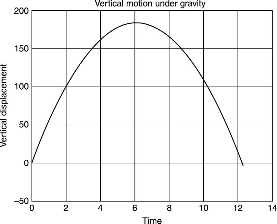
FIGURE 2.1 Distance-time graph of a stone thrown vertically upward.

This plan may seem trivial and a waste of time to write down. Yet you would be surprised how many beginners, preferring to rush straight to the computer, start with step 2 instead of step 1. It is well worth developing the mental discipline of structure-planning your program first. You can even use cut and paste to plan as follows:

1. Type the structure plan into the Editor (each line preceded by % as shown above).

2. Paste a second copy of the plan directly below the first.

3. Translate each line in the second copy into a MATLAB statement or statements (add % comments as in the example below).

4. Finally, paste all the translated MATLAB statements into the Command Window and run them (or you can just click on the green triangle in the toolbar of the Editor to execute your script).

5. If necessary, go back to the Editor to make corrections and repaste the corrected statements to the Command Window (or save the program in the Editor as an M-file and execute it).

You might like to try this as an exercise before looking at the final program, which is as follows:

% Vertical motion under gravity

g = 9.81; % acceleration due

% to gravity

u = 60; % initial velocity in

% metres/sec

t = 0 : 0.01 : 12.3; % time in seconds

s = u * t - g / 2 * t .^ 2; % vertical displacement

% in metres

plot(t, s,'k','LineWidth',3)

title( 'Vertical motion under gravity' )

xlabel( 'time' ), ylabel( 'vertical displacement' )

grid

The graphical output is shown in Figure 2.1.

Note the following points:

■ Anything in a line following the symbol % is ignored by MATLAB and may be used as a comment (description).

■ The statement t = 0 : 0.1 : 12.3 sets up a vector.

■ The formula for s is evaluated for every element of the vector t, making another vector.

■ The expression t.^2 squares each element in t. This is called an array operation and is different from squaring the vector itself, which is a matrix operation, as we will see later.

■ More than one statement can be entered on the same line if the statements are separated by commas.

■ A statement or group of statements can be continued to the next line with an ellipsis of three or more dots (...).

■ The statement disp([t' s']) first transposes the row vectors t and s into two columns and constructs a matrix from them, which is then displayed.

You might want to save the program under a helpful name, like throw.m, if you think you might come back to it. In that case, it would be worth keeping the structure plan as part of the file; just insert % symbols in front of each line. This way, the plan reminds you what the program does when you look at it again after some months. Note that you can use the context menu in the Editor to Comment/Uncomment a block of selected text. After you block selected text, right-click to see the context menu. To comment the text, scroll down to Comment, point, and click.

2.5. Operators, expressions, and statements

Any program worth its salt actually does something. What it basically does is evaluate expressions, such as

u*t - g/2*t.^2

and execute (carry out) statements, such as

balance = balance + interest

MATLAB is described as an expression based language because it interprets and evaluates typed expressions. Expressions are constructed from a variety of things, such as numbers, variables, and operators. First we need to look at numbers.

2.5.1. Numbers

Numbers can be represented in MATLAB in the usual decimal form (fixed point) with an optional decimal point,

1.2345 -123 .0001

They may also be represented in scientific notation. For example, may be represented in MATLAB as 1.2345e9. This is also called floating-point notation. The number has two parts: the mantissa, which may have an optional decimal point (1.2345 in this example) and the exponent (9), which must be an integer (signed or unsigned). Mantissa and exponent must be separated by the letter e (or E). The mantissa is multiplied by the power of 10 indicated by the exponent.

Note that the following is not scientific notation: 1.2345*10^9. It is actually an expression involving two arithmetic operations (* and ^) and therefore more time consuming. Use scientific notation if the numbers are very small or very large, since there's less chance of making a mistake (e.g., represent 0.000000001 as 1e-9).

On computers using standard floating-point arithmetic, numbers are represented to approximately 16 significant decimal digits. The relative accuracy of numbers is given by the function eps, which is defined as the distance between 1.0 and the next largest floating-point number. Enter eps to see its value on your computer.

The range of numbers is roughly to . Precise values for your computer are returned by the MATLAB functions realmin and realmax.

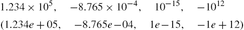
As an exercise, enter the following numbers at the command prompt in scientific notation (answers follow in parentheses):

2.5.2. Data types

MATLAB has more than a dozen fundamental data types (or classes). The default numeric data type is double precision; all MATLAB computations are in double precision. More information on data types can be found in the Help index.

MATLAB also supports signed and unsigned integer types and single-precision floating-point, by means of functions such as int8, uint8, single, and the like. However, before mathematical operations can be performed on such types, they must be converted to double precision using the double function.

2.5.3. Arithmetic operators

The evaluation of expressions is achieved by means of arithmetic operators. The arithmetic operations on two scalar constants or variables are shown in Table 2.1. Operators operate on operands (a and b in the table).

Table 2.1

Arithmetic Operations Between Two Scalars

Left division seems a little curious: Divide the right operand by the left operand. For scalar operands the expressions 1/3 and 3\1 have the same numerical value (a colleague of mine speaks of the latter as “3 under 1”). However, matrix left division has an entirely different meaning, as we will see later.

2.5.4. Operator precedence

Several operations may be combined in one expression—for example, g*t^2. MATLAB has strict precedence rules for which operations are performed first in such cases. The precedence rules for the operators in Table 2.1 are shown in Table 2.2. Note that parentheses have the highest precedence. Note also the difference between parentheses and square brackets. The former are used to alter the precedence of operators and to denote subscripts, while the latter are used to create vectors.

Table 2.2

Precedence of Arithmetic Operations

When operators in an expression have the same precedence, the operations are carried out from left to right. So a / b * c is evaluated as (a / b) * c and not as a / (b * c).

Exercises

2.1 Evaluate the following MATLAB expressions yourself before checking the answers in MATLAB:

1 + 2 * 3

4 / 2 * 2

1 + 2 / 4

1 + 2 \ 4

2 * 2 ^ 3

2 * 3 \ 3

2 ^ (1 + 2)/3

1/2e-1

2.2 Use MATLAB to evaluate the following expressions. Answers are in parentheses.

(a) (0.1667)

(b)  (64)

(c) (0.0252; use scientific or floating-point notation)

2.5.5. The colon operator

The colon operator has a lower precedence than the plus operator, as the following shows:

1+1:5

The addition is carried out first and a vector with elements 2, … , 5 is then initialized.

You may be surprised at the following:

1+[1:5]

Were you? The value 1 is added to each element of the vector 1:5. In this context, the addition is called an array operation because it operates on each element of the vector (array). Array operations are discussed below.

See Appendix B for a complete list of MATLAB operators and their precedences.

2.5.6. The transpose operator

The transpose operator has the highest precedence. Try

1:5'

The 5 is transposed first (into itself since it is a scalar!), and then a row vector is formed. Use square brackets if you want to transpose the whole vector:

[1:5]'

2.5.7. Arithmetic operations on arrays

Enter the following statements at the command line:

a = [2 4 5];

b = [6 2 2];

a .* b

a ./ b

MATLAB has four additional arithmetic operators, as shown in Table 2.3 that work on corresponding elements of arrays with equal dimensions. They are sometimes called array or element-by-element operations because they are performed element by element. For example, a .* b results in the following vector (sometimes called the array product):

[a(1)*b(1) a(2)*b(2) a(3)*b(3)]

that is, [12 8 10].

Table 2.3

Arithmetic Operators That Operate Element-by-Element on Arrays

You will have seen that a ./ b gives element-by-element division. Now try [2 3 4] .^ [4 3 1]. The ith element of the first vector is raised to the power of the ith element of the second vector. The period (dot) is necessary for the array operations of multiplication, division, and exponentiation because these operations are defined differently for matrices; they are then called matrix operations (see Chapter 6). With a and b as defined above, try a + b and a - b. For addition and subtraction, array operations and matrix operations are the same, so we don't need the period to distinguish them.

When array operations are applied to two vectors, both vectors must be the same size!

Array operations also apply between a scalar and a nonscalar. Check this with 3 .* a and a .^ 2. This property is called scalar expansion. Multiplication and division operations between scalars and nonscalars can be written with or without the period (i.e., if a is a vector, 3 .* a is the same as 3 * a).

A common application of element-by-element multiplication is finding the scalar product (also called the dot product) of two vectors x and y, which is defined as

The MATLAB function sum(z) finds the sum of the elements of the vector z, so the statement sum(a .* b) will find the scalar product of a and b (30 for a and b defined above).

Exercises

Use MATLAB array operations to do the following:

2.1. Add 1 to each element of the vector [2 3 -1].

2.2. Multiply each element of the vector [1 4 8] by 3.

2.3. Find the array product of the two vectors [1 2 3] and [0 -1 1]. (Answer: [0 -2 3])

2.4. Square each element of the vector [2 3 1].

2.5.8. Expressions

An expression is a formula consisting of variables, numbers, operators, and function names. It is evaluated when you enter it at the MATLAB prompt. For example, evaluate 2π as follows:

2 * pi

MATLAB's response is

ans =

6.2832

Note that MATLAB uses the function ans (which stands for answer) to return the last expression to be evaluated but not assigned to a variable.

If an expression is terminated with a semicolon (;), its value is not displayed, although it is still returned by ans.

2.5.9. Statements

MATLAB statements are frequently of the form

as in

s = u * t - g / 2 * t .^ 2;

This is an example of an assignment statement because the value of the expression on the right is assigned to the variable (s) on the left. Assignment always works in this direction. Note that the object on the left-hand side of the assignment must be a variable name. A common mistake is to get the statement the wrong way around, as in

a + b = c

Basically any line that you enter in the Command Window or in a program, which MATLAB accepts, is a statement, so a statement can be an assignment, a command, or simply an expression, such as

x = 29; % assignment

clear % command

pi/2 % expression

This naming convention is in keeping with most programming languages and serves to emphasize the different types of statements that are found in programming. However, the MATLAB documentation tends to refer to all of these as “functions.”

As we have seen, a semicolon at the end of an assignment or expression suppresses any output. This is useful for suppressing irritating output of intermediate results (or large matrices).

A statement that is too long to fit on one line may be continued to the next line with an ellipsis of at least three dots:

x = 3 * 4 - 8 ....

/ 2 ^ 2;

Statements on the same line may be separated by commas (output not suppressed) or semicolons (output suppressed):

a = 2; b = 3, c = 4;

Note that the commas and semicolons are not technically part of the statements; they are separators.

Statements may involve array operations, in which case the variable on the left-hand side may become a vector or a matrix.

2.5.10. Statements, commands, and functions

The distinction between MATLAB statements, commands, and functions can be a little fuzzy, since all can be entered on the command line. However, it is helpful to think of commands as changing the general environment in some way, for example, load, save, and clear. Statements do the sort of thing we usually associate with programming, such as evaluating expressions and carrying out assignments, making decisions (if), and repeating (for). Functions return with calculated values or perform some operation on data, such as sin and plot.

2.5.11. Formula vectorization

With array operations, you can easily evaluate a formula repeatedly for a large set of data. This is one of MATLAB's most useful and powerful features, and you should always look for ways to exploit it.

Let us again consider, as an example, the calculation of compound interest. An amount of money A invested over a period of years n with an annual interest rate r grows to an amount . Suppose we want to calculate final balances for investments of $750, $1000, $3000, $5000, and $11,999 over 10 years with an interest rate of 9%. The following program (comp.m) uses array operations on a vector of initial investments to do this:

format bank

A = [750 1000 3000 5000 11999];

r = 0.09;

n = 10;

B = A * (1 + r) ^ n;

disp( [A' B'] )

The output is

750.00 1775.52

1000.00 2367.36

3000.00 7102.09

5000.00 11836.82

11999.00 28406.00

Note the following:

■ In the statement B = A * (1 + r) ^ n, the expression (1 + r) ^ n is evaluated first because exponentiation has a higher precedence than multiplication.

■ Each element of the vector A is then multiplied by the scalar (1 + r) ^ n (scalar expansion).

■ The operator * may be used instead of .* because the multiplication is between a scalar and a nonscalar (although .* would not cause an error because a scalar is a special case of an array).

■ A table is displayed whose columns are given by the transposes of A and B.

This process is called formula vectorization. The operation in the statement described in bullet item 1 is such that every element in the vector B is determined by operating on every element of vector A all at once, by interpreting once a single command line.

See if you can adjust the program comp.m to find the balances for a single amount A ($1000) over 1, 5, 10, 15, and 20 years. (Hint: use a vector for n: [1 5 10 15 20].)

Exercises

2.1 Evaluate the following expressions yourself (before you use MATLAB to check). The numerical answers are in parentheses.

(a) 2 / 2 * 3 (3)

(b) 2 / 3 ̂ 2 (2/9)

(c) (2 / 3) ̂ 2 (4/9)

(d) 2 + 3 * 4 - 4 (10)

(e) 2 ̂ 2 * 3 / 4 + 3 (6)

(f) 2 ̂ (2 * 3) / (4 + 3) (64/7)

(g) 2 * 3 + 4 (10)

(h) 2 ̂ 3 ̂ 2 (64)

(i) - 4 ̂ 2 (-16; ̂ has higher precedence than -)

2.2 Use MATLAB to evaluate the following expressions. The answers are in parentheses.

(a)  (1.4142; use sqrt or ̂0.5)

(b)

(c) Find the sum of 5 and 3 divided by their product (0.5333)

(d)  (512)

(e) Find the square of 2π (39.4784; use pi)

(f)  (19.7392)

(g)  (0.3989)

(h)  (0.2821)

(i) Find the cube root of the product of 2.3 and 4.5 (2.1793)

(j)  (0.2)

(k)  (2107.2—for example, $1000 deposited for 5 years at 15% per year, with the interest compounded monthly)

(l)  (; use scientific notation—for example, 1.23e-5 … ; do not use ̂)

2.3 Try to avoid using unnecessary parentheses in an expression. Can you spot the errors in the following expression? (Test your corrected version with MATLAB.)

(2(3+4)/(5*(6+1))^2

Note that the MATLAB Editor has two useful ways of dealing with the problem of “unbalanced delimiters” (which you should know about if you have been working through Help!):

■ When you type a closing delimiter, that is, a right ), ], or }, its matching opening delimiter is briefly highlighted. So if you don't see the highlighting when you type a right delimiter, you immediately know you've got one too many.

■ When you position the cursor anywhere inside a pair of delimiters and select Text → Balance Delimiters (or press Ctrl+B), the characters inside the delimiters are highlighted.

2.4 Set up a vector n with elements 1, 2, 3, 4, 5. Use MATLAB array operations on it to set up the following four vectors, each with five elements:

(a) 2, 4, 6, 8, 10

(b) 1/2, 1, 3/2, 2, 5/2

(c) 1, 1/2, 1/3, 1/4, 1/5

(d)

2.5 Suppose vectors a and b are defined as follows:

a = [2 -1 5 0];

b = [3 2 -1 4];

Evaluate by hand the vector c in the following statements. Check your answers with MATLAB.

(a) c = a - b;

(b) c = b + a - 3;

(c) c = 2 * a + a .̂ b;

(d) c = b ./ a;

(e) c = b . a;

(f) c = a .̂ b;

(g) c = 2.̂b+a;

(h) c = 2*b/3.*a;

(i) c = b*2.*a;

2.6 Water freezes at 32° and boils at 212° on the Fahrenheit scale. If C and F are Celsius and Fahrenheit temperatures, the formula

converts from one to the other. Use the MATLAB command line to convert Celsius 37° (normal human temperature) to Fahrenheit (98.6°).

2.7 Engineers often have to convert from one unit of measurement to another, which can be tricky sometimes. You need to think through the process carefully. For example, convert 5 acres to hectares, given that an acre is 4840 square yards, a yard is 36 inches, an inch is 2.54 centimeters, and a hectare is 10,000 square meters. The best approach is to develop a formula to convert x acres to hectares. You can do this as follows.

■ One square yard

■ So one acre

=0.4047 hectares

■ So x acres hectares

Once you have found the formula (but not before), MATLAB can do the rest:

x = 5; % acres

h = 0.4047 * x; % hectares

disp( h )

2.8 Develop formulae for the following conversions, and use some MATLAB statements to find the answers (in parentheses).

(a) Convert 22 yards (an imperial cricket pitch) to meters. (20.117 meters)

(b) One pound (weight) = 454 grams. Convert 75 kilograms to pounds. (165.20 pounds)

(c) Convert 49 meters/second (terminal velocity for a falling human-shaped object) to kilometers per hour. (176.4 kilometers per hour)

(d) One atmosphere pressure = 14.7 pounds per square inch (psi) = 101.325 kilo Pascals (kPa). Convert 40 psi to kPa. (275.71 kPa)

(e) One calorie = 4.184 joules. Convert 6.25 kilojoules to calories. (1.494 kilocalories)

2.6. Output

There are two straightforward ways of getting output from MATLAB:

■ Entering a variable name, assignment, or expression on the command line, without a semicolon

■ Using the disp statement (e.g., disp( x ))

2.6.1. The disp statement

The general form of disp for a numeric variable is

disp( variable }

When you use disp, the variable name is not displayed, and you don't get a line feed before the value is displayed, as you do when you enter a variable name on the command line without a semicolon. disp generally gives a neater display.

You can also use disp to display a message enclosed in apostrophes (called a string). Apostrophes that are part of the message must be repeated:

disp( 'Pilate said, ''What is truth?''' );

To display a message and a value on the same line, use the following trick:

x = 2;

disp( ['The answer is ', num2str(x)] );

The output should be

The answer is 2

Square brackets create a vector, as we have seen. If we want to display a string, we create it; that is, we type a message between apostrophes. This we have done already in the above example by defining the string 'The answer is '. Note that the last space before the second apostrophe is part of the string. All the components of a MATLAB array must be either numbers or strings (unless you use a cell array—see Chapter 10), so we convert the number x to its string representation with the function num2str; read this as “number to string.”

You can display more than one number on a line as follows:

disp( [x y z] )

The square brackets create a vector with three elements, which are all displayed.

The command more on enables paging of output. This is very useful when displaying large matrices, for example, rand(100000,7) (see help more for details). If you forget to switch on more before displaying a huge matrix, you can always stop the display with Ctrl+C.

As you gain experience with MATLAB you may wish to learn more about the input and output capabilities in MATLAB. You can begin your search for information by clicking the question mark at the top of the desktop to open the help documents. Then search for fopen, a utility which allows you to open a file. Scroll to the bottom of the page in the help manual on this topic and find the following list of functions: fclose, feof, ferror, fprintf, fread, fscanf, fseek, ftell, fwrite. Click on fprintf, which is a formatted output utility that is popular if you are a C-language programmer. Search for input in the help manual to learn more about this function that is used in a number of examples in this text. Of course, the simplest input of data is the assignment of values to variables in a program of commands.

2.6.2. The format command

The term format refers to how something is laid out: in this case MATLAB output. The default format in MATLAB has the following basic output rules:

■ It always attempts to display integers (whole numbers) exactly. However, if the integer is too large, it is displayed in scientific notation with five significant digits—1234567890 is displayed as 1.2346e+009 (i.e., ). Check this by first entering 123456789 at the command line and then 1234567890.

■ Numbers with decimal parts are displayed with four significant digits. If the value x is in the range , it is displayed in fixed-point form; otherwise, scientific (floating-point) notation is used, in which case the mantissa is between 1 and 9.9999 (e.g., 1000.1 is displayed as 1.0001e+003). Check this by entering the following numbers at the prompt (on separate lines): 0.0011, 0.0009, 1/3, 5/3, 2999/3, 3001/3.

You can change from the default with variations on the format command, as follows. If you want values displayed in scientific notation (floating-point form) whatever their size, enter the command

format short e

All output from subsequent disp statements will be in scientific notation, with five significant digits, until the next format command is issued. Enter this command and check it with the following values: 0.0123456, 1.23456, 123.456 (all on separate lines).

If you want more accurate output, you can use format long e. This also gives scientific notation but with 15 significant digits. Try it out on 1/7. Use format long to get fixed-point notation with 15 significant digits. Try 100/7 and pi. If you're not sure of the order of magnitude of your output you can try format short g or format long g. The g stands for “general.” MATLAB decides in each case whether to use fixed or floating point.

Use format bank for financial calculations; you get fixed point with two decimal digits (for cents). Try it on 10000/7. Suppress irritating line feeds with format compact, which gives a more compact display. format loose reverts to a more airy display. Use format hex to get hexadecimal display.

Use format rat to display a number as a rational approximation (ratio of two integers). For example, pi is displayed as 355/113, a pleasant change from the tired old 22/7. Note that even this is an approximation! Try out format rat on and e (exp(1)).

The symbols +, −, and a space are displayed for positive, negative, and zero elements of a vector or matrix after the command format +. In certain applications this is a convenient way of displaying matrices. The command format by itself reverts to the default format. You can always try help format if you're confused!

2.6.3. Scale factors

Enter the following commands (MATLAB's response is also shown).

≫ format compact

≫ x = [1e3 1 1e-4]

x =

1.0e+003 *

1.0000 0.0010 0.0000

With format short (the default) and format long, a common scale factor is applied to the whole vector if its elements are very large or very small or differ greatly in magnitude. In this example, the common scale factor is 1000, so the elements displayed must all be multiplied by it to get their proper value—for example, for the second element 1.0e+003 * 0.0010 gives 1. Taking a factor of 1000 out of the third element (1e-4) leaves 1e-7, which is represented by 0.0000 since only four decimal digits are displayed.

If you don't want a scale factor, try format bank or format short e:

≫x

x =

1000.0000 1.00 0.00

≫format short e

≫x

x =

1.0000e+003  1.0000e+000  1.0000e-004

2.7. Repeating with for

So far we have seen how to get data into a program (i.e., provide input), how to do arithmetic, and how to get some results (i.e., get output). In this section we look at a new feature: repetition. This is implemented by the extremely powerful for construct. We will first look at some examples of its use, followed by explanations.

For starters, enter the following group of statements on the command line. Enter the command format compact first to make the output neater:

for i = 1:5, disp(i), end

Now change it slightly to

for i = 1:3, disp(i), end

And what about

for i = 1:0, disp(i), end

Can you see what's happening? The disp statement is repeated five times, three times, and not at all.

2.7.1. Square roots with Newton's method

The square root x of any positive number a may be found using only the arithmetic operations of addition, subtraction, and division with Newton's method. This is an iterative (repetitive) procedure that refines an initial guess.

To introduce in a rather elementary way the notion of structured programming (to be described in more detail in Chapter 3), let us consider the structure plan of the algorithm to find a square root and a program with sample output for .

Here is the structure plan:

1. Initialize a

2. Initialize x to

3. Repeat 6 times (say) the following:

Replace x by

Display x

4. Stop

Here is the program:

a = 2;

x = a/2;

disp(['The approach to sqrt(a) for a = ', num2str(a)])

for i = 1:6

x = (x + a / x) / 2;

disp( x )

end

disp( 'Matlab''s value: ' )

disp( sqrt(2) )

Here is the output (after selecting format long):

The approach to sqrt(a) for a = 2

1.50000000000000

1.41666666666667

1.41421568627451

1.41421356237469

1.41421356237310

1.41421356237310

Matlab's value:

1.41421356237310

The value of x converges to a limit rather quickly in this case, . Note that it is identical to the value returned by MATLAB's sqrt function. Most computers and calculators use a similar method internally to compute square roots and other standard mathematical functions.

The general form of Newton's method is presented in Chapter 14.

2.7.2. Factorials!

Run the following program to generate a list of n and n! (“n factorial,” or “n shriek”), where

(2.1)

n = 10;

fact = 1;

for k = 1:n

fact = k * fact;

disp( [k fact] )

end

Experiment to find the largest value of n for which MATLAB can find the n factorial. (You had better leave out the disp statement! Or you can move it from above the end command to below it.)

2.7.3. Limit of a sequence

for loops are ideal for computing successive members of a sequence (as in Newton's method). The following example also highlights a problem that sometimes occurs when computing a limit. Consider the sequence

where a is any constant and n! is the factorial function defined above. The question is this: What is the limit of this sequence as n gets indefinitely large? Let's take the case . If we try to compute directly, we can get into trouble, because n! grows very rapidly as n increases, and numerical overflow can occur. However, the situation is neatly transformed if we spot that is related to as follows:

There are no numerical problems now.

The following program computes for and increasing values of n.

a = 10;

x = 1;

k = 20; % number of terms

for n = 1:k

x = a * x / n;

disp( [n x] )

end

2.7.4. The basic for construct

In general the most common form of the for loop (for use in a program, not on the command line) is

for index = j:k

statements;

end

or

for index = j:m:k

statements;

end

Note the following points carefully:

■ j:k is a vector with elements .

■ j:m:k is a vector with elements  , such that the last element does not exceed k if or is not less than k if .

■ index must be a variable. Each time through the loop it will contain the next element of the vector j:k or j:m:k, and statements (there may be one or more) are carried out for each of these values.

If the for construct has the form

for k = first:increment:last

The number of times the loop is executed may be calculated from the following equation:

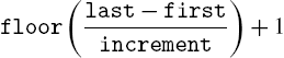
where the MATLAB function floor(x) rounds x down toward −∞. This value is called the iteration or trip count. As an example, let us consider the statement for i = 1:2:6. It has an iteration count of

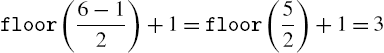
Thus i takes the values 1, 3, 5. Note that if the iteration count is negative, the loop is not executed.

■ On completion of the for loop the index contains the last value used.

■ If the vector j:k or j:m:k is empty, statements are not executed and control passes to the statement following end.

■ The index does not have to appear explicitly in statements. It is basically a counter. In fact, if the index does appear explicitly in statements, the for can often be vectorized (more details on this are given in Section 2.7.7). A simple example of a more efficient (faster) program is as follows. The examples with disp at the beginning of this section were for illustration only; strictly, it would be more efficient to say (without “for”)

i = 1:5; disp( i' )

Can you see the difference? In this case i is assigned as a vector (hence, this change vectorizes the original program).

■ It is good programming style to indent (tabulate) the statements inside a for loop. You may have noticed that the Editor does this for you automatically with a feature called smart indenting.

2.7.5. for in a single line

If you insist on using for in a single line, here is the general form:

for index = j:k; statements; end

or

for index = j:m:k; statements; end

Note the following:

■ Don't forget the commas (semicolons will also do if appropriate). If you leave them out you will get an error message.

■ Again, statements can be one or more statements separated by commas or semicolons.

■ If you leave out end, MATLAB will wait for you to enter it. Nothing will happen until you do so.

2.7.6. More general for

A more general form of for is

for index = v

where v is any vector. The index moves through each element of the vector in turn, providing a neat way of processing each item in a list. Other forms of the for loop as well as the while loop will be discussed in Chapter 8.

2.7.7. Avoid for loops by vectorizing!

There are situations where a for loop is essential, as in many of the examples in this section so far. However, given the way MATLAB has been designed, for loops tend to be inefficient in terms of computing time. If you have written a for loop that involves the index of the loop in an expression, it may be possible to vectorize the expression, making use of array operations where necessary, as the following examples show.

Suppose you want to evaluate

(and can't remember the formula for the sum). Here's how to do it with a for loop (run the program, which also times how long it takes):

t0 = clock;

s = 0;

for n = 1:100000

s = s + n;

end

etime(clock, t0)

The MATLAB function clock returns a six-element vector with the current date and time in the format year, month, day, hour, minute, seconds. Thus, t0 records when the calculation starts.

The function etime returns the time in seconds elapsed between its two arguments, which must be vectors as returned by clock. On a Pentium II, it returned about 3.35 seconds, which is the total time for this calculation. (If you have a faster PC, it should take less time.)

Now try to vectorize this calculation (before looking at the solution). Here it is:

t0 = clock;

n = 1:100000;

s = sum( n );

etime(clock, t0)

This way takes only 0.06 seconds on the same PC—more than 50 times faster!

There is a neater way of monitoring the time taken to interpret MATLAB statements: the tic and toc function. Suppose you want to evaluate

Here's the for loop version:

tic

s = 0;

for n = 1:100000

s = s + 1/n^2;

end

toc

which takes about 6 seconds on the same PC. Once again, try to vectorize the sum:

tic

n = 1:100000;

s = sum( 1./n.^2 );

toc

The same PC gives a time of about 0.05 seconds for the vectorized version—more than 100 times faster! (Of course, the computation time in these examples is small regardless of the method applied. However, learning how to improve the efficiency of computation to solve more complex scientific or engineering problems will be helpful as you develop good programming skills. More details on good problem-solving and program design practices are introduced at the end of this chapter and dealt with, in more detail, in the next.)

Series with alternating signs are a little more challenging. This series sums to (the natural logarithm of 2):

Here's how to find the sum of the first 9999 terms with a for loop (note how to handle the alternating sign):

sign = -1;

s = 0;

for n = 1:9999

sign = -sign;

s = s + sign / n;

end

Try it. You should get 0.6932. MATLAB's log(2) gives 0.6931. Not bad.

The vectorized version is as follows:

n = 1:2:9999;

s = sum( 1./n - 1./(n+1) )

If you time the two versions, you will again find that the vectorized form is many times faster.

MATLAB's functions naturally exploit vectorization wherever possible. For example, prod(1:n) will find n! much faster than the code at the beginning of this section (for large values of n).

Exercises

Write MATLAB programs to find the following sums with for loops and by vectorization. Time both versions in each case.

■  (sum is 333 833 500)

■  (sum is 0.7849—converges slowly to π/4)

■ Sum the left-hand side of the series

2.8. Decisions

The MATLAB function rand generates a random number in the range 0–1. Enter the following two statements at the command line:

r = rand

if r > 0.5 disp( 'greater indeed' ), end

MATLAB should only display the message greater indeed if r is in fact greater than 0.5 (check by displaying r). Repeat a few times—cut and paste from the Command History window (make sure that a new r is generated each time).

As a slightly different but related exercise, enter the following logical expression on the command line:

2 > 0

Now enter the logical expression -1 > 0. MATLAB gives a value of 1 to a logical expression that is true and 0 to one that is false.

2.8.1. The one-line if statement

In the last example MATLAB has to make a decision; it must decide whether or not r is greater than 0.5. The if construct, which is fundamental to all computing languages, is the basis of such decision making. The simplest form of if in a single line is

if condition; statements; end

Note the following points:

■ condition is usually a logical expression (i.e., it contains a relational operator), which is either true or false. The relational operators are shown in Table 2.4. MATLAB allows you to use an arithmetic expression for condition. If the expression evaluates to 0, it is regarded as false; any other value is true. This is not generally recommended; the if statement is easier to understand (for you or a reader of your code) if condition is a logical expression.

Table 2.4

Relational Operators

■ If condition is true, statement is executed, but if condition is false, nothing happens.

■ condition may be a vector or a matrix, in which case it is true only if all of its elements are nonzero. A single zero element in a vector or matrix renders it false.

if condition statement, end

Here are more examples of logical expressions involving relational operators, with their meanings in parentheses:

b^2 < 4*a*c (b² < 4ac)

x >= 0 (x ⩾ 0)

a ~= 0(a ≠ 0)

b^2 == 4*a*c (b² = 4ac)

Remember to use the double equal sign (==) when testing for equality:

if x == 0; disp( 'x equals zero'); end

Exercises

The following statements all assign logical expressions to the variable x. See if you can correctly determine the value of x in each case before checking your answer with MATLAB.

(a) x = 3 > 2

(b) x = 2 > 3

(c) x = -4 <= -3

(d) x = 1 < 1

(e) x = 2 ~= 2

(f) x = 3 == 3

(g) x = 0 < 0.5 < 1

Did you get item (f)? 3 == 3 is a logical expression that is true since 3 is undoubtedly equal to 3. The value 1 (for true) is therefore assigned to x. After executing these commands type the command whos to find that the variable x is in the class of logical variables.

What about (g)? As a mathematical inequality,

is undoubtedly true from a nonoperational point of view. However, as a MATLAB operational expression, the left-hand < is evaluated first, 0 < 0.5, giving 1 (true). Then the right-hand operation is performed, 1 < 1, giving 0 (false). Makes you think, doesn't it?

2.8.2. The if-else construct

If you enter the two lines

x = 2;

if x < 0 disp( 'neg' ), else disp( 'non-neg'), end

do you get the message non-neg? If you change the value of x to −1 and execute the if again, do you get the message neg this time? Finally, if you try

if 79 disp( 'true' ), else disp('false' ), end

do you get true? Try other values, including 0 and some negative values.

Most banks offer differential interest rates. Suppose the rate is 9% if the amount in your savings account is less than $5000, but 12% otherwise. The Random Bank goes one step further and gives you a random amount in your account to start with! Run the following program a few times:

bal = 10000 * rand;

if bal < 5000

rate = 0.09;

else

rate = 0.12;

end

newbal = bal + rate * bal;

disp( 'New balance after interest compounded is:' )

format bank

disp( newbal )

Display the values of bal and rate each time from the command line to check that MATLAB has chosen the correct interest rate.

The basic form of if-else for use in a program file is

if condition

statementsA

else

statementsB

end

Note that

■ statementsA and statementsB represent one or more statements.

■ If condition is true, statementsA are executed, but if condition is false, statementsB are executed. This is essentially how you force MATLAB to choose between two alternatives.

■ else is optional.

2.8.3. The one-line if-else statement

The simplest general form of if-else for use on one line is

if condition; statementA; else; statementB; end

Note the following:

■ Commas (or semicolons) are essential between the various clauses.

■ else is optional.

■ end is mandatory; without it, MATLAB will wait forever.

2.8.4. elseif

Suppose the Random Bank now offers 9% interest on balances of less than $5000, 12% for balances of $5000 or more but less than $10,000, and 15% for balances of $10,000 or more. The following program calculates a customer's new balance after one year according to this scheme:

bal = 15000 * rand;

if bal < 5000

rate = 0.09;

elseif bal < 10000

rate = 0.12;

else

rate = 0.15;

end

newbal = bal + rate * bal;

format bank

disp( 'New balance is:' )

disp( newbal )

Run the program a few times, and once again display the values of bal and rate each time to convince yourself that MATLAB has chosen the correct interest rate.

In general, the elseif clause is used:

if condition1

statementsA

elseif condition2

statementsB

elseif condition3

statementsC

...

else

statementsE

end

This is sometimes called an elseif ladder. It works as follows:

1. condition1 is tested. If it is true, statementsA are executed; MATLAB then moves to the next statement after end.

2. If condition1 is false, MATLAB checks condition2. If it is true, statementsB are executed, followed by the statement after end.

3. In this way, all conditions are tested until a true one is found. As soon as a true condition is found, no further elseifs are examined and MATLAB jumps off the ladder.

4. If none of the conditions is true, statements after else are executed.

5. Arrange the logic so that not more than one of the conditions is true.

6. There can be any number of elseifs, but at most one else.

7. elseif must be written as one word.

8. It is good programming style to indent each group of statements as shown.

2.8.5. Logical operators

More complicated logical expressions can be constructed using the three logical operators: & (and), | (or), and ~ (not). For example, the quadratic equation

has equal roots, given by , provided that and (Figure 2.2). This translates into the following MATLAB statements:

if (b ^ 2 - 4*a*c == 0) & (a ~= 0)

x = -b / (2*a);

end

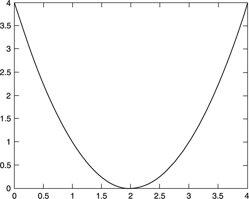
FIGURE 2.2 Quadratic function with equal roots.

Of course, a, b, and c must be assigned values prior to reaching this set of statements. Note the double equal sign in the test for equality; see Chapter 5 for more on logical operators.

2.8.6. Multiple ifs versus elseif

You could have written the Random Bank program as follows:

bal = 15000 * rand;

if bal < 5000

rate = 0.09;

end

if bal >= 5000 & bal < 10000

rate = 0.12;

end

if bal >= 10000

rate = 0.15;

end

newbal = bal + rate * bal;

format bank

disp( 'New balance is' )

disp( newbal )

However, this is inefficient since each of the three conditions is always tested, even if the first one is true. In the earlier elseif version, MATLAB jumps off the elseif ladder as soon as it finds a true condition. This saves a lot of computing time (and is easier to read) if the if construct is in a loop that is repeated often.

Using this form, instead of the elseif ladder, you can make the following common mistake:

if bal < 5000

rate = 0.09;

end

if bal < 10000

rate = 0.12;

end

if bal >= 10000

rate = 0.15;

end

Can you see why you get the wrong answer (1120 instead of 1090) if bal has the value 1000? When designing the logic, you need to make sure that one and only one of the conditions will be true at any one time.

Another mistake frequently made is to replace the second if with something like

if 5000 < bal < 10000

rate = 0.12;

end

which is compelling, as we saw above. However, whatever the value of bal, this condition will always be true. Can you see why? (Note that if bal is greater than 5000—for example, bal = 20000—the numerical truth value of the first test, namely, 5000 < bal, is true and hence has the numerical value of 1 since 1 is always less than 10000, even if bal = 20000.)

2.8.7. Nested ifs

An if construct can contain further ifs and so on. This is called nesting and should not be confused with the elseif ladder. You have to be careful with elses. In general, else belongs to the most recent if that has not been ended. The correct positioning of end is therefore very important, as the next example demonstrates.

Suppose you want to compute the solution to a quadratic equation. You may want to check whether to prevent a division by zero. Your program could contain the following nested ifs:

...

d = b ^ 2 - 4*a*c;

if a ~= 0

if d < 0

disp( 'Complex roots' )

else

x1 = (-b + sqrt( d )) / (2*a);

x2 = (-b - sqrt( d )) / (2*a);

end % first end <<<<<<<<<<<<

end

The else belongs to the second if by default, as intended.

Now move the first end up as follows:

d = b ^ 2 {-} 4*a*c;

if a $^\sim$= 0

if d < 0

disp( 'Complex roots' )

end \% first end moved up now <<<<<<<<<<<<

else

x1 = (-b + sqrt( d )) / (2*a);

x2 = (-b {-} sqrt( d )) / (2*a);

end

The end that has been moved now closes the second if. The result is that else belongs to the first if instead of to the second one. Division by zero is therefore guaranteed instead of prevented!

2.8.8. Vectorizing ifs?

You may be wondering if for statements enclosing ifs can be vectorized. The answer is yes, courtesy of logical arrays. Discussion of this rather interesting topic is postponed until Chapter 5.

2.8.9. The switch statement

switch executes certain statements based on the value of a variable or expression. In this example it is used to decide whether a random integer is 1, 2, or 3 (see Section 5.1.5 for an explanation of this use of rand):

d = floor(3*rand) + 1

switch d

case 1

disp( 'That''s a 1!' );

case 2

disp( 'That''s a 2!' );

otherwise

disp( 'Must be 3!' );

end

Multiple expressions can be handled in a single case statement by enclosing the case expression in a cell array (see Chapter 10):

d = floor(10*rand);

switch d

case {2, 4, 6, 8}

disp( 'Even' );

case {1, 3, 5, 7, 9}

disp( 'Odd' );

otherwise

disp( 'Zero' );

end

2.9. Complex numbers

If you are not familiar with complex numbers, you can safely skip this section. However, it is useful to know what they are since the square root of a negative number may come up as a mistake if you are trying to work only with real numbers.

It is very easy to handle complex numbers in MATLAB. The special values i and j stand for . Try sqrt(-1) to see how MATLAB represents complex numbers.

The symbol i may be used to assign complex values, for example,

z = 2 + 3*i

represents the complex number (real part 2, imaginary part 3). You can also input a complex value like this:

2 + 3*i

in response to the input prompt (remember, no semicolon). The imaginary part of a complex number may also be entered without an asterisk, 3i.

All of the arithmetic operators (and most functions) work with complex numbers, such as sqrt(2 + 3*i) and exp(i*pi). Some functions are specific to complex numbers. If z is a complex number, real(z), imag(z), conj(z), and abs(z) all have the obvious meanings.

A complex number may be represented in polar coordinates:

angle(z) returns θ between −π and π; that is, atan2(imag(z), real(z)). abs(z) returns the magnitude r.

Since gives the unit circle in polars, complex numbers provide a neat way of plotting a circle. Try the following:

circle = exp( 2*i*[1:360]*pi/360 );

plot(circle)

axis('equal')

Note these points:

■ If y is complex, the statement plot(y) is equivalent to

plot(real(y), imag(y))

■ The statement axis('equal') is necessary to make circles look round; it changes what is known as the aspect ratio of the monitor. axis('normal') gives the default aspect ratio.

If you are using complex numbers, be careful not to use i or j for other variables; the new values will replace the value of and will cause nasty problems.

For complex matrices, the operations ' and .' behave differently.  The ' operator is the complex conjugate transpose, meaning rows and columns are interchanged and signs of imaginary parts are changed. The .' operator, on the other hand, does a pure transpose without taking the complex conjugate. To see this, set up a complex matrix a with the statement

a = [1+i 2+2i; 3+3i 4+4i]

which results in

a =

1.0000 + 1.0000i 2.0000 + 2.0000i

3.0000 + 3.0000i 4.0000 + 4.0000i

The statement

a'

then results in the complex conjugate transpose

ans =

1.0000 - 1.0000i 3.0000 - 3.0000i

2.0000 - 2.0000i 4.0000 - 4.0000i

whereas the statement

a.'

results in the pure transpose

ans =

1.0000 + 1.0000i 3.0000 + 3.0000i

2.0000 + 2.0000i 4.0000 + 4.0000i

Summary

■ The MATLAB desktop consists of a number of tools: the Command Window, the Workspace browser, the Current Directory browser, and the Command History window.

■ MATLAB has a comprehensive online Help system. It can be accessed through the Help button (?) on the desktop toolbar or the Help menu in any tool.

■ A MATLAB program can be written in the Editor and cut and pasted to the Command Window (or it can be executed from the editor by clicking the green right arrow in the toolbar at the top of the Editor window).

■ A script file is a text file (created by the MATLAB Editor or any other text editor) containing a collection of MATLAB statements. In other words, it is a program. The statements are carried out when the script file name is entered at the prompt in the Command Window. A script file name must have the .m extension. Script files are therefore also called M-files.

■ The recommended way to run a script is from the Current Directory browser. The output from the script will then appear in the Command Window.

■ A variable name consists only of letters, digits, and underscores, and must start with a letter. Only the first 63 characters are significant. MATLAB is case-sensitive by default. All variables created during a session remain in the workspace until removed with clear. The command who lists the variables in the workspace; whos gives their sizes.

■ MATLAB refers to all variables as arrays, whether they are scalars (single-valued arrays), vectors, (1D arrays), or matrices (2D arrays).

■ MATLAB names are case-sensitive.

■ The Workspace browser on the desktop provides a handy visual representation of the workspace. Clicking a variable in it invokes the Array Editor, which may be used to view and change variable values.

■ Vectors and matrices are entered in square brackets. Elements are separated by spaces or commas. Rows are separated by semicolons. The colon operator is used to generate vectors, with elements increasing (decreasing) by regular increments (decrements). Vectors are row vectors by default. Use the apostrophe transpose operator (') to change a row vector into a column vector.

■ An element of a vector is referred to by a subscript in parentheses. A subscript may itself be a vector. Subscripts always start at 1.

■ The diary command copies everything that subsequently appears in the Command Window to the specified text file until the command diary off is given.

■ Statements on the same line may be separated by commas or semicolons.

■ A statement may be continued to the next line with an ellipsis of at least three dots.

■ Numbers may be represented in fixed-point decimal notation or in floating-point scientific notation.

■ MATLAB has 14 data types. The default numeric type is double precision. All mathematical operations are carried out in double precision.

■ The six arithmetic operators for scalars are +, -, *, \, /, and ^. They operate according to rules of precedence.

■ An expression is a rule for evaluating a formula using numbers, operators, variables, and functions. A semicolon after an expression suppresses display of its value.

■ Array operations are element by element between vectors or between scalars and vectors. The array operations of multiplication, right and left division, and exponentiation are indicated by .*, ./, .\, and .^ to distinguish them from vector and matrix operations of the same name. They may be used to evaluate a formula repeatedly for some or all of the elements of a vector. This is called vectorization of the formula.

■ disp is used to output (display) numbers and strings. num2str is useful with disp for displaying strings and numbers on the same line.

■ The format command controls the way output is displayed.

■ When vectors are displayed, a common scale factor is used if the elements are very large or very small, or differ greatly in magnitude.

■ The for statement is used to repeat a group of statements a fixed number of times. If the index of a for statement is used in the expression being repeated, the expression can often be vectorized, saving a great deal of computing time.

■ tic and toc may be used as a stopwatch.

■ Logical expressions have the value true (1) or false (0) and are constructed with the six relational operators >, >=, <, <=, ==, and ~=. Any expression that evaluates to zero is regarded as false. Any other value is true. More complicated logical expressions can be formed from other logical expressions using the logical operators & (and), | (or), and ~ (not).

■ if–else executes different groups of statements according to whether a logical expression is true or false. The elseif ladder is a good way to choose between a number of options, only one of which should be true at a time.

■ switch enables choices to be made between discrete cases of a variable or expression.

■ A string is a collection of characters enclosed in apostrophes.

■ Complex numbers may be represented using the special variables i and j, which stand for the unit imaginary number .

Exercises

2.1 Decide which of the following numbers are not acceptable in MATLAB, and state why:

(a) 9,87

(b) .0

(c) 25.82

(d) -356231

(e) 3.57*e2

(f) 3.57e2.1

(g) 3.57e+2

(h) 3,57e-2

2.2 State, giving reasons, which of the following are not valid MATLAB variable names:

(a) a2

(b) a.2

(c) 2a

(d) 'a'one

(e) aone

(f) _x_1

(g) miXedUp

(h) pay day

(i) inf

(j) Pay_Day

(k) min*2

(l) what

2.3 Translate the following expressions into MATLAB:

(a)

(b)

(c)

(d)

(e)

(f)

(g)

(h)

2.4 Translate the following into MATLAB statements:

(a) Add 1 to the value of i and store the result in i.

(b) Cube i, add j to this, and store the result in i.

(c) Set g equal to the larger of the two variables e and f.

(d) If d is greater than 0, set x equal to −b.

(e) Divide the sum of a and b by the product of c and d, and store the result in x.

2.5 What's wrong with the following MATLAB statements?

(a) n + 1 = n;

(b) Fahrenheit temp = 9*C/5 + 32;

(c) 2 = x;

2.6 Write a program to calculate x, where

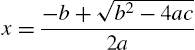
and , ,  (Answer 3.0)

2.7 There are eight pints in a gallon and 1.76 pints in a liter. The volume of a tank is given as 2 gallons and 4 pints. Write a script that inputs this volume in gallons and pints and converts it to liters. (Answer: 11.36)

2.8 Write a program to calculate gasoline consumption. It should assign the distance traveled (in kilometers) and the amount of gas used (in liters) and compute the consumption in km/liter as well as in the more usual form of liters/100 km. Write some helpful headings so that your output looks something like this:

Distance Liters used km/L L/100km

528 46.23 11.42 8.76

2.9 Write some statements in MATLAB that exchange the contents of two variables a and b, using only one additional variable t.

2.10 Try Exercise 2.9 without using any additional variables!

2.11 If C and F are Celsius and Fahrenheit temperatures, respectively, the formula for conversion from Celsius to Fahrenheit is .

(a) Write a script that will ask you for the Celsius temperature and display the Fahrenheit equivalent with some sort of comment, such as

The Fahrenheit temperature is:...

Try it out on the following Celsius temperatures (answers in parentheses): 0 (32), 100 (212), −40 (−40!), 37 (normal human temperature: 98.6).

(b) Change the script to use vectors and array operations to compute the Fahrenheit equivalents of Celsius temperatures ranging from to in steps of , and display them in two columns with a heading, like this:

Celsius Fahrenheit

20.00 68.00

21.00 69.80

...

30.00 86.00

2.12 Generate a table of conversions from degrees (first column) to radians (second column). Degrees should go from to in steps of . Recall that π radians .

2.13 Set up a matrix (table) with degrees in the first column from 0 to 360 in steps of 30, sines in the second column, and cosines in the third column. Now try to add tangents in the fourth column. Can you figure out what's going on? Try some variations of the format command.

2.14 Write some statements that display a list of integers from 10 to 20 inclusive, each with its square root next to it.

2.15 Write a single statement to find and display the sum of the successive even integers 2, 4, … , 200. (Answer: 10,100)

2.16 Ten students in a class take a test. The marks are out of 10. All the marks are entered in a MATLAB vector, marks. Write a statement to find and display the average mark. Try it on the following:

5 8 0 10 3 8 5 7 9 4 (Answer: 5.9)

Hint: Use the mean function.

2.17 What are the values of x and a after the following statements have been executed?

(a) a = 0;

(b) i = 1;

(c) x = 0;

(d) a = a + i;

(e) x = x + i / a;

(f) a = a + i;

(g) x = x + i / a;

(h) a = a + i;

(i) x = x + i / a;

(j) a = a + i;

(k) x = x + i / a;

2.18 Rewrite the statements in Exercise 2.17 more economically by using a for loop. Can you do even better by vectorizing the code?

2.19 Work out by hand the output of the following script for n = 4:

n = input( 'Number of terms? ' );

s = 0;

for k = 1:n

s = s + 1 / (k ^ 2);

end;

disp(sqrt(6 * s))

If you run this script for larger and larger values of n, you will find that the output approaches a well-known limit. Can you figure out what it is? Now rewrite the script using vectors and array operations.

2.20 Work through the following script by hand. Draw up a table of the values of i, j, and m to show how they change while the script executes. Check your answers by running the script.

v = [3 1 5];

i = 1;

for j = v

i = i + 1;

if i == 3

i = i + 2;

m = i + j;

end

end

2.21 The steady-state current I flowing in a circuit that contains a resistance , capacitance , and inductance in series is given by

where and are the input voltage and angular frequency, respectively. Compute the value of I. (Answer: 0.0396)

2.22 The electricity accounts of residents in a very small town are calculated as follows:

■ If 500 units or fewer are used, the cost is 2 cents per unit.

■ If more than 500 but not more than 1000 units are used, the cost is $10 for the first 500 units and 5 cents for every unit in excess of 500.

■ If more than 1000 units are used, the cost is $35 for the first 1000 units plus 10 cents for every unit in excess of 1000.

■ A basic service fee of $5 is charged, no matter how much electricity is used.

Write a program that enters the following five consumptions into a vector and uses a for loop to calculate and display the total charge for each one: 200, 500, 700, 1000, 1500. (Answers: $9, $15, $25, $40, $90)

2.23 Suppose you deposit $50 in a bank account every month for a year. Every month, after the deposit has been made, interest at the rate of 1% is added to the balance: After one month the balance is $50.50, and after two months it is $101.51. Write a program to compute and print the balance each month for a year. Arrange the output to look something like this:

MONTH MONTH-END BALANCE

1 50.50

2 101.51

3 153.02

...

12 640.47

2.24 If you invest $1000 for one year at an interest rate of 12%, the return is $1120 at the end of the year. But if interest is compounded at the rate of 1% monthly (i.e., 1/12 of the annual rate), you get slightly more interest because it is compounded. Write a program that uses a for loop to compute the balance after a year of compounding interest in this way. The answer should be $1126.83. Evaluate the formula for this result separately as a check: .

2.25 A plumber opens a savings account with $100,000 at the beginning of January. He then makes a deposit of $1000 at the end of each month for the next 12 months (starting at the end of January). Interest is calculated and added to his account at the end of each month (before the $1000 deposit is made). The monthly interest rate depends on the amount A in his account at the time interest is calculated, in the following way:

Write a program that displays, under suitable headings, for each of the 12 months, the situation at the end of the month as follows: the number of the month, the interest rate, the amount of interest, and the new balance. (Answer: Values in the last row of output should be 12, 0.02, 2534.58, 130263.78.)

2.26 It has been suggested that the population of the United States may be modeled by the formula

where t is the date in years. Write a program to compute and display the population every ten years from 1790 to 2000. Try to plot a graph of the population against time as well (Figure 9.16 shows this graph compared with actual data). Use your program to find out if the population ever reaches a “steady state” (i.e., stops changing).

2.27 A mortgage bond (loan) of amount L is obtained to buy a house. The interest rate r is 15%. The fixed monthly payment P that will pay off the bond loan over N years is given by the formula

(a) Write a program to compute and print P if and the bond is for $50,000. You should get $658.39.

(b) See how P changes with N by running the program for different values of N (use input). Can you find a value for which the payment is less than $625?

(c) Go back to and examine the effect of different interest rates. You should see that raising the interest rate by 1% (0.01) increases the monthly payment by about $37.

2.28 It is useful to work out how the period of a bond repayment changes if you increase or decrease P. The formula for N is given by

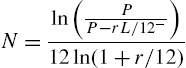
(a) Write a new program to compute this formula. Use the built-in function log for the natural logarithm ln. How long will it take to pay off a loan of $50,000 at $800 a month if the interest remains at 15%? (Answer: 10.2 years—nearly twice as fast as when paying $658 a month.)

(b) Use your program to find out by trial and error the smallest monthly payment that will pay off the loan this side of eternity. Hint: recall that it is not possible to find the logarithm of a negative number, so P must not be less than .

Appendix 2.A. Supplementary material

Supplementary material related to this chapter can be found online at http://dx.doi.org/10.1016/B978-0-08-100877-5.00003-7.