Essential MATLAB for Engineers and Scientists (2013)
PART 2
Applications
CHAPTER 16
SIMULINK® Toolbox
Abstract
The objective of this chapter is to introduce Simulink (a graphical programming environment) by applying it to solve dynamic systems investigated by science, technology, engineering, and mathematics students. The first topic covered in this chapter is the process of opening Simulink and initiating the construction of a signal processing model. Subsequently, we examine two examples of dynamic systems typically investigated by students in their first-year courses in physics. The next two dynamic systems examined are classic nonlinear equations typically investigated in courses on nonlinear dynamical systems. The examples examined in this chapter are: (1) A spring, mass damper model of a mechanical system. (2) A bouncing ball model. (3) The van der Pol oscillator. (4) The Duffing oscillator.
Keywords
Examination of oscillatory systems; Linear and nonlinear; Graphical programming; SIMULINK
CHAPTER OUTLINE
Mass-spring-damper dynamic system
Bouncing ball dynamic system
The van der Pol oscillator
The Duffing oscillator
Exercises
Supplementary material
The objective of this chapter is to introduce Simulink by applying it to solve dynamic systems investigated by science, technology, engineering and mathematics students. The first topic covered in this chapter is the process of opening Simulink and initiating the construction of a signal processing model. Subsequently, we examine two examples of dynamic systems typically investigated by students in their first-year courses in physics. The next two dynamic systems examined are classic nonlinear equations typically investigated in courses on nonlinear dynamical systems. The examples examined in this chapter are as follows:
■ An example of signal processing illustrating the initiation of the construction of a Simulink model.
■ A spring, mass damper model of a mechanical system.
■ A bouncing ball model.
■ The van der Pol oscillator.
■ The Duffing oscillator.
In this chapter an introduction to applying Simulink software via relatively simple yet interesting examples from classical mechanics is presented. In a typical science, technology, engineering and mathematics program at universities in the US the students are introduced to dynamical systems modeling in their first-year course on physics. In the first course they learn about systems that can be modeled by springs, masses and damping devices. In the second course the analogous electrical system that can be modeled by resistors, inductors and capacitors is investigated. How to simulate the dynamics of these systems with Simulink is examined in this chapter.
What is Simulink? As described in the help available with this toolbox: It is used to model, simulate and analyze dynamic systems. It enables you to pose questions about a system, model the system and observe what happens. “With Simulink, you can easily build models from scratch, or modify existing models to meet your needs. Simulink supports linear and nonlinear systems, modeled in continuous time, sampled time, or a hybrid of the two. Systems can also be multirate—having different parts that are sampled or updated at different rates.” It is a graphical programming environment.
To conclude this introduction we will examine a simple example of a signal processing model. Recall that the help files available can be opened by clicking the question mark, ‘?’, just below the word “Help” in the toolbars at the top of the MATLAB desktop. Click on Simulink to open the e-manual on this toolbox. The guidelines provided in the help for the development of more sophisticated dynamic system models provides one of the key suggestions for learning to use Simulink. It is to develop a new model by starting, if possible, with an existing model, modifying it to develop a new model to solve a new problem.
To start the exercises we need to open Simulink. This can be done by executing the following command in the command window.
>> simulink
This command opens the Simulink Start Window illustrated in Figure 16.1. Click on the Blank Model pain near the middle of the start window. A model building window illustrated in Figure 16.2 opens. Click the icon in the toolbar to open the library browser. This browser is illustrated in Figure 16.3. In the left panel of the browser an index of the Libraries is provided. Pointing and clicking on any of the items opens up the various utilities available to design (or develop) a model within Simulink to simulate a dynamic system. By single-clicking on the “white-page” icon below the word “File” just below the title of the browser window opens a new model; this is illustrated in Figure 16.3. Pull down the File menu in the untitled model window, point and click “save” and name the model that you plan to build, e.g., name it Example1. This operation creates a file named Example1.mdl. Note the file extension .mdl. This is the file extension that identifies the file as a Simulink model. The new model window with this name is illustrated in Figure 16.4. This will help save your work as you build and debug the model to solve a particular dynamic system problem.

FIGURE 16.1 Simulink window start page.

FIGURE 16.2 The Simulink untitled coding window.
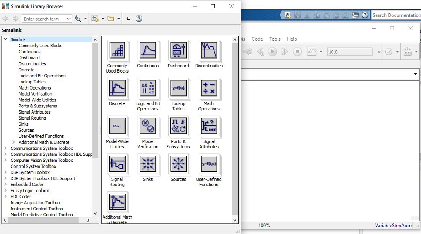
FIGURE 16.3 The Simulink library browser with the Simulink untitled coding window.

FIGURE 16.4 The untitled working window renamed “Example1”.
While in the model window hold “Ctrl” and “e” simultaneously to open the solver configuration window illustrated in Figure 16.5. Note that the default “Relative tolerance” is 1e–3, the “Solver” is ode45 among other parameters. Except for the first example below the “Relative tolerance” was changed to 1e–6. In addition, in some cases the solver applied was changed. The solver applied is also noted at the bottom right of the model window.
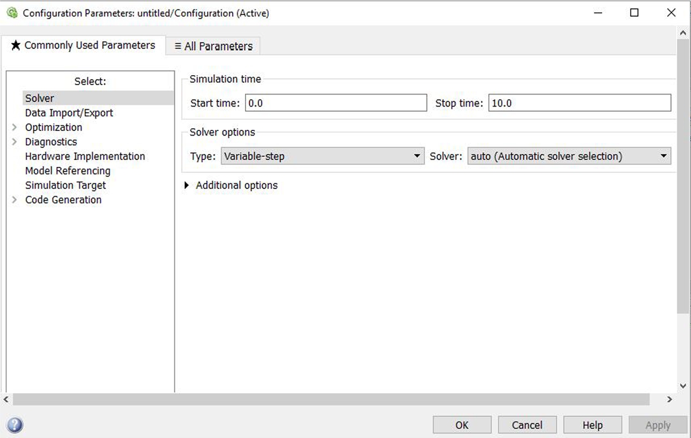
FIGURE 16.5 Simulink window illustrating the solver configuration; this is opened by clicking the icon to the right of the Library Browser icon.
Close the model by clicking the x in the upper right-hand corner of the model window. To open this file again double-click on it in the Current Folder window on the MATLAB desktop. We will build a simple model in this file window in the beginning of the next section of this chapter.
It is expected, of course, that the reader reproduce the next example on data analysis and subsequent examples on dynamic-system modeling to study the application of Simulink to solve technical computing problems. The examples are relatively simple; they are similar to the dynamic system problems examined in Chapters 14 and 17 with MATLAB codes.
To illustrate the mechanics of constructing a model let us consider a signal-processing example. In this example we are going to examine the output from a sine-wave generator. We will integrate the area under the sine wave and compare this with the original signal on a scope, a device that plots the sine wave and the integral of the sine wave with respect to time from time equal to zero, i.e., the time the simulation is started, to the specified time (in this case the default is 10). This model was built by applying the following steps.
1. Point-and-click on the “Sources” icon in the Simulink Library Browser. This opens a palette from which we want to drag the “Sine Wave” and drop it onto the Example1 window illustrated in Figure 16.4 (we are trying to construct the model illustrated in Figure 16.6). This sine wave generator is what we need to provide the input to the model we are building in this section.
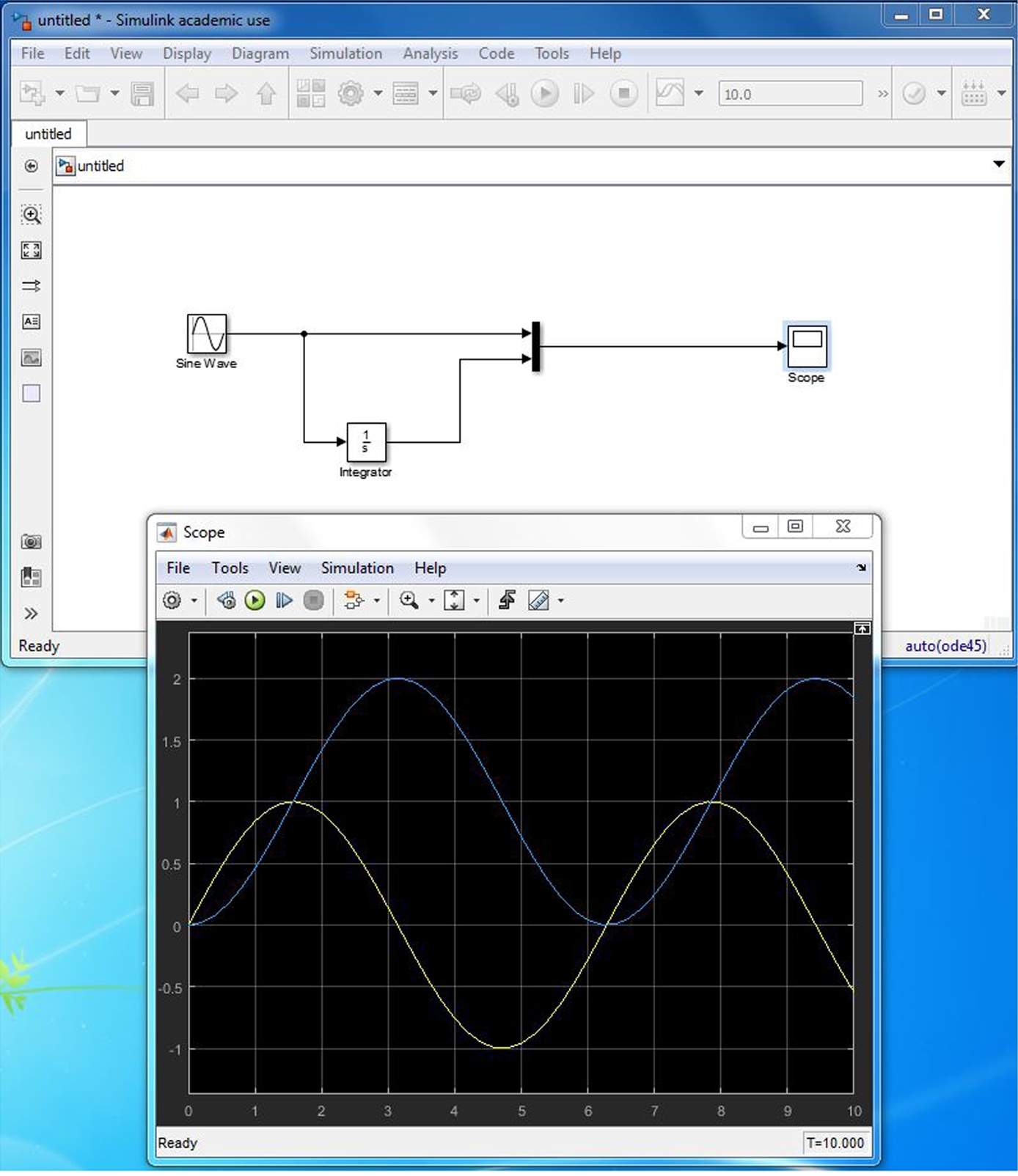
FIGURE 16.6 The Example1 model and the scope illustrating the results of this simulation.
2. Next, open up the “Commonly Used Blocks” by scrolling up the contents and pointing-and-clicking on this topic to open up another palette. Find on this palette a “Scope”, an “Integrator”, and a “Mux”. Next, drag and drop each of these devices onto the Example1 window.
3. In the Example1 window drag the cursor to the right-side output port of the “Sine Wave” generator. When you see the cross, hold the left-mouse button down and drag the cross to the top-left input port of the “Mux”. This is one way to connect a “wire” from one device to the next.
4. Following the same procedure connect the right-side port of the “Mux” to the left-side input port of the “Scope”.
5. Starting at the left-side input port of the “Integrator” hold the left-mouse button down and move to any location on the wire already connecting the “Sine Wave” generator to the “Mux”.
6. Finally, connect the right-side output port of the “Integrator” to the lower-left input port of the “Mux”.
7. Pull down the file menu and click “save” to save your work. In this example we already saved the name of this file, viz., Example1.mdl.
8. To continue, double click on the “Scope” to open the Scope window.
9. Finally, click on the model window to make sure it is in the forefront. To start the simulation hold the keys “Ctrl” and “T” down simultaneously.
You should see two curves appear on the scope. It will be the sine wave (yellow) and the integral of the sine wave (magenta). The “Mux” allows for two inputs into the scope. The model and the results of its execution are illustrated in Figure 16.6.
Of course, if you haven't had any experience with experimental equipment like oscilloscopes, sine-wave generators, multiplexers and the like, much of this may seem a bit mysterious. In addition, the exercise above is only a look-see exercise. It hardly demonstrates the many more powerful features available within Simulink. However, more experience in your technical training and education will allow you to explore more productively this powerful tool and clear up many of these matters. In addition, learning more about Simulink by exercising many of the examples described in the help documentation will help to understand the other toolboxes, e.g., the Control Systems Toolbox. Furthermore, in courses on Dynamical Systems in mechanical and in electrical engineering, many of the available textbooks ask the student to apply Simulink to investigate the systems examined. Thus, there are numerous sources with sample applications, including searching the computer web, that should prove beneficial in learning how to apply this tool to solve more substantial problems in engineering and science. Additional details on the various utilities applied in the above example can be found in the help. We next examine one of the simplest yet quite useful dynamic system.
16.1. Mass-spring-damper dynamic system
The simplest ordinary differential equation that can be used to investigate the oscillation of a dynamic system is the following differential equation:
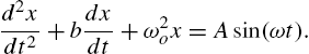 (16.1)
The equation can be used to describe the motion of a mechanical system modeled by a mass, spring and damper forced by a sinusoidal forcing function, where ![]() is the resistance coefficient divided by the mass, m, of a lumped object,
is the resistance coefficient divided by the mass, m, of a lumped object, ![]() is the angular frequency of oscillation of the undamped (
is the angular frequency of oscillation of the undamped (![]() ) motion with a spring-restoration force coefficient k. This is, of course, Newton's second law of motion applied to the forced motion of a dynamic system modeled as a lumped mass acted on by an imposed harmonic force with amplitude
) motion with a spring-restoration force coefficient k. This is, of course, Newton's second law of motion applied to the forced motion of a dynamic system modeled as a lumped mass acted on by an imposed harmonic force with amplitude ![]() , where F is the amplitude of force applied to the system. This is one of the first problems typically investigated in a course on dynamics when examining the oscillatory motion of a particle in one dimension. Let us rewrite this equation as follows:
, where F is the amplitude of force applied to the system. This is one of the first problems typically investigated in a course on dynamics when examining the oscillatory motion of a particle in one dimension. Let us rewrite this equation as follows:
 (16.2)
To solve a differential equation requires integration. Since this is a second order equation we need to integrate twice to obtain a solution. A Simulink model to solve this equation is illustrated in 16.7. Note that the input to “Integrator1” is the sum of the right-hand side of the above equation, i.e., it is the value of the acceleration, ![]() . The output is the speed,
. The output is the speed, ![]() , which is the input to “Integrator2”. Finally, the output of “Integrator2” is the solution at one time step. The details of the simulation illustrated in the figure is described next.
, which is the input to “Integrator2”. Finally, the output of “Integrator2” is the solution at one time step. The details of the simulation illustrated in the figure is described next.
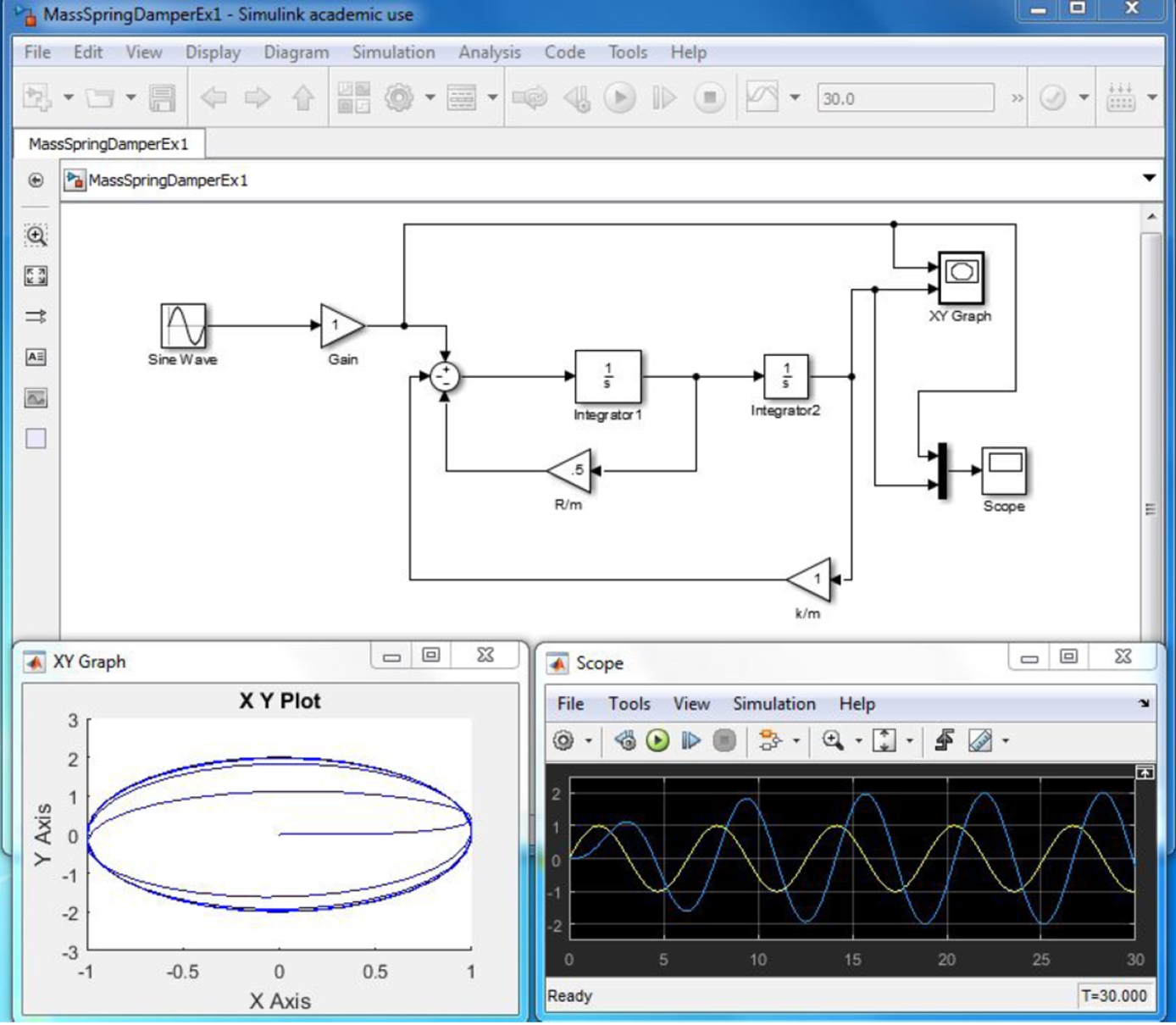
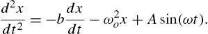
FIGURE 16.7 The MassSpringDamperEx1.mdl model, the X-Y plotter and the scope illustrating the results of this simulation are illustrated in this figure.
The case illustrated is for ![]() and
and ![]() . The initial position x and the initial velocity
. The initial position x and the initial velocity ![]() are equal to zero. In addition, the force on the system at
are equal to zero. In addition, the force on the system at ![]() is zero. The results indicate that for the forcing frequency of
is zero. The results indicate that for the forcing frequency of ![]() radian per unit time and amplitude
radian per unit time and amplitude ![]() , the ultimate amplitude of the motion of the mass is about 2. There is an approximate phase lag of about
, the ultimate amplitude of the motion of the mass is about 2. There is an approximate phase lag of about ![]() between the response and the forcing. Since the forcing frequency is very nearly at the resonance frequency the results illustrated in the figure are consistent with what is reported in the literature, e.g., in Becker (1953).1 As an exercise vary the forcing frequency by double clicking on the “Sine Wave” generator and change the number just below “Frequency (rad/sec):”. Try, e.g., frequencies in the range
between the response and the forcing. Since the forcing frequency is very nearly at the resonance frequency the results illustrated in the figure are consistent with what is reported in the literature, e.g., in Becker (1953).1 As an exercise vary the forcing frequency by double clicking on the “Sine Wave” generator and change the number just below “Frequency (rad/sec):”. Try, e.g., frequencies in the range ![]() and compare your results with the example just described. Find a text on mechanics (or dynamics) to compare your results from Simulink with the theoretical results on this problem reported in the literature.
and compare your results with the example just described. Find a text on mechanics (or dynamics) to compare your results from Simulink with the theoretical results on this problem reported in the literature.
16.2. Bouncing ball dynamic system
This section illustrates the application of initial conditions other than zero (as in the previous section). The model is a modification of the bouncing ball model by MathWorks (Copyright 1990–2010 The MathWorks, Inc.) described in the help; it can be found by typing “Simulation of a bouncing ball” into the search space just below the far left of the tool bar in the “? help” window. The help window can be opened by clicking the circled question mark in the upper tool bar on the MATLAB desktop. Figure 16.8 illustrates the application of initial conditions to the integrals.
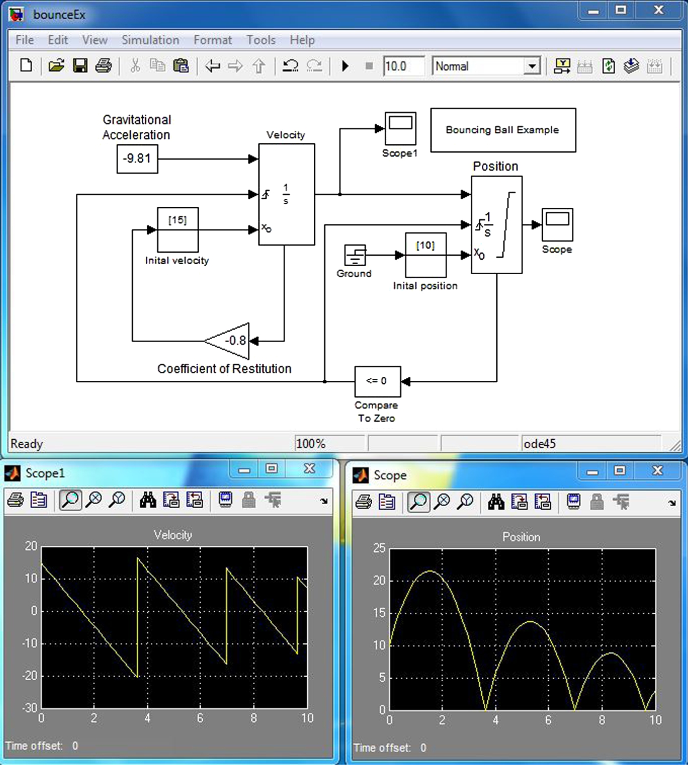
FIGURE 16.8 The bouncing ball model: The velocity and position of the ball are illustrated on the scopes.
This bouncing-ball model is an example of a hybrid dynamic system. A hybrid dynamic system is a system that involves both continuous dynamics, as well as, discrete transitions where the system dynamics can change and the state values can jump. The continuous dynamics of a bouncing ball is simply given by the following equation
 (16.3)
where g is the acceleration due to gravity, x is the vertical distance of the ball after it is released from a specified height, ![]() at a specified speed,
at a specified speed, ![]() . The ground is assumed to be at
. The ground is assumed to be at ![]() . Therefore, the system has two continuous states: position, x, and velocity,
. Therefore, the system has two continuous states: position, x, and velocity, ![]() .
.
The hybrid system aspect of the model originates from the modeling of a collision of the ball with the ground. If one assumes a partially elastic collision with the ground, then the velocity before the collision, ![]() , and velocity after the collision,
, and velocity after the collision, ![]() , can be related by the coefficient of restitution of the ball, κ, as follows:
, can be related by the coefficient of restitution of the ball, κ, as follows:
![]()
The bouncing ball therefore displays a jump in a continuous state (velocity) at the transition condition, ![]() . This discussion is a paraphrase of the information on this problem given in the electronically available help files that come with MATLAB.
. This discussion is a paraphrase of the information on this problem given in the electronically available help files that come with MATLAB.
Let us examine the application of the integrators in this example. The first integrator is labeled “Velocity”. Double clicking on top of this icon with the left mouse opens a window that gives the integrator parameters that are set for this form of the integrator. The external reset is set to “rising”. The initial condition source is set to “external”. The “Show state port” and “Enable zero-crossing detection” are the only items checked. This is illustrated in Figure 16.9. The integrator parameters for the integrator labeled “Position” is shown in Figure 16.10. The top left input port of the two integrators is the input. The bottom two ports allow the initial condition to change at particular intervals of time; in this example, the time to change is associated with the time at which the ball hits the ground. More details on the integrator options at your disposal is described in the help. Search for integrator within the help. As pointed out in the help, “the integrator block outputs the integral of its input at the current time step”. Reading the help files and applying the various options will help you learn more about the capabilities of the Simulink utilities. Certainly there are many ways to construct models to solve a particular problem; it depends on the number of utilities that you are familiar. Even with just the few utilities applied in this and in the previous examples, a number of more complex problems can be solved. This is illustrated in the next two examples on nonlinear dynamical systems.
FIGURE 16.9 The bouncing ball model: The velocity and position of the ball are illustrated on the scopes.
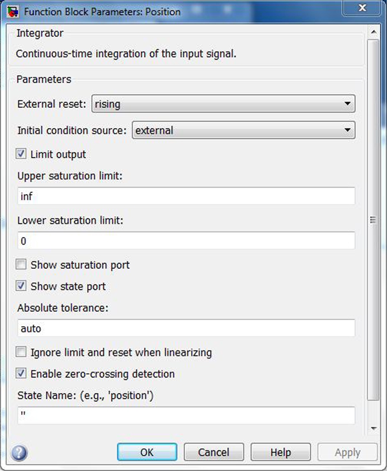
FIGURE 16.10 The bouncing ball model: The velocity and position of the ball are illustrated on the scopes.
16.3. The van der Pol oscillator
In this section we illustrate a model to solve the differential equation known as the van der Pol oscillator. In investigations of nonlinear differential equations and in the study of nonlinear dynamics this equation is one of the first models typically investigated. It has been used, e.g., in the analysis of a vacuum-tube circuit among other practical problems in engineering. The van der Pol equation is
 (16.4)
The interesting thing about finding equations like this one in the engineering and scientific literature is that we can investigate its behavior by applying the technical computing capabilities in MATLAB/Simulink. In this chapter we examine the application of Simulink to solve this equation.2
A Simulink model of this equation is illustrated in Figure 16.11. In this example we selected ![]() . Also, we had to change the initial condition for the device named “Integrator”. The default initial condition of an “Integrator” is zero. To change it you need to double click on the icon and change the initial condition. In this example the initial condition in the second integrator with name “Integrator” was changed to 1. If it is zero, the solution for all time is zero. Applying an initial condition like this one moves the solution from the origin and closer to the limit cycle solution illustrated in the figure. The limit cycle is a single closed curve in the “
. Also, we had to change the initial condition for the device named “Integrator”. The default initial condition of an “Integrator” is zero. To change it you need to double click on the icon and change the initial condition. In this example the initial condition in the second integrator with name “Integrator” was changed to 1. If it is zero, the solution for all time is zero. Applying an initial condition like this one moves the solution from the origin and closer to the limit cycle solution illustrated in the figure. The limit cycle is a single closed curve in the “![]() Graph” that the system approaches for large times away from the initial condition. At time far from the initial condition the system, in this case, reaches a periodic state.
Graph” that the system approaches for large times away from the initial condition. At time far from the initial condition the system, in this case, reaches a periodic state.
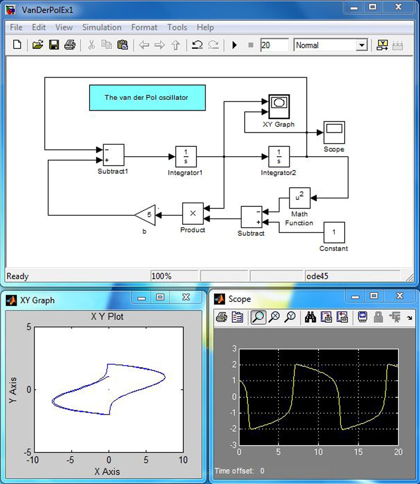
FIGURE 16.11 The van der Pol oscillator: The “Scope” illustrates the solution or output of the oscillator. The “X-Y Graph” is a plot of X = dx/dt versus Y = x.
16.4. The Duffing oscillator
Figure 16.12 illustrates the simulation of a forced nonlinear oscillator modeled by Duffing's equation, viz.,
 (16.5)
This is one of the now classical equations investigated in courses on nonlinear dynamics. In the example illustrated in the figure, ![]() ,
, ![]() ,
, ![]() and
and ![]() . The forcing frequency is
. The forcing frequency is ![]() rad/s. The latter can be verified by double clicking on the “Sine Wave” icon; this operation opens a panel with information about the output of the sine wave generator. For this set of constants the phase portrait, the
rad/s. The latter can be verified by double clicking on the “Sine Wave” icon; this operation opens a panel with information about the output of the sine wave generator. For this set of constants the phase portrait, the ![]() graph in the figure, evolves into a limit cycle or periodic orbit called a “stable period 3 orbit” as described in detail in the book by Guckenheimer and Holmes.3 This example, like the others presented in this chapter, are intended to illustrate that you can study the properties of the solutions to differential equations numerically relatively easily by applying the tools in Simulink (and in MATLAB).
graph in the figure, evolves into a limit cycle or periodic orbit called a “stable period 3 orbit” as described in detail in the book by Guckenheimer and Holmes.3 This example, like the others presented in this chapter, are intended to illustrate that you can study the properties of the solutions to differential equations numerically relatively easily by applying the tools in Simulink (and in MATLAB).
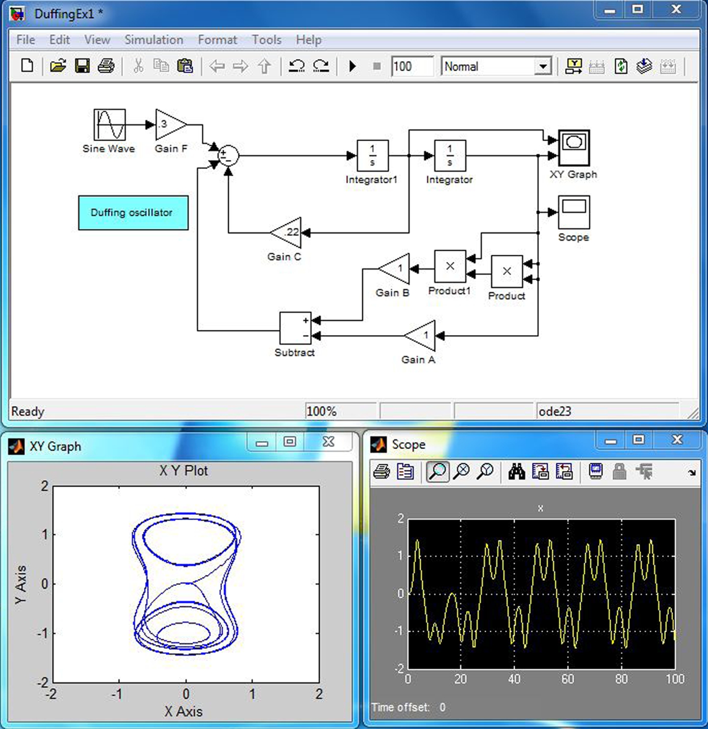
FIGURE 16.12 Forced nonlinear oscillator: The “Scope” compares input forcing (yellow) and output displacement (magenta). The “X-Y Graph” is a plot of X = dx/dt versus Y = x.
There is a wealth of literature on the theory and the numerics of nonlinear equations and, in particular, the Duffing and the van der Pol equations. The theoretical results reported in Guckenheimer and Holmes helped the author select the constants applied in this example. Suggestions for changes in the constants are to be examined in the exercises at the end of this chapter.
Exercises
16.1 Reproduce the signal processing model, i.e., first example in this chapter on the display of the sine and its integral. Execute the simulation to make sure it works (i.e., compares favorably with the results in the example). Next, do the following:
(a) Double click on the integrator and change the initial condition from 0 to 1. Apply the change by clicking the button in the lower right corner of the integrator function block. Execute the simulation. What is the maximum value of the integral? What is the minimum value of the integral?
(b) Double click on the sine wave icon and change the frequency from 1 to 2 and the amplitude from 1 to 2. Apply the changes by clicking the button in the lower right corner of the sine wave source block. Execute the simulation. Note that the frequency is doubled and the amplitude is doubled.
(c) Change the phase of the sine wave from 0 to ![]() . Make sure that the amplitude and frequency are set equal to 1. Apply the changes and execute the simulation. Note that the input function is a cosine instead of a sine function.
. Make sure that the amplitude and frequency are set equal to 1. Apply the changes and execute the simulation. Note that the input function is a cosine instead of a sine function.
16.2 Reproduce the bouncing-ball model and execute it to determine that your reproduction is consistent with the example in this chapter. With a working code examine changes in the coefficient of restitution. Consider several values in the range ![]() . Also examine changes in the initial conditions for
. Also examine changes in the initial conditions for ![]() . To change the value of κ you need to double click on the icon for the coefficient of restitution, change its value and apply it. The same is done to change the initial velocity or the initial position. Once you examine a few different cases explain what you found.
. To change the value of κ you need to double click on the icon for the coefficient of restitution, change its value and apply it. The same is done to change the initial velocity or the initial position. Once you examine a few different cases explain what you found.
16.3 Reproduce the model for a forced spring-mass-damper mechanical system. Remove the “![]() Graph”, its connecting wires, the “Mux” and its connecting wires. Then reattach the “Scope” to the wire attached to the output of “Integrator2”. The model is the spring-mass-damper model with a step change in the force applied at
Graph”, its connecting wires, the “Mux” and its connecting wires. Then reattach the “Scope” to the wire attached to the output of “Integrator2”. The model is the spring-mass-damper model with a step change in the force applied at ![]() as can be verified by double clicking on the “Step” icon; change the “Step time” from the default value of 1 to zero if the time the step is applied is not equal to zero. Set the resistance coefficient
as can be verified by double clicking on the “Step” icon; change the “Step time” from the default value of 1 to zero if the time the step is applied is not equal to zero. Set the resistance coefficient ![]() to zero. Leave
to zero. Leave ![]() , i.e., the spring constant coefficient. Execute the simulation. What is the frequency of oscillation? Examine
, i.e., the spring constant coefficient. Execute the simulation. What is the frequency of oscillation? Examine ![]() , 1, 2 and 4 to determine the effect of increased damping on the solution. If you look this problem up in a physics book on mechanics it is usually under the topic “damped harmonic oscillator”. If
, 1, 2 and 4 to determine the effect of increased damping on the solution. If you look this problem up in a physics book on mechanics it is usually under the topic “damped harmonic oscillator”. If ![]() , it is the harmonic oscillator solution known as simple-harmonic motion; this should have been the solution that you found as part of the examination of the dynamic system in this problem. Without damping (i.e.,
, it is the harmonic oscillator solution known as simple-harmonic motion; this should have been the solution that you found as part of the examination of the dynamic system in this problem. Without damping (i.e., ![]() ) the solution is a sinusoidal motion with constant amplitude. The frequency of oscillation is the natural frequency,
) the solution is a sinusoidal motion with constant amplitude. The frequency of oscillation is the natural frequency, ![]() in this case. Thus, it is not unexpected that a cycle of oscillation occurs over a time interval of 2π; review your results to make sure that this is the case. If
in this case. Thus, it is not unexpected that a cycle of oscillation occurs over a time interval of 2π; review your results to make sure that this is the case. If ![]() , then the motion is critically damped. This means that the dynamic system reaches its infinite time, constant valued solution without overshoot. If
, then the motion is critically damped. This means that the dynamic system reaches its infinite time, constant valued solution without overshoot. If ![]() is less than this value, the system is said to be underdamped. If
is less than this value, the system is said to be underdamped. If ![]() is greater than this value, the system is said to be overdamped. Setting
is greater than this value, the system is said to be overdamped. Setting ![]() leads to a critically damped behavior. Describe, from your solutions for the range of
leads to a critically damped behavior. Describe, from your solutions for the range of ![]() considered in this problem, the meaning of underdamped, critically damped and overdamped response (as reflected in the solution x) of the system for the mechanical system examined in this problem.
considered in this problem, the meaning of underdamped, critically damped and overdamped response (as reflected in the solution x) of the system for the mechanical system examined in this problem.
16.4 In the previous problem try the damping coefficient ![]() . Describe the results. Notice how the amplitude grows with time. Thus, with a negative resistance coefficient we have growth in the amplitude of the solution. If you set
. Describe the results. Notice how the amplitude grows with time. Thus, with a negative resistance coefficient we have growth in the amplitude of the solution. If you set ![]() , you can investigate exponential growth. Create a problem that you provide a solution that deals with the problem of exponential growth.
, you can investigate exponential growth. Create a problem that you provide a solution that deals with the problem of exponential growth.
16.5 Reproduce the van der Pol oscillator model. Execute the simulation to compare your results with the results in the example (this is, of course, a necessary step to check your computer code). Next, set the damping coefficient ![]() . Execute the simulation. The result should be simple-harmonic motion of amplitude unity because the initial condition in the second integrator was set equal to unity and period equal to 2π. Next, examine the case for
. Execute the simulation. The result should be simple-harmonic motion of amplitude unity because the initial condition in the second integrator was set equal to unity and period equal to 2π. Next, examine the case for ![]() . Finally, examine
. Finally, examine ![]() . Note the qualitative changes in the response function, i.e., in the plotted values of x.
. Note the qualitative changes in the response function, i.e., in the plotted values of x.
16.6 Reproduce the Duffing oscillator model. Execute the simulation to compare your results with the results in the example. Set the parameters ![]() . The result is forced harmonic motion at a single frequency. Try examining the linear case, which means
. The result is forced harmonic motion at a single frequency. Try examining the linear case, which means ![]() , and
, and ![]() , which means a spring. In all cases the motion ends up being a forced harmonic motion of a single sinusoidal frequency. This is because the cubic-nonlinear term was suppressed by setting
, which means a spring. In all cases the motion ends up being a forced harmonic motion of a single sinusoidal frequency. This is because the cubic-nonlinear term was suppressed by setting ![]() . (There are many other combinations that you can explore. However, be aware of the fact that some combinations of parameters lead to chaotic solutions and, hence, may never settle down to a periodic state. There also may be parameter selections that lead to unstable solutions.)
. (There are many other combinations that you can explore. However, be aware of the fact that some combinations of parameters lead to chaotic solutions and, hence, may never settle down to a periodic state. There also may be parameter selections that lead to unstable solutions.)
Appendix 16.A. Supplementary material
Supplementary material related to this chapter can be found online at http://dx.doi.org/10.1016/B978-0-08-100877-5.00018-9.
1 “Becker, R.A. (1953): Introduction to Theoretical Mechanics, McGraw-Hill Book Company, NY.”
2 “More can be found by searching in the help by clicking the question mark and searching for “van der Pol”. A Simulink demo is one of the items that comes up when the search term used is as quoted.”
3 “Guckenheimer, John, & Philip Holmes (1983): Nonlinear Oscillations, Dynamical Systems, and Bifurcations of Vector Fields, Springer-Verlag, NY.”