Plan, Activity, and Intent Recognition: Theory and Practice, FIRST EDITION (2014)
Part II. Activity Discovery and Recognition
Chapter 5. Stream Sequence Mining for Human Activity Discovery
Parisa Rashidi, University of Florida, Gainesville, FL, USA
Abstract
During the past decade, supervised activity recognition methods have been studied by many researchers; however, these methods still face many challenges in real-world settings. Supervised activity recognition methods assume that we are provided with labeled training examples from a set of predefined activities. Annotating and hand-labeling data is a very time-consuming and laborious task. Also, the assumption of consistent predefined activities might not hold in reality. More important, these algorithms do not take into account the streaming nature of data, or the possibility that the patterns might change over time. This chapter provides an overview of the state-of-the-art unsupervisedmethods for activity recognition. In particular, we describe a scalable activity discovery and recognition method for complex large real-world datasets based on sequential data mining and stream data mining methods.
Keywords
activity discovery
activity recognition
unsupervised learning
sequence mining
stream mining
5.1 Introduction
Remarkable recent advancements in sensor technology and sensor networking are leading us into a world of ubiquitous computing. Many researchers are now working on smart environments that can respond to the needs of the residents in a context-aware manner by using sensor technology. Along with data mining and machine learning techniques [12]. For example, smart homes have proven to be of great value for monitoring physical and cognitive health through analysis of daily activities [54]. Besides health monitoring and assisted living, smart homes can be quite useful for providing more comfort, security, and automation for the residents. Some of the efforts for realizing the vision of smart homes have been demonstrated in the real-world testbeds such as CASAS [51], MavHome [14], DOMUS [7], iDorm [17], House_n [61], and Aware Home [1].
A smart environment typically contains many highly interactive devices, as well as different types of sensors. The data collected from these sensors is used by various data mining and machine learning techniques to discover residents’ activity patterns and then to recognize such patterns later [28,31]. Recognizing activities allows the smart environment to respond in a context-aware way to the residents’ needs [21,50,70,67].
Activity recognition is one of the most important components of many pervasive computing systems. Here, we define an activity as a sequence of steps performed by a human actor to achieve a certain goal. Each step should be measurable by a sensor state or a combination of sensor states. It should be noted that besides activities, we can recognize other types of concepts such as situations or goals. We define a situation as a snapshot of states at a specific time point in a physical or conceptual environment.
Unlike activities, situations try to model high-level interpretation of phenomena in an environment. An example of an activity would be pouring hot water into a cup, but making tea would constitute a situation, according to these definitions. Rather than trying to figure out the purpose of a user from sensor data, it is also possible to define goals for users (e.g., each goal is the objective realized by performing an activity). The boundaries between those concepts are often blurred in practice. This chapter focuses on the problem of activity recognition.
Data in a smart home are collected from different types of ambient sensors. For example, a Passive Infrared Sensor (PIR) can be used for detecting motion, and a contact switch sensor can be used for detecting the open/close status of doors and cabinets. Some of the most widely used smart home sensors are summarized in Table 5.1. Most of the ambient sensors, such as the PIR sensor or the contact switch sensor, provide a signal in the form of on/off activation states, as depicted in Figure 5.1.
Table 5.1
Ambient Sensors Used in Smart Environments
|
Sensor |
Measurement |
Data format |
|
PIRa |
Motion |
Categorical |
|
Active infrared |
Motion/identification |
Categorical |
|
RFIDb |
Object information |
Categorical |
|
Pressure |
Surface pressure |
Numeric |
|
Smart tile |
Floor pressure |
Numeric |
|
Magnetic switch |
Open/close |
Categorical |
|
Ultrasonic |
Motion |
Numeric |
|
Camera |
Activity |
Image |
|
Microphone |
Activity |
Sound |
a Passive Infrared Motion Sensor
b Radio Frequency Identification
Note: The PIR sensor is one of the most popular sensors used by many researchers for detecting motion. Other options, such as ultrasonic sensors, might prove more accurate for detecting motion; however, they are typically more expensive.
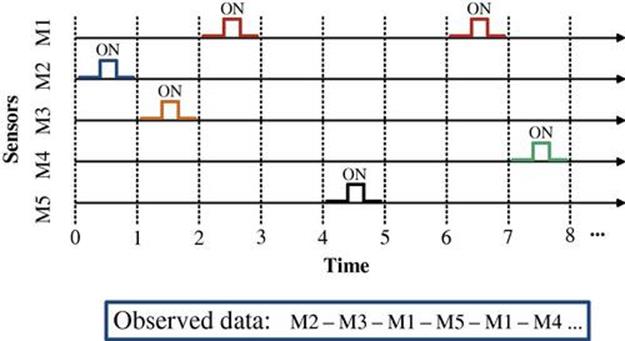
FIGURE 5.1 A stream of sensor events. Note: Each one of the M1 through M5 symbols correspond to one sensor. For example, sensor M1 is activated during the third and seventh time intervals, and M5 is activated during the fifth time interval.
Before using sensor data in machine learning and data mining tasks, data are usually preprocessed into a higher-level format that is easier to interpret. For example, the signal levels are converted into categorical values, such as on/off binary values, in the case of PIR sensors. Table 5.2 shows an example format typically used in data mining and machine learning tasks.1
Table 5.2
Example Sensor Data
|
Timestamp |
Sensor ID |
Label |
|
7/17/2009 09:52:25 |
M3 |
Personal Hygiene |
|
7/17/2009 09:56:55 |
M5 |
Personal Hygiene |
|
7/17/2009 14:12:20 |
M4 |
None |
As soon as data are collected from various sensors, they are passed to an activity recognition component. In supervised activity recognition methods, the algorithm is provided with the activity label of sensor event sequences. These labels are hand-done by a human annotator during the training phase of the system. Some researchers also have taken advantage of the crowdsourcing mechanism for labeling [72,59]. In Table 5.2, the first and the second sensor events are labeled Personal Hygiene activity. The ultimate goal is to predict the label of the future unseen activity patterns by generalizing based on the examples provided.
During the past decade, many supervised activity recognition algorithms have been proposed [8,61,65,13,31,47,57,39]. In real-world settings, using supervised methods is not practical because it requires labeled data for training. Manual labeling of human activity data is time consuming, laborious, and error-prone. Besides, one usually needs to deploy invasive devices in the environment during the data-collection phase to obtain reliable annotations. Another option is to ask the residents to report their activities. Asking residents to report their activities puts the burden on them, and in the case of the elderly with memory problems (e.g., dementia), it would be out the of question.
To address the annotation problem, recently a few unsupervised methods have been proposed for mining human activity data [23,44,51,58,54]. However, none of these mining approaches take into account the streaming nature of data or the possibility that patterns might change over time. In a real-world smart environment, we have to deal with a potentially infinite and unbounded flow of data. In addition, the discovered activity patterns can change from time to time. Mining the stream of data over time not only allows us to find new emerging patterns in the data, but it also allows us to detect changes in the patterns, which can be beneficial for many applications. For example, a caregiver can look at the pattern trends and spot any suspicious changes immediately.
Based on these insights, we extend a well-known stream mining method [20] in order to discover activity pattern sequences over time. Our activity discovery method allows us to find discontinuous varied-order patterns in streaming, nontransactional sensor data over time. The details of the model will be discussed in Section 5.3.2
5.2 Related Work
The following subsections provide a literature overview of several subjects. First we discuss the general activity recognition problem. Then, we describe various sequence mining and stream mining methods. Finally, we review activity discovery methods based on data mining approaches in more detail.
5.2.1 Activity Recognition
In recent years, many approaches have been proposed for activity recognition in different settings such as methods for recognizing nurses’ activities in hospitals [57], recognizing quality inspection activities during car production [41], monitoring elderly adults’ activities [13], studying athletic performance [4,40], gait analysis in diseases (e.g., Parkinson’s [56,45,33], emergency response [34], and monitoring unattended patients [15]. Activity discovery and recognition approaches not only differ according to the deployed environment but also with respect to the type of activity data collected, the model used for learning the activity patterns, and the method used for annotating the sample data. The following subsections explain each aspect in more detail.
5.2.1.1 Activity data
Activity data in smart environments can be captured using different media depending on the target environment and also target activities. Activity data at home can be collected with ambient sensors (e.g., infrared motion) to track the motion of residents around home [51]. Additional ambient sensors, such as temperature sensors, pressure sensors, contact switch sensors, water sensors, and smart power-meters, can provide other types of context information. For recognizing residents’ interaction with key objects, some researchers have used object sensors (e.g., RFID tags) that can be placed on key items [61,47].
Another type of sensor used for recognizing activities are wearable sensors such as accelerometers [39,69]. More recent research uses mobile phones as carryable sensors [74]. The advantage of wearable and mobile sensors is their ability to capture activity data in both indoor and outdoor settings. Their main disadvantage is their obtrusiveness because the user is required to carry the sensor all the time.
Besides ambient sensors and wearable sensors, surveillance cameras and other types of image-capturing devices (e.g., thermographic cameras) have been used for activity recognition [60]. However, individuals are usually reluctant to use cameras for capturing activity data due to privacy concerns [29]. Another limitation for using cameras is that activity recognition methods based on video-processing techniques can be computationally expensive.
5.2.1.2 Activity models
The number of machine learning models that have been used for activity recognition varies almost as widely as the types of sensor data that have been obtained. Naive Bayes classifiers have been used with promising results for activity recognition [8,61,65]. Other methods, such as decision trees, Markov models, dynamic Bayes networks, and conditional random fields, have also been successfully employed [13,31,47,57,39]. There also have been a number of works in the activity discovery area using unsupervised methods—to be discussed in Section 5.2.4.
5.2.1.3 Activity annotation
Another aspect of activity recognition is the method for annotating the sample training data. Most of the researchers have published results of experiments in which the participants are required to manually note each activity they perform at the time they perform it [31,61,47]. In other cases, the experimenters told the participants which specific activities should be performed, so the correct activity labels were identified before sensor data were even collected [13,23,39]. In some cases, the experimenter manually inspects the raw sensor data in order to annotate it with a corresponding activity label [67]. Researchers have also used methods, such as experience sampling [61], where subjects carry a mobile device to use for self-reporting.
5.2.2 Sequence Mining
Sequence mining has already proven to be quite beneficial in many domains such as marketing analysis or Web click-stream analysis [19]. A sequence ![]() is defined as a set of ordered items denoted by
is defined as a set of ordered items denoted by ![]() . In activity recognition problems, the sequence is typically ordered using timestamps. The goal of sequence mining is to discover interesting patterns in data with respect to some subjective or objective measure of how interesting it is. Typically, this task involves discovering frequent sequential patterns with respect to a frequency support measure.
. In activity recognition problems, the sequence is typically ordered using timestamps. The goal of sequence mining is to discover interesting patterns in data with respect to some subjective or objective measure of how interesting it is. Typically, this task involves discovering frequent sequential patterns with respect to a frequency support measure.
The task of discovering all the frequent sequences is not a trivial one. In fact, it can be quite challenging due to the combinatorial and exponential search space [19]. Over the past decade, a number of sequence mining methods have been proposed that handle the exponential search by using various heuristics. The first sequence mining algorithm was called GSP [3], which was based on the a priori approach for mining frequent itemsets [2]. GSP makes several passes over the database to count the support of each sequence and to generate candidates. Then, it prunes the sequences with a support count below the minimum support.
Many other algorithms have been proposed to extend the GSP algorithm. One example is the PSP algorithm, which uses a prefix-based tree to represent candidate patterns [38]. FREESPAN [26] and PREFIXSPAN [43] are among the first algorithms to consider a projection method for mining sequential patterns, by recursively projecting sequence databases into smaller projected databases. SPADE is another algorithm that needs only three passes over the database to discover sequential patterns [71]. SPAM was the first algorithm to use a vertical bitmap representation of a database [5]. Some other algorithms focus on discovering specific types of frequent patterns. For example, BIDE is an efficient algorithm for mining frequent closed sequences without candidate maintenance [66]; there are also methods for constraint-based sequential pattern mining [44].
5.2.3 Stream Mining
Compared to the classic problem of mining sequential patterns from a static database, mining sequential patterns over datastreams is far more challenging. In a datastream, new elements are generated continuously and no blocking operation can be performed on the data. Despite such challenges, with the rapid emergence of new application domains over the past few years, the stream mining problem has been studied in a wide range of application domains. A few such application domains include network traffic analysis, fraud detection, Web click-stream mining, power consumption measurements, and trend learning [11,19].
For finding patterns in a datastream, using approximation based on a relaxed support threshold is a key concept [9,36]. The first stream mining approach was based on using a landmark model and calculating the count of the patterns from the start of the stream[36]. Later, methods were proposed for incorporating the discovered patterns into a prefix tree [18]. More recent approaches have introduced methods for managing the history of items over time [20,62]. The main idea is that one usually is more interested in details of recent changes, while older changes are preferred in coarser granularity over the long term.
The preceding methods discover frequent itemsets in streaming data. There are also several other methods for finding sequential patterns over datastreams, including the SPEED algorithm [49], approximate sequential pattern mining in Web usage [37], a data cubing algorithm [25], and mining multidimensional sequential patterns over datastreams [48].
All of the sequential stream mining approaches consider data to be in a transactional format. However, the input datastream in a smart environment is a continuous flow of unbounded data. The sensor data has no boundaries separating different activities or episodes from each other, and it is just a continuous stream of sensor events over time. Figure 5.2 depicts the difference between transaction data and sensor data. As can be seen in Figure 5.2(a), in transaction data, each single transaction is associated with a set of items and is identified by a transaction ID, making it clearly separated from the next transaction. The sensor data has no boundaries separating different activities or episodes from each other, and it is just a continuous stream of sensor events over time. This property makes it a unique, challenging stream mining problem. To deal with this, we use a compression-based approach to group together the cooccurring events into varied-order discontinuous activity patterns. The details will be explained in Section 5.3.
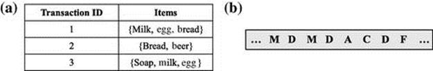
FIGURE 5.2 Boundary problem in transaction data versus sensor data. Each symbol in (b) corresponds to one sensor event, and a sequence of such sensor events might represent an activity. However, it would be difficult to estimate the boundaries of activities. (a) In transaction data, there is a clear boundary between consecutive transactions; (b) The sensor data have no boundaries separating different activities or episodes from each other.
5.2.4 Data Mining for Activity Discovery
Unlike supervised methods, unsupervised methods do not require any labeled sensor data. Instead, they try to automatically find interesting activity patterns in unlabeled sensor data. A number of different unsupervised approaches have been proposed in the past for discovering activity patterns.
One popular approach is to extend current data mining techniques in the context of activity recognition tasks. These methods look for regularly occurring interactions, and discover significant patterns with respect to measures such as frequency or periodicity. For example, Heierman et al. [28] discovered subsequences, or episodes, that are closely related in time. These episodes may be partially ordered and are evaluated based on information theory principles.
Gu et al. [23] use a frequency measure to discover emerging patterns and use feature relevance to segment the boundary of any two adjacent activities. More recently, they have extended their model to recognize sequential, interleaved, and concurrent activities using changes between classes of data [22]. Previously, we also have proposed a method for simultaneous discovery of frequent and periodic patterns using the minimum description length principle [51].
Another approach to activity discovery relies on time series techniques, especially in the context of activity data collected from wearable sensors such as accelerometers. For example, Vahdatpour et al. [64] analyze multidimensional time series data by locating multidimensional motifs in time series. Similarly Zhao [73] converts times series activity data into a set of motifs for each data dimension, where each motif represents an approximately repeated symbolic subsequence. These motifs serve as the basis for a large candidate set of features, which later is used for training a conditional random field model.
The problem of unsupervised activity recognition also has been explored using vision community to discover activities from a set of images or from videos. For example, Mahajan et al. [35] used a finite state machine network in an unsupervised mode that learns the usual patterns of activities in a scene over long periods of time. During the recognition phase, the usual activities are accepted as normal, and deviant activity patterns are flagged as abnormal.
Other unsupervised options for activity discovery include techniques such as mixture models and dimensionality reduction. Schiele et al. [58] detect activity structure using low-dimensional Eigenspaces, and Barger et al. [6] use mixture models to develop a probabilistic model of behavioral patterns. Huynh et al. [30] also use a combination of discriminative and generative methods to achieve reduced supervision for activity recognition. As described in another chapter in this book, Nguyen et al. [63] use hierarchical Dirichlet processes (HDP) as a Bayesian nonparametric method to infer atomic activity patterns without predefining the number of latent patterns. Their work focuses on using a nonparametric method to infer the latent patterns, while we explore the problem of inferring discontinuous and dynamic patterns from a datastream.
It is also possible to combine background knowledge with unsupervised activity discovery methods to aid the discovery process. For example, Dimitrov et al. [16] use background domain knowledge about user activities and the environment in combination with probabilistic reasoning methods to build a possible explanation of the observed stream of sensor events. Also, a number of methods mine activity definitions from the Web by treating it as a large repository of background knowledge.
Perkowitz et al. [46] mine definitions of activities in an unsupervised manner from the Web. Similarly, Wyatt et al. [68] view activity data as a set of natural language terms. Activity models are considered as mappings from such terms to activity names and are extracted from text corpora (e.g., the Web). Palmes et al. [42] also mine the Web to extract the most relevant objects according to their normalized usage frequency. They develop an algorithm for activity recognition and two algorithms for activity segmentation with linear time complexities.
Unfortunately, none of these activity discovery methods address the problem of streaming data, nor the fact that the patterns might change over time. We explain in Section 5.3 how such challenges can be addressed.
5.3 Proposed Model
Due to the special requirements of our application domain, we cannot directly use the tilted-time window model [20]. First of all, the tilted-time approach, as well as most other similar stream mining methods, was designed to find sequences or itemsets in transaction-based streams [10,37,49]. The data obtained in a smart environment are a continuous stream of unbounded sensor events with no boundary between episodes or activities (refer to Figure 5.2). Second, as discussed in [54], because of the complex and erratic nature of human activity, we need to consider an activity pattern as a sequence of events. In such a sequence, the patterns might be interrupted by irrelevant events (called a discontinuous pattern). Also the order of events in the sequence might change from occurrence to occurrence (called a varied-order pattern).
Finding variations of a general pattern and determining their relative importance can be beneficial in many applications. For example, a study by Hayes et al. found that variation in the overall activity performance at home was correlated with mild cognitive impairment [27]. This highlights the fact that it is important to recognize and monitor all activities and the variations that occur regularly in an individual’s daily environment.
Third, we also need to address the problem of varying frequencies for activities performed in different regions of a home. A person might spend the majority of his or her time in the living room during the day and only go to the bedroom for sleeping. We still need to discover the sleep pattern though its sensor support count might be substantially less than that found by the sensors in the living room.
Our previously introduced sequence mining methods, DVSM [54] and COM [52], do not take into account the streaming nature of data, nor the possibility that the patterns might change over time. In addition, an activity recognition system based on supervised methods, once trained, will not be able to adapt to any changes in the underlying stream. In a real-world situation, we have to deal with a potentially infinite and unbounded flow of data. The discovered activity patterns can also change over time, and algorithms need to detect and respond to such changes. Figure 5.3 better depicts the comparison of supervised, sequence mining, and stream mining approaches. Note that activity discovery and activityannotation in sequence mining and supervised approaches are one-time events, while in the stream mining approach, the patterns are discovered and updated in a continuous manner.
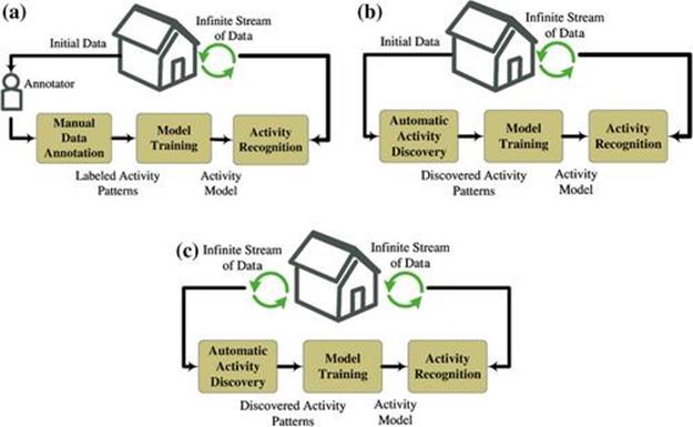
FIGURE 5.3 Comparing different approaches to activity recognition. (a) Supervised; (b) Sequence mining; (c) Stream mining.
To address these issues, we extended the tilted-time window approach [20] to discover activity patterns over time. An extended method, called StreamCOM, allows us to find discontinuous varied-order patterns in streaming sensor data over time. To the best of our knowledge, StreamCOM represents the first reported stream mining method for discovering human activity patterns in sensor data over time [53].
5.3.1 Tilted-Time Window Model
The tilted-time window model allows for managing the history of items over time [20]. It plays an important role in our stream mining model, therefore we explain it in more detail. This approach finds the frequent itemsets using a set of tilted-time windows, such that the frequency of the item is kept at a finer level for recent time frames and at a coarser level for older time frames. Such an approach can be quite useful for human activity pattern discovery. For example, a caregiver is usually interested in the recent changes of the patient at a finer level, and in the older patterns (e.g., from three months ago) at a coarser level.
Figure 5.4 shows an example of a natural tilted-time window, where the frequency of the most recent item is kept with an initial precision granularity of an hour, in another level of granularity in the last 24 h, and then again at another level in the last 30 days. As new data items arrive over time, the history of items will be shifted back in the tilted-time window.
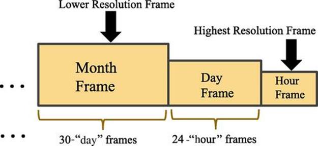
FIGURE 5.4 Natural tilted-time window.
It should be noted that the frequency of a pattern cannot be deterministically determined in the case of streaming data because data is observed only up to a certain point; consequently, the item frequencies reflect the computed frequencies up to that point. This also means that we will have computed frequency (observed frequency computed up to this point) in addition to the actual frequency (which we are unable to observe). Therefore, a pattern that is currently frequent might later become infrequent. Similarly, an infrequent pattern might later turn out to be frequent. Therefore, a relaxed threshold is used to find patterns.
Definition 5.1 Let the minimum support be denoted by ![]() , and the maximum support error be denoted by
, and the maximum support error be denoted by ![]() . An itemset
. An itemset ![]() is said to be frequent if its support is no less than
is said to be frequent if its support is no less than ![]() . If support of
. If support of ![]() is less than
is less than ![]() , but no less than
, but no less than ![]() , it is subfrequent; otherwise, it is considered to be infrequent.
, it is subfrequent; otherwise, it is considered to be infrequent.
The support of an itemset in this definition is defined as the proportion of transactions (events) in the observed dataset that contain the itemset. This definition defines subfrequent patterns (i.e., those patterns of which we are not yet certain about their frequency). Using the approximation approach for frequencies allows for the subfrequent patterns to become frequent later, while discarding infrequent patterns.
To reduce the number of frequency records in the tilted-time windows, the old frequency records of an itemset ![]() are pruned. Let
are pruned. Let ![]() denote the computed frequency of
denote the computed frequency of ![]() in time unit
in time unit ![]() , and let
, and let ![]() denote the number of transactions received within time unit
denote the number of transactions received within time unit ![]() . Also let
. Also let ![]() refer to the most recent time point. For some
refer to the most recent time point. For some ![]() , where
, where ![]() , the frequency records
, the frequency records ![]() are pruned if both Equation 5.1 and Equation 5.2 hold.
are pruned if both Equation 5.1 and Equation 5.2 hold.
![]() (5.1)
(5.1)
 (5.2)
(5.2)
Equation 5.1 finds a point ![]() in the stream such that before that point the computed frequency of the itemset
in the stream such that before that point the computed frequency of the itemset ![]() is always less than the minimum frequency required. Equation 5.2 finds a point
is always less than the minimum frequency required. Equation 5.2 finds a point ![]() , where
, where ![]() , such that before that point the sum of the computed support of
, such that before that point the sum of the computed support of ![]() is always less than the relaxed minimum support threshold. In this case the frequency records of
is always less than the relaxed minimum support threshold. In this case the frequency records of ![]() from
from ![]() to
to ![]() are considered unpromising and are pruned. This type of pruning is referred to as tail pruning [20]. In our model, we extend the preceding defections and pruning techniques for discontinuous, varied order patterns.
are considered unpromising and are pruned. This type of pruning is referred to as tail pruning [20]. In our model, we extend the preceding defections and pruning techniques for discontinuous, varied order patterns.
5.3.2 Tilted-Time Window Model in Current System
The input data in our model are an unbounded stream of sensor events, each in the form of ![]() , where
, where ![]() refers to a sensor ID and
refers to a sensor ID and ![]() refers to the timestamp when sensor
refers to the timestamp when sensor ![]() has been activated. We define an activity instance as a sequence of
has been activated. We define an activity instance as a sequence of ![]() sensor events
sensor events ![]() . Note that in our notation an activity instance is considered as a sequence of sensor events, not a set of unordered events. We are assuming that the sensors capture binary status change events; that is, a sensor can be either on or off.
. Note that in our notation an activity instance is considered as a sequence of sensor events, not a set of unordered events. We are assuming that the sensors capture binary status change events; that is, a sensor can be either on or off.
We assume that the input data are broken into batches ![]() , where each
, where each ![]() is associated with a time period
is associated with a time period ![]() , and the most recent batch is denoted by
, and the most recent batch is denoted by ![]() or for short as
or for short as ![]() . Each batch
. Each batch ![]() contains a number of sensor events, denoted by
contains a number of sensor events, denoted by ![]() .
.
As we mentioned before, we use a tilted-time window for maintaining the history of patterns over time. Instead of maintaining the frequency records, we maintain the compression records, which will be explained in more detail in Section 5.3.3. Also, in our model, as the frequency of an item is not the single deciding factor and other factors (e.g., the length of the pattern and its continuity) also play a role. We use the term interesting pattern instead of frequent pattern.
The original tilted-time model represents data in terms of logarithmic windows [20]. Our tilted-time window is depicted in Figure 5.5. Here, the window keeps the history records of a pattern during the past four weeks at the finer level of week granularity. History records older than four weeks are only kept at the month granularity. In our application domain, we use a different tilted-time window format that is a more natural representation versus a logarithmic tilted-time window. For example, it would be it easier for a nurse or caregiver to interpret the pattern trend using a natural representation. Second, as we don’t expect the activity patterns to change substantially over a very short period of time, we omit the day and hour information for the sake of a more efficient representation. For example, in the case of dementia patients, it takes weeks and/or months to see some changes develop in their daily activity patterns.
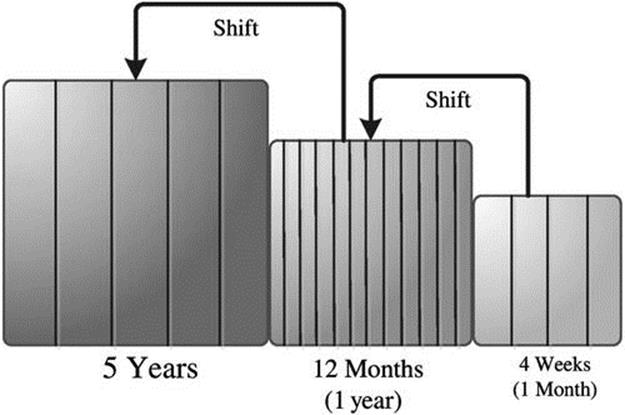
FIGURE 5.5 Our tilted-time window.
Using such a schema, we only need to maintain ![]() compression records instead of
compression records instead of ![]() records in a normal natural tilted-time window. Note that we chose such a representation in this study for the reasons mentioned before. However, if necessary, one can adopt other tilted-window models (e.g., the logarithmic windows) as the choice of tilted-time window has no effect on the model except for efficiency.
records in a normal natural tilted-time window. Note that we chose such a representation in this study for the reasons mentioned before. However, if necessary, one can adopt other tilted-window models (e.g., the logarithmic windows) as the choice of tilted-time window has no effect on the model except for efficiency.
To update the tilted-time window, whenever a new batch of data arrives, we replace the compression values at the finest level of time granularity and shift back to the next level of finest time granularity. During shifting, we check whether the intermediate window is full. If so, the window is shifted back even more; otherwise, the shifting stops.
5.3.3 Mining Activity Patterns
Our goal is to develop a method that can automatically discover resident activity patterns over time from streaming sensor data. This is so even if the patterns are somehow discontinuous or have different event orders across their instances. Both situations happen quite frequently when dealing with human activity data. For example, consider the meal preparation activity. Most people will not perform this activity in exactly the same way each time, rather, some of the steps or the order of the steps might be changed (variations). In addition, the activity might be interrupted by irrelevant events such as answering the phone (discontinuous). Our DVSM and COM methods find such patterns in a static dataset [54]. For example, the pattern ![]() can be discovered from instances
can be discovered from instances ![]() , and
, and ![]() , despite the fact that the events are discontinuous and have varied orders.
, despite the fact that the events are discontinuous and have varied orders.
We discover sequential patterns from current data batch ![]() using an extended version of COM that is able to handle streaming data. After finding patterns in current data batch
using an extended version of COM that is able to handle streaming data. After finding patterns in current data batch ![]() , we update the tilted-time windows and prune any pattern that seems to be unpromising. Figure 5.6 depicts the steps of our activity pattern mining process better.
, we update the tilted-time windows and prune any pattern that seems to be unpromising. Figure 5.6 depicts the steps of our activity pattern mining process better.
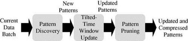
FIGURE 5.6 The activity pattern mining steps.
To find patterns in data, first a reduced batch ![]() is created from the current data batch
is created from the current data batch ![]() . The reduced batch contains only frequent and subfrequent sensor events, which will be used for constructing longer patterns. A minimum support is required to identify such frequent and subfrequent events. COM only identifies the frequent events. Here, we introduce the maximum sensor support error
. The reduced batch contains only frequent and subfrequent sensor events, which will be used for constructing longer patterns. A minimum support is required to identify such frequent and subfrequent events. COM only identifies the frequent events. Here, we introduce the maximum sensor support error ![]() to allow for the subfrequent patterns to be discovered also. In addition, automatically derive multiple minimum support values corresponding to different regions of the space.
to allow for the subfrequent patterns to be discovered also. In addition, automatically derive multiple minimum support values corresponding to different regions of the space.
In mining real-life activity patterns, the frequency of sensor events can vary across different regions of the home or another space. If the differences in sensor event frequencies across different regions of the space are not taken into account, the patterns that occur in less frequently used areas of the space might be ignored. For example, if the resident spends most of his or her time in the living room during the day and only goes to the bedroom for sleeping, then the sensors will be triggered more frequently in the living room than in the bedroom. Therefore, when looking for frequent patterns, the sensor events in the bedroom might be ignored and consequently the sleep pattern might not be discovered. The same problem happens with different types of sensors, as usually the motion sensors are triggered much more frequently than another type of sensor such as cabinet sensors. This problem is known as the rare item problem in market-basket analysis and is usually addressed by providing multiple minimum support values [32].
We automatically derive multiple minimum sensor support values across space and over time. To do this, we identify different regions of the space using location tags ![]() , corresponding to the functional areas such as bedroom, bathroom, and so on. Also different types of sensors might exhibit varying frequencies. In our experiments, we categorized the sensors into motion sensors and interaction-based sensors. The motion sensors are those sensors tracking the motion of a person around a home (e.g., infrared motion sensors). Interaction-based sensors, which we call key sensors, are the non-motion-tracking sensors (e.g., cabinet or RFID tags on items). Based on observing and analyzing sensor frequencies in multiple smart homes, we found that a motion sensor has a higher false positive rate than a key sensor in some other regions. Thus, we derive separate minimum sensor supports for different sensor categories.
, corresponding to the functional areas such as bedroom, bathroom, and so on. Also different types of sensors might exhibit varying frequencies. In our experiments, we categorized the sensors into motion sensors and interaction-based sensors. The motion sensors are those sensors tracking the motion of a person around a home (e.g., infrared motion sensors). Interaction-based sensors, which we call key sensors, are the non-motion-tracking sensors (e.g., cabinet or RFID tags on items). Based on observing and analyzing sensor frequencies in multiple smart homes, we found that a motion sensor has a higher false positive rate than a key sensor in some other regions. Thus, we derive separate minimum sensor supports for different sensor categories.
For the current data batch ![]() , we compute the minimum regional support for different categories of sensors as in Equation 5.3. Here
, we compute the minimum regional support for different categories of sensors as in Equation 5.3. Here ![]() refers to a specific location,
refers to a specific location, ![]() refers to the sensor’s category, and
refers to the sensor’s category, and ![]() refers to the set of sensors in category
refers to the set of sensors in category ![]() . Also
. Also ![]() refers to the frequency of a sensor
refers to the frequency of a sensor ![]() over a time period
over a time period ![]() .
.
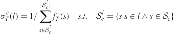 (5.3)
(5.3)
As an illustrative example, Figure 5.7 shows the computed minimum regional sensor support values for the smart home used in our experiments.
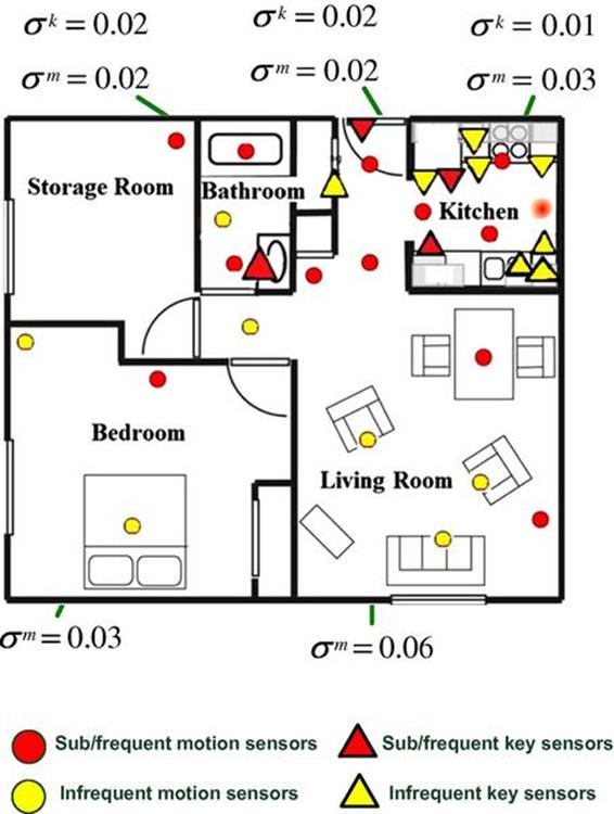
FIGURE 5.7 The frequent/subfrequent sensors are selected based on the minimum regional support, instead of a global support.
Using the minimum regional sensor frequencies, frequent and subfrequent sensors are defined as follows.
Definition 5.2 Let ![]() be a sensor of category
be a sensor of category ![]() located in location
located in location ![]() . The frequency of
. The frequency of ![]() over a time period
over a time period ![]() , denoted by
, denoted by ![]() , is the number of times in time period
, is the number of times in time period ![]() in which
in which ![]() occurs. The support of
occurs. The support of ![]() in location
in location ![]() and over time period
and over time period ![]() is
is ![]() divided by the total number of sensor events of the same category occurring in
divided by the total number of sensor events of the same category occurring in ![]() during
during ![]() . Let
. Let ![]() be the maximum sensor support error. Sensor
be the maximum sensor support error. Sensor ![]() is said to be frequent if its support is no less than
is said to be frequent if its support is no less than ![]() . It is subfrequent if its support is less than
. It is subfrequent if its support is less than ![]() , but no less than
, but no less than ![]() ; otherwise, it is infrequent.
; otherwise, it is infrequent.
Only the sensor events from the frequent and subfrequent sensors are added to the reduced batch ![]() , which is then used for constructing longer sequences. We use a pattern growth method that grows a pattern by its prefix and suffix [51]. To account for the variations in the patterns, the concept of a general pattern is introduced. A general pattern is a set of all the variations that have a similar structure in terms of comprising sensor events but have different event orders [54].
, which is then used for constructing longer sequences. We use a pattern growth method that grows a pattern by its prefix and suffix [51]. To account for the variations in the patterns, the concept of a general pattern is introduced. A general pattern is a set of all the variations that have a similar structure in terms of comprising sensor events but have different event orders [54].
During pattern growth, if an already-discovered variation matches a newly discovered pattern, its frequency and continuity information are updated. If the newly discovered pattern matches the general pattern, but does not exactly match any of the variations, it is added as a new variation. Otherwise, it is considered a new general pattern.
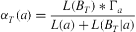
At the end of each pattern growth iteration, infrequent or highly discontinuous patterns and variations are discarded as uninteresting patterns. Instead of solely using a pattern’s frequency as a measure of interest, we use a compression objective based on the minimum description length (MDL) [55]. Using a compression objective allows us to take into account the ability of the pattern to compress a dataset with respect to the pattern’s length and continuity. The compression value of a general pattern ![]() over a time period
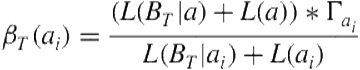
over a time period ![]() is defined in Equation 5.4. The compression value of a variation
is defined in Equation 5.4. The compression value of a variation ![]() of a general pattern over a time period
of a general pattern over a time period ![]() is defined in Equation 5.5.
is defined in Equation 5.5.
Here, ![]() refers to the description length as defined by the MDL principle, and
refers to the description length as defined by the MDL principle, and ![]() refers to continuity as defined in Rashidi et al. [54]. Continuity basically shows how contiguous the component events of a pattern or a variation are. It is computed in a bottom-up manner, such that for the variation continuity is defined in terms of the average number of infrequent sensor events separating each two successive events of the variation. The continuity between each two events of a pattern instance is defined in terms of the average number of the infrequent events separating the two events. The more the separation between the two events, the less is the continuity. For a pattern variation, the continuity is based on the average continuity of its instances. For a general pattern the continuity is defined as the average continuity of its variations.
refers to continuity as defined in Rashidi et al. [54]. Continuity basically shows how contiguous the component events of a pattern or a variation are. It is computed in a bottom-up manner, such that for the variation continuity is defined in terms of the average number of infrequent sensor events separating each two successive events of the variation. The continuity between each two events of a pattern instance is defined in terms of the average number of the infrequent events separating the two events. The more the separation between the two events, the less is the continuity. For a pattern variation, the continuity is based on the average continuity of its instances. For a general pattern the continuity is defined as the average continuity of its variations.
 (5.4)
(5.4)
 (5.5)
(5.5)
Variation compression measures the capability of a variation to compress a general pattern compared to the other variations. Compression of a general pattern shows the overall capability of it to compress the dataset with respect to its length and continuity. Based on using the compression values and by using a maximum compression error, we define interesting, subinteresting, and uninteresting patterns and variations.
Definition 5.3 Let the compression of a general pattern ![]() be defined as in Equation 5.4 over a time period
be defined as in Equation 5.4 over a time period ![]() . Also let
. Also let ![]() and
and ![]() denote the minimum compression and maximum compression error. The general pattern
denote the minimum compression and maximum compression error. The general pattern ![]() is said to be interesting if its compression
is said to be interesting if its compression ![]() is no less than
is no less than ![]() . It is subinteresting if its compression is less than
. It is subinteresting if its compression is less than ![]() , but no less than
, but no less than ![]() ; otherwise, it is uninteresting.
; otherwise, it is uninteresting.
We also give a similar definition for identifying interesting/subinteresting variations of a pattern. Let the average variation compression of all variations of a general pattern ![]() over a time period
over a time period ![]() be defined as in Equation 5.6. Here, the number of variations of a general pattern is denoted by
be defined as in Equation 5.6. Here, the number of variations of a general pattern is denoted by ![]() .
.
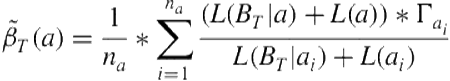 (5.6)
(5.6)
Definition 5.4 Let the compression of a variation ![]() of a general pattern
of a general pattern ![]() be defined as in Equation 5.5 over a time period
be defined as in Equation 5.5 over a time period ![]() . Also let
. Also let ![]() denote the maximum variation compression error. A variation
denote the maximum variation compression error. A variation ![]() is said to be interesting over a time period
is said to be interesting over a time period ![]() if its compression
if its compression![]() is no less than
is no less than ![]() . It is subinteresting if its compression is less than
. It is subinteresting if its compression is less than ![]() , but no less than
, but no less than ![]() ; otherwise, it is uninteresting.
; otherwise, it is uninteresting.
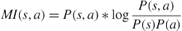
During each pattern-growth iteration, based on the previous definitions, the uninteresting patterns and variations, that is, those that are either highly discontinuous or infrequent (with respect to their length) are pruned. We also prune redundant nonmaximal general patterns, that is, those patterns that are totally contained in another larger pattern. To only maintain the very relevant variations of a pattern, irrelevant variations of a pattern also are discarded based on using mutual information [24] as in Equation 5.7. It allows us to find core sensors for each general pattern ![]() .
.
Finding the set of core sensors allows us to prune the irrelevant variations of a pattern that does not contain the core sensors. Here, ![]() is the joint probability distribution of a sensor
is the joint probability distribution of a sensor ![]() and general pattern
and general pattern ![]() , while
, while ![]() and
and ![]() are the marginal probability distributions. A high mutual information value indicates that the sensor is a core sensor.
are the marginal probability distributions. A high mutual information value indicates that the sensor is a core sensor.
 (5.7)
(5.7)
We continue extending the patterns by prefix and suffix at each iteration until no more interesting patterns are found. A postprocessing step records attributes of the patterns (e.g., event durations and start times). We refer to the pruning process performed during the pattern growth on the current data batch as normal pruning. Note that it is different from the tail-pruning process performed on the tilted-time window to discard the unpromising patterns over time.
In the following subsection we describe how the tilted-time window is updated after discovering patterns of the current data batch.
5.3.4 Updating the Tilted-Time Window
After discovering the patterns in the current data batch as described in the previous subsection, the tilted-time window will be updated; each general pattern is associated with it. The tilted-time window keeps track of the general pattern’s history as well as its variations. Whenever a new batch arrives, after discovering its interesting general patterns, we replace the compressions at the finest level of granularity with the recently computed compressions. If a variation of a general pattern is not observed in the current batch, we set its recent compression to ![]() . If none of the variations of a general pattern are perceived in the current batch, then the general pattern’s recent compression is also set to
. If none of the variations of a general pattern are perceived in the current batch, then the general pattern’s recent compression is also set to ![]() .
.
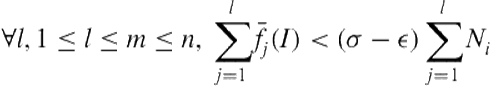
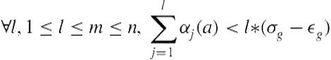
To reduce the number of maintained records and to remove unpromising general patterns, we use the following tail-pruning mechanisms as an extension of the original tail-pruning method in [20]. Let ![]() denote the computed compression of general pattern
denote the computed compression of general pattern ![]() in time unit
in time unit ![]() . Also let
. Also let ![]() refer to the most recent time point. For some
refer to the most recent time point. For some ![]() , where
, where ![]() , the compression records
, the compression records ![]() are pruned if Equations 5.8 and 5.9 hold.
are pruned if Equations 5.8 and 5.9 hold.
![]() (5.8)
(5.8)
 (5.9)
(5.9)
Equation 5.8 finds a point ![]() in the stream, such that before that point the computed compression of the general pattern
in the stream, such that before that point the computed compression of the general pattern ![]() is always less than the minimum compression required. Equation 5.9 computes the time unit
is always less than the minimum compression required. Equation 5.9 computes the time unit ![]() , where
, where ![]() , such that before that point the sum of the computed compression of
, such that before that point the sum of the computed compression of ![]() is always less than the relaxed minimum compression threshold. In this case, the compression records of
is always less than the relaxed minimum compression threshold. In this case, the compression records of ![]() from
from ![]() to
to ![]() are considered unpromising and are pruned.
are considered unpromising and are pruned.
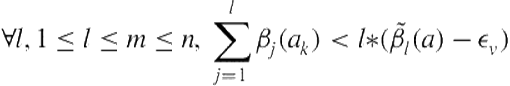
We define a similar procedure for pruning the variations of a general pattern. We prune a variation ![]() if the conditions in Equations 5.10 and 5.11 hold.
if the conditions in Equations 5.10 and 5.11 hold.
![]() (5.10)
(5.10)
 (5.11)
Equation 5.10 finds a point in time where the computed compression of a variation is less than the average computed compression of all variations in that time unit. Equation 5.11 computes the time unit ![]() , where
, where ![]() , such that before that point the sum of the computed compression of
, such that before that point the sum of the computed compression of ![]() is always less than the relaxed minimum support threshold. In this case, the compression records of
is always less than the relaxed minimum support threshold. In this case, the compression records of ![]() from
from ![]() to
to ![]() are considered unpromising and are pruned.
are considered unpromising and are pruned.
5.4 Experiments
The performance of the system was evaluated on the data collected from two smart apartments. The layout of the apartments including sensor placement and location tags, as well as the activity diagrams, are shown in Figure 5.8. We refer to the apartments inFigures 5.8a and 5.8b as Apartment 1 and Apartment 2. The apartments were equipped with infrared motion sensors installed on ceilings, infrared area sensors installed on the walls, and switch contact sensors to detect the open/close status of the doors and cabinets. The data were collected during ![]() weeks for Apartment 1 and 19 weeks for Apartment 2.
weeks for Apartment 1 and 19 weeks for Apartment 2.
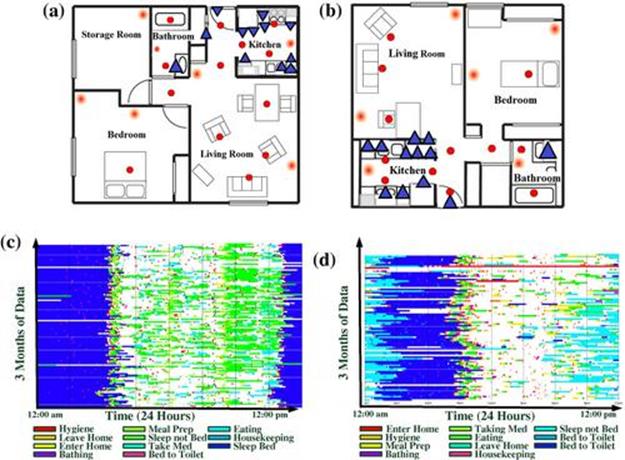
FIGURE 5.8 Sensor map and location tags for each apartment. On the map, circles show motion sensors while triangles show switch contact sensors. (a) Apartment 1 layout; (b) Apartment 2 layout; (c) Apartment 1 activity diagram; (d) Apartment 2 activity diagram.
During the data-collection period, the resident of Apartment 2 was away for approximately 20 days, once during day 12 and once during day 17. Also the last week of data collection in both apartments does not include a full cycle. In our experiments, we constrain each batch to contain approximately one week of data. In our experiments, we set the maximum errors ![]() , and
, and ![]() to
to ![]() , as suggested in the literature [20]. Also
, as suggested in the literature [20]. Also ![]() was set to
was set to ![]() based on several runs of experiments.
based on several runs of experiments.
To be able to evaluate the results of our algorithms based on a ground truth, each one of the datasets was annotated with activities of interest. A total of 10 activities were noted for each apartment, including bathing, bed-toilet transition, eating, leave home/enter home, housekeeping, meal preparation (cooking), personal hygiene, sleeping in bed, sleeping not in bed (relaxing), and taking medicine. Note that in our annotated datasets, each sensor event has an activity label as part of it. The activity label also can be “None,” if a sensor event does not belong to any of the preceding activities.
To validate the results, we consider each discovered pattern by our system as representing one activity; therefore, all of its sensor events, or at least a high proportion of them, should have homogenous activity labels according to the ground truth annotations. In practice, if a certain percentage of the sensor events (e.g., ![]() ) have the same activity label
) have the same activity label ![]() , we can say that our system has recovered the pattern
, we can say that our system has recovered the pattern ![]() .
.
Apartment 1 includes 193,592 sensor events and 3384 annotated activity instances. Apartment 2 includes 132,550 sensor events and 2602 annotated activity instances. Figures 5.9a and 5.9b show the number of recorded sensor events over time. As we mentioned, the resident of Apartment 2 was not at home during two different time periods; thus, we can see the gaps in Figure 5.9b.
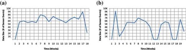
FIGURE 5.9 Total number of recorded sensor events over time (time unit = weeks). (a) Apartment 1; (b) Apartment 2.
We ran our algorithms on both apartments’ datasets. Figures 5.10a and 5.10b show the number of distinct discovered patterns over time based on using a global support (the approach used by DVSM) versus using multiple regional support (the approach used by Stream/COM). The results show that by using multiple regional support, we are able to detect a higher percentage of interesting patterns. Some of the patterns that have not been discovered are indeed quite difficult to spot and in some cases also less frequent. For example, the housekeeping activity happens every 2 to 4 weeks and is not associated with any specific sensor. Also some of the similar patterns are merged together, as they use the same set of sensors (e.g., eating and relaxing activities).
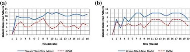
FIGURE 5.10 Total number of distinct discovered patterns over time. (a) Apartment 1 (time unit = weeks); (b) Apartment 2 (time unit = weeks).
It should be noted that some of the activities are discovered multiple times in the form of different patterns, as the activity might be performed with a different motion trajectory using different sensors. One also can see that the number of discovered patterns increases at the beginning and then is adjusted over time depending on the perceived patterns in the data. The number of discovered patterns depends on perceived patterns in the current data batch and previous batches, as well as the compression of patterns in tilted-time window records. Therefore, some of the patterns might disappear and reappear over time, showing how consistently the resident performs those activities.
To reduce the number of discovered patterns over time, our algorithm performs two types of pruning. The first type, normal pruning, prunes patterns and variations while processing the current data batch. The second type, tail pruning, discards unpromising patterns and variations stored in all tilted-time windows. Figures 5.11a and 5.11b show the results of both types of pruning on the first dataset. Figures 5.11d and 5.11e show the results of both types of pruning on the second dataset. Figures 5.11c and 5.11f show the tail-pruning results in the tilted-time window over time. Note that the gaps for Apartment 2 results are due to the ![]() days when the resident was away. Also, Figures 5.11b and 5.11e show the declining trend of number of pruned patterns over time, as the straight trend line indicates.
days when the resident was away. Also, Figures 5.11b and 5.11e show the declining trend of number of pruned patterns over time, as the straight trend line indicates.
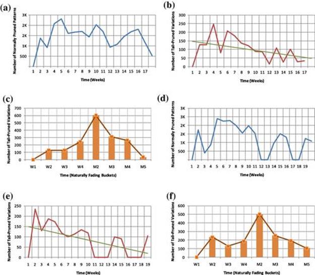
FIGURE 5.11 Total number of tail-pruned variations and normally pruned patterns over time. For the bar charts, W1–W4 refer to weeks 1 through 4, and M2–M5 refer to months 2 through 5. (a) Apartment 1 (time unit = weeks); (b) Apartment 1 (time unit = weeks); (c) Apartment 1 (time unit = tilted-time frame); (d) Apartment 1 (time unit = weeks); (e) Apartment 2 (time unit = weeks); (f) Apartment 2 (time unit = tilted-time frame).
By comparing the results of normal pruning in Figures 5.11a and 5.11d against the number of recorded sensors in Figures 5.9a and 5.9b, one can see that the normal pruning somehow follows the pattern of recorded sensors. If more sensor events were available, more patterns would be obtained and more patterns would be pruned. For the tail-pruning results, depicted in Figures 5.11b, 5.11e, 5.11c, and 5.11f, the number of tail-pruned patterns at first increases in order to discard the many unpromising patterns at the beginning. Then the number of tail-pruned patterns decreases over time as the algorithm stabilizes.
We have developed a visualization software that allows us to visualize the patterns and variations along with their statistics, as depicted in Figure 5.12. Figure 5.12b shows a taking medication activity in Apartment ![]() that was pruned at the third week due to its low compression. Figure 5.12c shows two variations of the leave home activity pattern in Apartment
that was pruned at the third week due to its low compression. Figure 5.12c shows two variations of the leave home activity pattern in Apartment ![]() . Note that we use color coding to differentiate between different variations if multiple variations are shown simultaneously. Figure 5.12e shows the meal preparationpattern in Apartment
. Note that we use color coding to differentiate between different variations if multiple variations are shown simultaneously. Figure 5.12e shows the meal preparationpattern in Apartment ![]() .
.
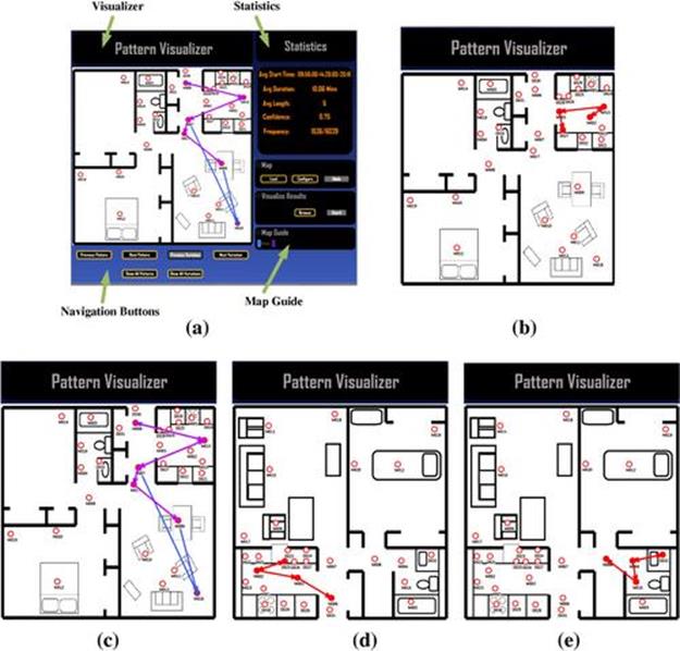
FIGURE 5.12 Visualization of patterns and variations. (a) Pattern Visualizer; (b) The taking medication pattern in Apartment 1; (c) Two variations of the leave home pattern in Apartment 1; (d) The meal preparation pattern in Apartment 2; (e) The personal hygiene pattern in Apartment 2.
To illustrate the changes of a specific pattern over time, we show the results of our algorithm for the taking medication activity over time. Figure 5.13a shows the number of discovered variations over time for the taking medication activity. Figure 5.13b shows the same results in the tilted-time window over time. We can clearly see that the number of discovered variations quickly drops due to the tail-pruning process. This shows that despite the fact that we are maintaining time records over time for all variations, many of the uninteresting, unpromising, and irrelevant variations are pruned over time, making our algorithm more efficient in practice.
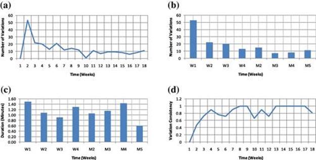
FIGURE 5.13 Number of discovered variations, duration, and consistency for the taking medication activity pattern over time. (a) Number of discovered variations (time unit = weeks); (b) Number of discovered variations (time unit = tilted-time frame); (c) Duration (time unit = weeks); (d) Variation consistency (time unit = weeks).
We also show how the average duration of the taking medication pattern changes over time in Figure 5.13c. Presenting such information can be informative to caregivers to detect any anomalous events in the patterns. Figure 5.13d shows the consistency of the taking medication variations over time. Similar to the results obtained for the average variation consistency of all patterns, we see that the variation consistency increased and then stabilized quickly.
In summary, the results of our experiments confirm that we can find sequential patterns from a steam of sensor data over time. It also shows that using two types of pruning techniques allows for a large number of unpromising, uninteresting, and irrelevant patterns and variations to be discarded to achieve a more efficient solution that can be used in practice.
5.5 Conclusion
This chapter reviewed the state-of-the-art unsupervised methods for activity recognition. In particular, we described a scalable activity discovery and recognition method for complex large real-world datasets based on sequential data mining and stream data mining methods. Most current approaches use supervised methods for activity recognition. However, due to the required effort and time for annotating activity datasets, supervised methods do not scale up well in practice. This chapter shows an approach to automatically discover activity patterns and their variations from streaming data, even if the patterns exhibit discontinuity or if the patterns’ frequencies exhibit differences across various regions in a home.
We believe that, in general, unsupervised activity discovery methods can have many implications for future applications. For example, in the case of smart homes, stream mining methods promise automation of large-scale deployments without any need for human annotation. Also, stream mining methods can be used to reveal new activity patterns over time and to help us understand changes in activity patterns. Besides activity mining, our discontinuous and varied-order stream mining method can be useful in other application domains, where different variations of a pattern can reveal useful information—for example, Web-click mining. Also, our proposed solution for solving the problem of rare items in a datastream can be applied to domains such as Web-click mining. For example, certain Web pages might have a lower chance of being visited by visitors, but we still might be interested in finding click patterns in such pages.
We suggest several new directions for future research on sequence stream mining methods in the context of activity recognition applications. One direction is to combine background knowledge with stream sequence mining to leverage activity recognition. Another direction is to benefit from parallel and distributed implementation in order to speed up the algorithms. Finally, we envision that progress in sensor development will allow us to fuse activity knowledge with many other types of information such as health-related data or environmental information. This ultimately will allow us to model our surroundings more accurately in an autonomous manner.
References
1. Abowd G, Mynatt E. Designing for the human experience in smart environments. In: Cook DJ, Das SK, eds. Smart environments: technology, protocols, and applications. Wiley; 2004:153-174.
2. Agrawal R, Imieliński T, Swami A. Mining association rules between sets of items in large databases. Proceedings of the ACM SIGMOD International Conference on Management of Data. 1993:207-216.
3. Agrawal R, Srikant R. Mining sequential patterns. ICDE ’95: Proceedings of the 11th International Conference on Data Engineering. 1995:3-14.
4. Ahmadi A, Rowlands D, James D. Investigating the translational and rotational motion of the swing using accelerometers for athlete skill assessment. IEEE Conference on Sensors. 2006:980-983.
5. Ayres J, Flannick J, Gehrke J, Yiu T. Sequential pattern mining using a bitmap representation. Proceedings of the Eighth ACM SIGKDD International Conference on Knowledge Discovery and Data Mining. 2002:429-435.
6. Barger T, Brown D, Alwan M. Health-status monitoring through analysis of behavioral patterns. IEEE Trans Syst Man Cybern Part A: Syst Hum. 2005;35(1):22-27.
7. Bouchard B, Giroux S, Bouzouane A. A keyhole plan recognition model for Alzheimer patients: first results. Appl Artif Intell. 2007;21:623-658.
8. Brdiczka O, Maisonnasse J, Reignier P. Automatic detection of interaction groups. Proceedings of the Seventh International Conference on Multimodal Interfaces. 2005:32-36.
9. Chang JH, Lee WS. Finding recent frequent itemsets adaptively over online data streams. Proceedings of the Ninth ACM SIGKDD International Conference on Knowledge Discovery and Data Mining. 2003:487-492.
10. Chen G, Wu X, Zhu X. Sequential pattern mining in multiple streams. ICDM ’05: Proceedings of the Fifth IEEE International Conference on Data Mining. 2005:585-588.
11. Cheng J, Ke Y, Ng W. A survey on algorithms for mining frequent itemsets over data streams. Knowl Inform Syst. 2008;16(1):1-27.
12. Cook D, Das S. Smart environments: technology, protocols and applications. Wiley series on parallel and distributed computing. Wiley-Interscience; 2004.
13. Cook D, Schmitter-Edgecombe M. Assessing the quality of activities in a smart environment. Method Inform Med. 2009;48(05):480-485.
14. Cook D, Youngblood M, Heierman EOI, et al. Mavhome: an agent-based smart home. IEEE International Conference on Pervasive Computing and Communications. 2003:521-524.
15. Curtis DW, Pino EJ, Bailey JM, Shih EI, Waterman J, Vinterbo SA, et al. Smart: an integrated wireless system for monitoring unattended patients. J Am Med Inform Assoc. 2008;15(1):44-53.
16. Dimitrov T, Pauli J, Naroska E. Unsupervised recognition of ADLs. In: Konstantopoulos S, Perantonis S, Karkaletsis V, Spyropoulos C, Vouros G, eds. Artificial intelligence: theories, models and applications. Lecture notes in computer science. vol. 6040. Springer; 2010:71-80.
17. Doctor F, Hagras H, Callaghan V. A fuzzy embedded agent-based approach for realizing ambient intelligence in intelligent inhabited environments. IEEE Trans Syst Man Cybern Syst Hum. 2005;35(1):55-65.
18. Fu Li H, Yin Lee S, Kwan Shan M. An efficient algorithm for mining frequent itemsets over the entire history of data streams. First International Workshop on Knowledge Discovery in Data Streams. 2004:45-55.
19. Garofalakis M, Gehrke J, Rastogi R. Querying and mining data streams: you only get one look a tutorial. Proceedings of the ACM SIGMOD International Conference on Management of Data. 2002:635.
20. Giannella C, Han J, Pei J, Yan X, Yu P. Mining frequent patterns in data streams at multiple time granularities. Next Gen Data Min. 2003;212:191-212.
21. Gopalratnam K, Cook DJ. Online sequential prediction via incremental parsing: the active LeZi algorithm. IEEE Intell Syst. 2007;22(1):52-58.
22. Gu T, Wang L, Wu Z, Tao X, Lu J. A pattern mining approach to sensor-based human activity recognition. IEEE Trans Knowl Data Eng. 2011:1.
23. Gu T, Wu Z, Tao X, Pung H, Lu J. Epsicar: an emerging patterns based approach to sequential, interleaved and concurrent activity recognition. International Conference on Pervasive Computing and Communication. 2009:1-9.
24. Guyon I, Elisseeff A. An introduction to variable and feature selection. Mach Learn Res. 2003;3:1157-1182.
25. Han J, Chen Y, Dong G, et al. Stream cube: an architecture for multi-dimensional analysis of data streams. Distrib Parall Dat. 2005;18(2):173-197.
26. Han J, Pei J, Mortazavi-Asl B, Chen Q, Dayal U, Hsu M-C. Freespan: frequent pattern-projected sequential pattern mining. Proceedings of the Sixth ACM SIGKDD International Conference on Knowledge Discovery and Data Mining. 2000:355-359.
27. Hayes TL, Pavel M, Larimer N, Tsay IA, Nutt J, Adami AG. Distributed healthcare: simultaneous assessment of multiple individuals. IEEE Pervas Comput. 2007;6(1):36-43.
28. Heierman III EO, Cook DJ. Improving home automation by discovering regularly occurring device usage patterns. In: ICDM ’03: Proceedings of the Third IEEE International Conference on Data Mining; 2003. p. 537.
29. Hensel B, Demiris G, Courtney K. Defining obtrusiveness in home telehealth technologies: a conceptual framework. J Am Med Inform Assoc. 2006;13(4):428-431.
30. Huynh T, Schiele B. Towards less supervision in activity recognition from wearable sensors. Proceedings of the 10th IEEE International Symposium on Wearable Computers. 2006:3-10.
31. Liao L, Fox D, Kautz H. Location-based activity recognition using relational Markov networks. Proceedings of the International Joint Conference on Artificial Intelligence. 2005:773-778.
32. Liu B, Hsu W, Ma Y. Mining association rules with multiple minimum supports. Proceedings of the Fifth ACM SIGKDD International Conference on Knowledge Discovery and Data Mining. 1999:337-341.
33. Lorincz K, Chen B-R, Challen GW, et al. Mercury: a wearable sensor network platform for high-fidelity motion analysis. ACM Conference on Embedded Networked Sensor Systems. 2009:183-196.
34. Lorincz K, Malan DJ, Fulford-Jones TRF, Nawoj A, Clavel A, Shnayder V, et al. Sensor networks for emergency response: challenges and opportunities. IEEE Pervas Comput. 2004;3(4):16-23.
35. Mahajan D, Kwatra N, Jain S, Kalra P, Banerjee S. A framework for activity recognition and detection of unusual activities. Indian Conference on Computer Vision, Graphics and Image Processing. 2004:15-21.
36. Manku GS, Motwani R. Approximate frequency counts over data streams. Proceedings of the 28th International Conference on Very Large Data Bases. 2002:346-357.
37. Marascu A, Masseglia F. Mining sequential patterns from data streams: a centroid approach. J Intell Inform Syst. 2006;27(3):291-307.
38. Masseglia F, Cathala F, Poncelet P. The PSP approach for mining sequential patterns. Proceedings of the Second European Symposium on Principles of Data Mining and Knowledge Discovery. 1998:176-184.
39. Maurer U, Smailagic A, Siewiorek D, Deisher M. Activity recognition and monitoring using multiple sensors on different body positions. International Workshop on Wearable and Implantable Body Sensor Networks. 2006:4-116.
40. Michahelles F, Schiele B. Sensing and monitoring professional skiers. IEEE Pervas Comput. 2005;4(3):40-46.
41. Ogris G, Stiefmeier T, Lukowicz P, Troster G. Using a complex multi-modal on-body sensor system for activity spotting. IEEE International Symposium on Wearable Computers. 2008:55-62.
42. Palmes P, Pung HK, Gu T, Xue W, Chen S. Object relevance weight pattern mining for activity recognition and segmentation. Pervas Mob Comput. 2010;6:43-57.
43. Pei J, Han J, Mortazavi-Asl B, et al. Prefixspan: mining sequential patterns by prefix-projected growth. Proceedings of the 17th International Conference on Data Engineering. 2001:215-224.
44. Pei J, Han J, Wang W. Constraint-based sequential pattern mining: the pattern-growth methods. J Intell Inform Syst. 2007;28(2):133-160.
45. Pentland AS. Healthwear: medical technology becomes wearable. Computer. 2004;37(5):42-49.
46. Perkowitz M, Philipose M, Fishkin K, Patterson DJ. Mining models of human activities from the web. Proceedings of the 13th International Conference on World Wide Web. 2004:573-582.
47. Philipose M, Fishkin KP, Perkowitz M, et al. Inferring activities from interactions with objects. IEEE Pervas Comput. 2004;3(4):50-57.
48. Raïssi C, Plantevit M. Mining multidimensional sequential patterns over data streams. DaWaK ’08: Proceedings of the 10th International Conference on Data Warehousing and Knowledge Discovery. 2008:263-272.
49. Raïssi C, Poncelet P, Teisseire M. Need for speed: mining sequential pattens in data streams. BDA05: Actes des 21iemes Journees Bases de Donnees Avancees. 2005:1-11.
50. Rashidi P, Cook DJ. Adapting to resident preferences in smart environments. AAAI Workshop on Preference Handling. 2008:78-84.
51. Rashidi P, Cook DJ. The resident in the loop: adapting the smart home to the user. IEEE Trans Syst Man Cybern J, Part A. 2009;39(5):949-959.
52. Rashidi P, Cook DJ. Mining and monitoring patterns of daily routines for assisted living in real world settings. Proceedings of the First ACM International Health Informatics Symposium. 2010:336-345.
53. Rashidi P, Cook DJ. Mining sensor streams for discovering human activity patterns over time. IEEE International Conference on Data Mining. 2010:431-440.
54. Rashidi P, Cook DJ, Holder LB, Schmitter-Edgecombe M. Discovering activities to recognize and track in a smart environment. IEEE Trans Knowl Data Eng. 2010;23(4):527-539.
55. Rissanen J. Modeling by shortest data description. Automatica. 1978;14:465-471.
56. Salarian A, Russmann H, Vingerhoets F, et al. Gait assessment in Parkinson’s disease: Toward an ambulatory system for long-term monitoring. IEEE Trans Biomed Eng. 2004;51(8):1434-1443.
57. Sánchez D, Tentori M, Favela J. Activity recognition for the smart hospital. IEEE Intell Syst. 2008;23(2):50-57.
58. Schiele B. Unsupervised discovery of structure in activity data using multiple eigenspaces. Second International Workshop on Location and Context Awareness. 2006:151-167.
59. Song Y, Lasecki W, Bigham J, Kautz H. Training activity recognition systems online using real-time crowdsourcing. UbiComp. 2012:1-2.
60. Stauffer C, Grimson W. Learning patterns of activity using real-time tracking. IEEE Trans Pattern Anal Mach Intell. 2000;22(8):747-757.
61. Tapia EM, Intille SS, Larson K. Activity recognition in the home using simple and ubiquitous sensors. Pervas Comput. 2004;3001:158-175.
62. Teng W-G, Chen M-S, Yu PS. A regression-based temporal pattern mining scheme for data streams. Proceedings of the 29th International Conference on Very Large Data Bases. 2003:93-104.
63. Nguyen T, Phung D, Gupta S, Venkatesh S. Extraction of latent patterns and contexts from social honest signals using hierarchical Dirichlet processes. PerCom. 2013:47-55.
64. Vahdatpour A, Amini N, Sarrafzadeh M. Toward unsupervised activity discovery using multi-dimensional motif detection in time series. Proceedings of the 21st International Joint Conference on Artificial Intelligence. 2009:1261-1266.
65. van Kasteren T, Krose B. Bayesian activity recognition in residence for elders. Third IET International Conference on Intelligent Environments. 2007:209-212.
66. Wang J, Han J. Bide: efficient mining of frequent closed sequences. Proceedings of the 20th International Conference on Data Engineering. 2004:79.
67. Wren C, Munguia-Tapia E. Toward scalable activity recognition for sensor networks. Proceedings of the Workshop on Location and Context-Awareness. 2006:218-235.
68. Wyatt D, Philipose M, Choudhury T. Unsupervised activity recognition using automatically mined common sense. Proceedings of the 20th National Conference on Artificial Intelligence, Vol. 1. 2005:21-27.
69. Yin J, Yang Q, Pan JJ. Sensor-based abnormal human-activity detection. IEEE Trans Knowl Data Eng. 2008;20(8):1082-1090.
70. Yiping T, Shunjing J, Zhongyuan Y, Sisi Y. Detection elder abnormal activities by using omni-directional vision sensor: activity data collection and modeling. SICE-ICASE: Proceedings of the International Joint Conference. 2006:3850-3853.
71. Zaki MJ. Spade: an efficient algorithm for mining frequent sequences. Mach Learn. 2001;42:31-60.
72. Zhao L, Sukthankar G, Sukthankar R. Incremental relabeling for active learning with noisy crowdsourced annotations. Privacy, Security, Risk and Trust (Passat)—Third International Conference on IEEE Third International Conference on Social Computing. 2011:728-733.
73. Zhao L, Wang X, Sukthankar G, Sukthankar R. Motif discovery and feature selection for crf-based activity recognition. Proceedings of the 20th International Conference on Pattern Recognition. 2010:3826-3829.
74. Zheng VW, Zheng Y, Xie X, Yang Q. Collaborative location and activity recommendations with GPS history data. Proceedings of the 19th International Conference on World Wide Web. 2010:1029-1038.
1 Based on data collected from Center for Advanced Studies in Adaptive System (CASAS) testbeds [54].
2 A preliminary version of this method appeared in the 2010 ICDM Proceedings; see Rashid and Cook [53].