Plan, Activity, and Intent Recognition: Theory and Practice, FIRST EDITION (2014)

Part II. Activity Discovery and Recognition

Chapter 6. Learning Latent Activities from Social Signals with Hierarchical Dirichlet Processes

Dinh Phung, Thuong Nguyen, Sunil Gupta and Svetha Venkatesh, Deakin University, Waurn Ponds, VIC, Australia

Abstract

Understanding human activities is an important research topic, most noticeably in assisted-living and healthcare monitoring environments. Beyond simple forms of activity (e.g., an RFID event of entering a building), learning latent activities that are more semantically interpretable, such as sitting at a desk, meeting with people, or gathering with friends, remains a challenging problem. Supervised learning has been the typical modeling choice in the past. However, this requires labeled training data, is unable to predict never-seen-before activity, and fails to adapt to the continuing growth of data over time. In this chapter, we explore the use of a Bayesian nonparametric method, in particular the hierarchical Dirichlet process, to infer latent activities from sensor data acquired in a pervasive setting. Our framework is unsupervised, requires no labeled data, and is able to discover new activities as data grows. We present experiments on extracting movement and interaction activities from sociometric badge signals and show how to use them for detecting of subcommunities. Using the popular Reality Mining dataset, we further demonstrate the extraction of colocation activities and use them to automatically infer the structure of social subgroups.

Keywords

Activity recognition

Bayesian nonparametric

Hierarchical Dirichlet process

Pervasive sensors

Healthcare monitoring

6.1 Introduction

The proliferation of pervasive sensing platforms for human computing and healthcare has deeply transformed our lives. Building scalable activity-aware applications that can learn, act, and behave intelligently has increasingly become an important research topic. The ability to discover meaningful and measurable activities are crucial to this endeavor. Extracting and using simple forms of activity, such as spatial whereabouts or radio frequency identification (RFID) triggers of entering a building, have remained the focus of much existing work in context-aware applications (e.g, see a recent survey in Bettini et al. [5] and Dey [16]). In most cases, these activities can be readily derived from the recorded raw signals—geolocation from GPS, colocation with known people from Bluetooth, or the presence/absence of someone from a meeting room using RFID tags, though they might be susceptible to changes without careful data cleaning and processing when data grows [5].

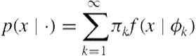
Beyond these simple forms of activity, learning latent activities that are more semantically interpretable, which cannot be trivially derived from the signals, remains a challenging problem. We call these latent activities. For example, instead of using raw coordinate readings from the accelerometer sensor, we consider the user’s movement status such as walking or running; or instead of using GPS longitude/latitude readings, one may want to learn high-level daily rhythms from the GPS data [52].

Inferring latent activities is a challenging task that has received little research attention. Most of the existing approaches have used parametric methods from machine learning and data mining. Standard supervised learning and unsupervised learning techniques are the most popular ones used. These include Support Vector Machines (SVMs), Naive Bayes, and hidden Markov models (HMM), to name a few. Typical unsupervised learning methods include Gaussian mixture models (GMM), K-means, and latent Dirichlet allocation (LDA) (see Section 6.2). These methods are parametric models in the sense that, once models are learned from a particular dataset, they are fixed and unable to grow or expand as the data grow.

A more severe drawback of these methods is the need to specify the number of latent activities in advance, thus limiting the model to a predefined set of activities. For example, one needs to specify the number of clusters for GMM, the number of states for HMM, or the number of topics for LDA. It is often difficult in practice to specify these parameters in the first place. A common strategy is to perform model selection, searching through the parameter space to pick the best performance on a held-out dataset, which can be cumbersome, computationally inefficient, and sensitive to the held-out dataset. These parametric methods are potentially unsuitable for ubiquitous applications, such as in pervasive health, as the data are typically growing over time and have “no clear beginning and ending” [1].

This chapter addresses these problems by proposing the use of Bayesian nonparametric (BNP) methods, a recent data modeling paradigm in machine learning, to infer latent activities from sensor data acquired in a pervasive setting with an emphasis on social signals. These Bayesian models specify a nonparametric prior on the data-generative process; as such, they allow the number of latent activities to be learned automatically and grow with the data, thus overcoming the fundamental difficulty of model selection encountered in the aforementioned parametric models.

In particular, we employ the hierarchical Dirichlet process (HDP) [62], a recent BNP model designed for modeling grouped data (e.g., a collection of documents, images, or signals) represented in appropriate form. Similar to other Bayesian nonparametric models, HDP automatically infers the number of latent topics—equivalent to our latent activities—from data and assigns each data point to a topic; thus, HDP simultaneously discovers latent activities and assigns a mixture proportion to each document (or a group of signals), which can be used as a latent feature representation for users’ activities for additional tasks such as classification or clustering.

We demonstrate the framework on the collection of social signals, a new type of data-sensing paradigm and network science pioneered at the MIT Media Lab [50]. We experiment with two datasets. The first was collected in our lab using sociometric badges provided by Sociometric Solutions.¹ The second one is the well-known Reality Mining dataset [20]. For the sociometric data, we report two experiments: discovering latent movement activities derived from accelerometer data and colocation activities from Bluetooth data.

To demonstrate the feasibility of the framework in a larger setting, we experiment with the Reality Mining dataset and discover the interaction activities from this data. In all cases, to demonstrate the strength of Bayesian nonparametric frameworks, we also compare our results with activities discovered by latent Dirichlet allocation [7]—a widely acknowledged state-of-the-art parametric model for topic modeling. We derive the similarity between subjects in our study using latent activities discovered, then feed the similarity to a clustering algorithm and compare the performance between the two approaches. We quantitatively judge the clustering performance on four metrics commonly used in information retrieval and data mining: F-measure, Rand index, purity, and normalized mutual information (NMI). Without the need of searching over the parameter space, HDP consistently delivers results comparable with the best performance of LDA, up to 0.9 in F-measure and NMI in some cases.

6.2 Related Work

We briefly describe a typical activity recognition system in this section before surveying work on sensor-based activity recognition using wearable sensors. Background related to Bayesian nonparametric models is deferred to the next section.

6.2.1 Activity Recognition Systems

A typical activity-recognition system contains three components: a sensor infrastructure, a feature extraction component, and a learning module for recognizing known activities to be used for future prediction.

The sensor infrastructure uses relevant sensors to collect data from the environment and/or people. A wide range of sensor types have been used during the past decade. Early work in activity recognition has mainly focused on using static cameras (e.g., see Chellappa [11], Duong et al. [18,19]) or circuits embedded indoors [64,65]. However, these types of sensors are limited to some fixed location and only provide the ability to classify activities that have occurred previously. Often they cannot be used to predict future activities, which is more important, especially in healthcare assistance systems.

Much of the recent work has shifted focus to wearable sensors due to their convenience and ease of use. Typical sensing types include GPS [40], accelerometers [24,30,36,38,46,57], gyroscopes [24,38], galvanic skin response (GSR) sensors, and electrocardiogram (ECG) sensors [33,38] to detect body movement and physical states. These sensors have been integrated into pervasive commercial wearable devices such as Sociometric Badge [47]² or SHIMMER [10].³ These types of sensors and signals are becoming more and more prevalent, creating new opportunities and challenges in activity-recognition research.

The purpose of the feature extraction component is to extract the most relevant and informative features from the raw signals. For example, in vision-based recognition, popular features include scale-invariant feature transform (SIFT) descriptors, silhouettes, contours, edges, pose estimates, velocities, and optical flow. For temporal signals, such as those collected from accelerometers or gyroscopes, one might use basic descriptive statistics derived from each window (e.g., mean, variance, standard deviation, energy, entropy, FFT, and wavelet coefficients) [2,57,59]. Those features might be processed further to remove noise or reduce the dimensionality of the data using machine learning techniques, such as Principal Component Analysis (PCA) [31] or Kernel PCA [66,68], to provide a better description of the data.

The third and perhaps the most important component of an activity-recognition system is the learning module. This module learns predefined activities from training data with labels to be used for future activity prediction. Activity labels are often manually annotated during the training phase and supplied to a supervised learning method of choice. Once trained, the system can start to predict the activity label based on acquired signals. However, manually annotating activity labels is a time-consuming process. In addition, the activity patterns may grow and change over time, and this traditional method of supervised training might fail to address real-world problems. Our work presents an effort to address this problem.

A relevant chapter in this book by Rashidi [56] also recognizes this challenge and proposes a sequential data mining framework for human activity discovery. However, Rashidi’s work focuses on discovering dynamic activities from raw signals collected from a data stream, whereas by using Bayesian nonparametric models, our work aims to discover higher-order latent activities such as sitting, walking, and people gathering, referred to as situations or goals in Rashidi’s chapter.

6.2.2 Pervasive Sensor-Based Activity Recognition

As mentioned earlier, much of the recent work has shifted focus to sensor-based approaches because of the rapid growth of wearable devices. In particular, accelerometer signals have been exploited in pervasive computing research (e.g., see Kwapisz et al. [36], Olguin and Pentland [46], Ravi et al. [57], and Bui et al. [9]). Ravi et al. [57] experimented with a single three-axis accelerometer worn near the pelvic region and attempted to classify a set of eight different activities. Olguin and Pentland [46] defined and classified eight different activities using data generated by three accelerometers placed on right wrist, left hip, and chest using the HMM. Kwapisz et al. [36] used accelerometer data from cell phones of 29 users to recognize various activities and gestures. Unlike our work in this chapter, a common theme of these approaches is that they employ supervised learning, which requires labeled data.

Another thread of work relevant to ours uses wearable signals to assess energy expenditure (e.g., Fortune et al. [24]). The atomic activity patterns derived in our work might have implications in this line of research. In contrast to Fortune et al., our results on body movement pattern extraction do not require any supervision. In addition to accelerometer data, signals from a multisensor model have also been investigated. Choudhury et al. [12] constructed a sensing platform that includes six types of sensors for activity recognition; again with a supervised learning setting, they report good results when accelerometer data is combined with microphone data. Notably, Lorincz et al. [38] introduced a platform, called Mercury, to integrate a wearable sensor network into a unified system to collect and transfer data in real time or near real time. These types of platforms are complementary to the methods proposed in this chapter for extracting richer contexts and patterns.

6.2.3 Pervasive Sensors for Healthcare Monitoring

Pervasive sensors have been popularly used in much of the recent research in healthcare. This research can be classified into three categories: anomaly detection in activity, physical disease detection, and mental disease detection. Anomaly in human activity might include falls by elderly or disabled patients or changes in muscle/motion function; detection of those anomalies can be performed using accelerometers [14,60,63], wearable cameras [60], barometric pressure sensors [63], or passive infrared motion sensors [67]. Real-time management of physical diseases (e.g., cardiac or respiratory disease) can improve the diagnosis and treatment.

Much of the recent research uses wearable electrocardiogram (ECG) sensors [4,13] or electromagnetic generators [48]. However, in our opinion, the most difficult and challenging research problem related to healthcare is mental problem detection. Mental problems might include emotions, mood, stress, depression, or shock. Much recent work has focused on using physiological signals such as ECG [26] or galvanic skin response (GSR) [39,55]. Some other researchers also have examined the utility of audio signals [39] to detect stress, and this problem remains challenging due to the lack of psychoacoustic understanding of the signals.

6.2.4 Human Dynamics and Social Interaction

Understanding human dynamics and social interaction from a network science perspective presents another line of related work. Previous research on discovery of human dynamics and social interaction can be broadly classified into two groups based on the signal used: base-station signal and pairwise signal. In the first group, the signal is collected by wearable devices to extract its relative position to some base stations with known positions. This approach might be used to perform indoor positioning [3,28,34]. The work of Mortaza et al. [3] employs this approach and introduces the Context Management Frame infrastructure, in which the Bluetooth fingerprint is constructed by received signal strength indication (RSSI) and response rate (RR) to base stations. This requires some training data with the location-labeled fingerprint in order to extract the location of new fingerprint data. Kondragunta [34] built an infrastructure system with some fixed base stations to detect wearable Bluetooth devices. They used the particle filtering method to keep track of people and detect the location contexts. However, these approaches share the same drawback because they require some infrastructure to be installed in advance to fixed locations and cannot be easily extended to new locations. Our early work [51–53] attempted to model high-level routine activities from GPS and WiFi signals but remains limited to a parametric setting.

Some recent work has attempted to extract high-level activities and perform latent context inference (e.g., Huynh et al. [30] and Kim et al. [33]). The authors in Huynh et al. applied LDA to extract daily routine. They used a supervised learning step to recognize activity patterns from data generated by two accelerometers and then applied a topic model on discovered activity patterns to recognize daily routines. An unsupervised clustering algorithm (-means) was used to cluster sensor data into clusters and use them as the vocabulary for topic modeling.

Kim et al. [33] attempted to extract high-level descriptions of physical activities from ECG and accelerometer data using latent Dirichlet allocation. These approaches are parametric in nature, requiring many key parameters (e.g., the number of topics or the size of vocabulary) to be specified in advance. In fact, methods presented in our work can be seen as a natural progression of the work of Huynh et al. [30] and Kim et al. [33] in which they overcame the aforementioned drawbacks.

The second related line of work is detecting colocation context based on pairwise Bluetooth signals. In this approach, each user wears a device that can detect other surrounding devices within a short distance. From this type of signal, a pairwise colocation network can be constructed and we can use a graph-based algorithm to extract subcommunities from this network. A suitable method is k-clique proposed by Derenyi et al. [15] and Palla et al. [49]. This method attempts to extract k-cliques—subgraphs of fully connected nodes—from the network. The k-clique in this approach might be seen as a colocation context in our approach.

Kumpula et al. [35] proposed a sequential method for this approach. However, to be able to use these methods, we have to generate a pairwise colocation network and the corresponding weights. Instead of a graph-based approach [8,21,42,44], use the signal directly to detect colocation groups. Nicolai and Kenn [44] collected proximity data via Bluetooth of a mobile phone during the Ubicomp conference in 2005. They counted the number of familiar and unfamiliar people and computed the dynamic of the familiar and unfamiliar group. These dynamic metrics reflected the events during the conference. They have not proposed a method to detect typical colocation groups.

Eagle et al. [21] use the Reality Mining dataset [20] to analyze users’ daily behaviors using a factor analysis technique, where the behavior data of each user in a day can be approximated by weighted sum of some basic behavioral factors named eigenbehaviors. They employ this method, which is a parametric model with a different number of factors, and run it in a batch setting.

Dong et al. [17] use the Markov jump process to infer the relationships between survey questions and sensor data on a dataset collected using mobile phones. Their work includes two aspects: predicting relations (friendship) from sensor data and predicting sensor data from the survey questions.

6.3 Bayesian Nonparametric Approach to Inferring Latent Activities

In this section, we first briefly discuss probabilistic mixture models to motivate the need of the Dirichlet process to specify infinite mixture modeling. The Dirichlet process mixture (DPM) model is then described followed by the hierarchical Dirichlet process.

6.3.1 Bayesian Mixture Modeling with Dirichlet Processes

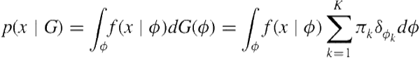
Mixture modeling is a probabilistic approach to model the existence of latent subpopulations in the data. A mixture component is represented by a cluster-specific⁴ probability density , where parametrizes the cluster distribution. For a data point , its subpopulation is assumed to be unknown thus the generative likelihood is modeled as a mixture from subpopulations:

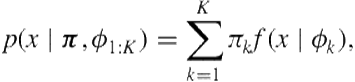(6.1)

where is the probability that belongs to the subpopulation and . This is the parametric and frequentist approach to mixture modeling. The expectation-maximization (EM) algorithm is typically employed to estimate the parameters and (s) from the data.

Under a Bayesian setting, the parameters and (s) are further endowed with prior distributions. Typically a symmetric Dirichlet distribution is used as the prior of , and the prior distributions for are model-specific depending on the form of the likelihood distribution . Conjugate priors are preferable; for example, if is a Bernoulli distribution, then conjugate prior distribution is a Beta distribution. Given the prior specification and defining as the density function for , Bayesian mixture models specify the generative likelihood for as:

(6.2)

Under this formalism, inference is required to derive the posterior distribution for and (s), which is often intractable. Markov Chain Monte Carlo methods, such as Gibbs sampling, are common approaches for the task. A latent indicator variable is introduced for each data point to specify its mixture component. Conditional on this latent variable, the distribution for is simplified to:

(6.3)

where . Full Gibbs sampling for posterior inference becomes straightforward by iteratively sampling the conditional distributions among the latent variable (s), and (s); that is,

(6.4)

(6.5)

(6.6)

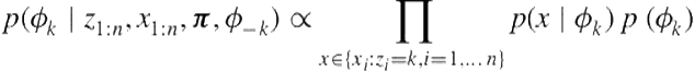
It is not difficult to recognize that the posterior for is again a Dirichlet, and with a conjugate prior, the posterior for also remains in the same form; thus, they are straightforward to sample.⁵ A collapsed Gibbs inference scheme can also be developed to improve the variance of the estimators by integrating out and (s), leaving out only the following conditional to sample from:

(6.7)

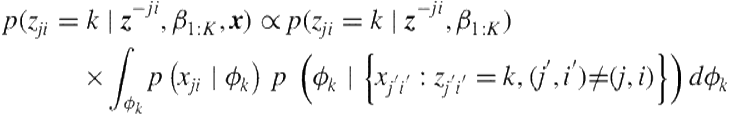
where is the number of assignments to cluster , excluding position , and is the hyperparameter for , assumed to be a symmetric Dirichlet distribution. The second term involves an integration that can easily be recognized as the predictive likelihood under a posterior distribution for . For conjugate prior, this expression can be analytically evaluated. Several results can readily be found in many standard Bayesian textbooks such as Gelman et al. [27].

A key theoretical limitation in the parametric Bayesian mixture model described so far is the assumption that the number of subpopulations in the data is known. In the realm of activity recognition, given the observed signals (s), each subpopulation can be interpreted as one class of activity, and it is desirable to infer the number of classes automatically. Model-selection methods such as cross-validation, Akaike information criterion (AIC), or Bayesian information criterion (BIC) can be used to estimate . However, these methods are still sensitive to held-out data. Moreover, it is expensive and difficult to reselect the model when new data arrives.

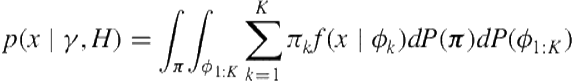
Recent advances in Bayesian nonparametric modeling provide a principled alternative to overcome these problems by introducing a nonparametric prior distribution on the parameters, thus allowing a countably infinite number of subpopulations, leading to aninfinite mixture formulation for data likelihood (compare to Eq. (6.1))

(6.8)

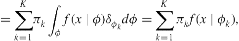
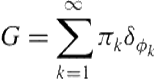
It is then natural to ask what would be a suitable prior distribution for infinite-dimensional objects that arise in the preceding equation. The answer to this is the Dirichlet process [23]. One way to motivate the arrival of the Bayesian nonparametric setting is to reconsider the mixture likelihood in Eq. (6.1). As usual, let , then construct a new discrete measure:

(6.9)

where denotes the atomic probability measure placing its mass at . The generative likelihood for data can be equivalently expressed as: where .

To see why, we express the conditional distribution for given as

(6.10)

(6.11)

which identically recovers the likelihood form in Eq. (6.1). Therefore, one sensible approach to move from a finite mixture representation in Eq. (6.1) to an infinite mixture in Eq. (6.8) is to define a discrete probability measure constructed from an infinite collection of atoms (s) sampled iid from the base measure and the weight (s):

(6.12)

Since both (s) and (s) are random, is also a random probability measure. It turns out that random discrete probability measures constructed in this way follow a Dirichlet process (DP).

Briefly, a Dirichlet process is a distribution over random probability measure on the parameter space and is specified by two parameters: is the concentration parameter and is base measure [23]. The terms “Dirichlet” and “base measure” come from the fact that for any finite partition of the measurable space , the random vector obtained by applying on this partition will distribute according to a Dirichlet distribution with parameters obtained from . Alternatively, the nonparametric object in Eq.(6.12) can be viewed as a limiting form of the parametric in Eq. (6.9) when and weights (s) are drawn from a symmetric Dirichlet [62]. Using as a nonparametric prior distribution, the data-generative process for infinite mixture models can be summarized as follows:

(6.13)

(6.14)

(6.15)

The representation for in Eq. (6.12) is known as the stick-breaking representation, taking the form , where and are the weights constructed through a stick-breaking process with [58]. It can be shown that with probability one, and we denote this process as . A recent book by Hjort et al. [29] provides an excellent account on theory and applications of DP.

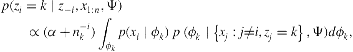
Inference in the DPM can be carried out under a Gibbs sampling scheme using the Polya urn characterization of the Dirichlet process [6]—also known as the Chinese restaurant process [54]. Again, let be the cluster indicator variable for , the collapsed Gibbs inference reduces to [43]:

(6.16)

where denotes the number of times the cluster has been used excluding position and is the predictive likelihood of observing under the mixture, which can be evaluated analytically thanks to the conjugacy between and . The expression in Eq. (6.16) illustrates the clustering property induced by DPM: a future data observation is more likely to return to an existing cluster with a probability proportional to its popularity ; however, it is also flexible enough to pick on a new value if needed as data grows beyond the complexity that the current model can explain. Furthermore, the number of clusters grow at under the Dirichlet process prior.

6.3.2 Hierarchical Dirichlet Process

Activity-recognition problems typically involve multiple sources of information either from an egocentric or device-centric point of view. In the former, the individual user acquires user-specific datasets, whereas in the later different sensors collect their own observations. Nonetheless, these data sources are often correlated by an underlying and hidden process that dictates how the data is observed. It is desirable to build a hierarchical model to learn activities from these multiple sources jointly by leveraging mutual statistical strength across datasets. This is known as the shrinkage effect in Bayesian analysis.

The Dirichlet process mixture model described in the previous section is suitable for analyzing a single data group, such as data that comes from an individual user or a single device. Moreover, the Dirichlet process can also be utilized as a nonparametric prior for modeling grouped data. Under this setting, each group is modeled as a DPM and these models are “linked” together to reflect the dependency among them.

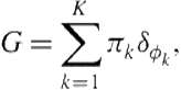
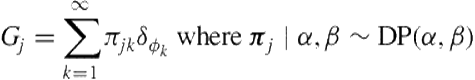
One particularly attractive formalism is the hierarchical Dirichlet process [61,62], which posits the dependency among the group-level DPM by another Dirichlet process. Due to the discreteness property of the DP, mixture components are naturally shared across groups. Specifically, let be the number of groups and be observations associated with the group , which are assumed to be exchangeable within the group. Under the HDP framework, each group is endowed with a random group-specific mixture distribution , which is hierarchically linked by another DP with a measure that itself is a draw from another DP:

(6.17)

(6.18)

The stick-breaking construction for HDP makes it clear how mixture components are shared across groups:

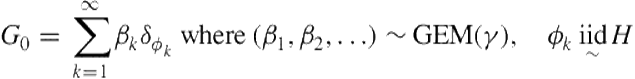(6.19)

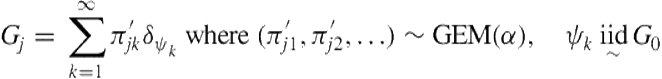(6.20)

Since is discrete, taking the support on , can equivalently be expressed [62] as:

(6.21)

Recall that and belong to the same mixture component if they are generated from the sample component parameter (i.e., ). Equations (6.19) and (6.21) immediately reveal that (s) share the same discrete support , thus mixture components are shared across groups.

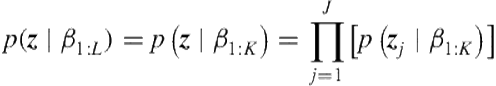
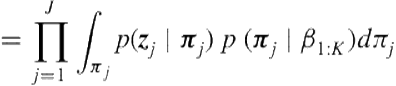
Integrating out the random measures (s) and , the posterior for (s) has been shown to follow a Chinese Restaurant Franchise process that can be used to develop an inference algorithm based on Gibbs sampling, and we refer to Teh et al. [62] for details. Alternatively, an auxiliary variable collapsed Gibbs sampling can be developed based on the stick-breaking representation by integrating out group-specific stick-breaking weights (s) and the atomic atoms (s) but explicitly sampling the stick weights (s) at the higher level as described in Teh et al. [62].

Assume is the number of clusters that have been created, but only components are active, which means the cluster indicator is limited within clusters . There are inactive components, which we shall cluster together and represent by . Therefore, using the additive property of Dirichlet distribution, can now be written as , where for and . Integrating out and (s) our Gibbs sampling state space is .

To sample , since there are only current active components, we can work out the conditional distribution for by discarding inactive components and integrating out within each group where we note that ; thus, we apply the marginal likelihood result for the Multinomial-Dirichlet conjugacy:

(6.22)

(6.23)

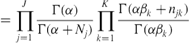(6.24)

With some further simple manipulations, we get . Therefore, together with the data (s), the Gibbs sampling equation for can be established:

(6.25)

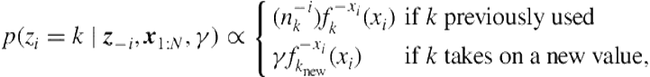
(6.26)

Again the last term is a form of predictive likelihood for under a standard Bayesian setting. It is model-specific but can be evaluated analytically when is conjugate to . Note that when resampling we have to consider the case that it may take on a new value . If introduces a new active cluster, we then need to update as follows: , , where , where the splitting step for and is justified by the splitting property of the Dirichlet distribution [62].

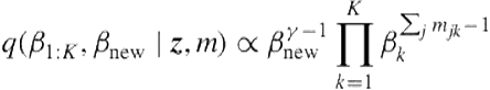
To sample , we express their conditional distribution, which turns out to be the ratio of two Gamma functions; therefore, as shown in Teh et al. [62], we sample them together with an auxiliary variable in which we note that conditional on follows a Dirichlet distribution:

(6.27)

(6.28)

The hyperparameters and can also be resampled by further endowing them with Gamma distributions and following the methods described in [22]. In this work, these hyperparameters are always resampled together with the main parameters. Lastly, assuming that the size of each group is roughly the same at , as shown in Teh and Jordan [61], the number of mixture components grows at , which is doubly logarithmically in and logarithmically in .

6.4 Experiments

Two datasets are used: the first collected in our lab using sociometric badges provided by Sociometric Solutions⁶ and the second is the well-known public Reality Mining data [20].

6.4.1 Sociometric Data

Sociometric badges were invented by the MIT Media Lab [47] and have been used in various applications. Figure 6.2 shows the front of a badge with the infrared sensor, the top-side microphone,⁷ and the programming mode button. These badges record a rich set of data, including anonymized speech features (e.g., volume, tone of voice, speaking time), body movement features derived from accelerometer sensors (e.g., energy and consistency), information of people nearby and face-to-face interaction with those who are also wearing a sociometric badge, the presence and signal strength of Bluetooth-enabled devices, and approximate location information. We briefly explain these features next.

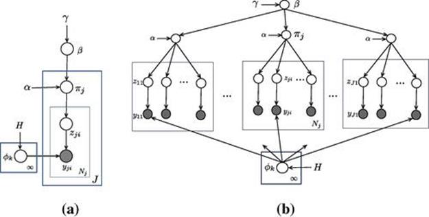
FIGURE 6.1 Generative model for Hierarchical Dirichlet Process. (a) Stick-breaking graphical model representation for HDP in plate notation. (b) Expanded graphical model representation over groups. Each box represents one group of data (e.g., document) with observed data points that are shaded. Unshaded nodes are latent variables. Each observed data point is assigned to a latent mixture indicator variable and are the concentration parameters and is the base measure. Each group of data possesses a separate mixture proportion vector of latent topics (s).

FIGURE 6.2 The front appearance of the sociometric badge (left) and its software user interface (right).

Body movement. Each badge has a three-axis accelerometer, set at a sampling rate of every 50 ms. For our data collection, a window frame of 10 s was used and the data were averaged within each window to construct one data point. We record the coordinate and two derived features: energy and consistency. Energy is simply the mean of three-axis signals , and the consistency attempts to capture the stability or consistency of the body movement computed as , where is the standard deviation of the values. These two features have been used in experiments previously with sociometric badges and are reported to be good features [45].

Proximity and people nearby. The badge has the capacity to record the opportunistic devices with Bluetooth enabled. It can detect the devices’ MAC addresses as well as the received signal strength indicators (RSSI).

We ordered 20 sociometric badges from Sociometric Solutions^TM, collecting data for three weeks on every working day, five days a week. However, due to some inconsistency in the way members of the lab were carrying and collecting data at the initial phase, we cleaned up and reported data from only 11 subjects in this chapter. We focus on two types of data here: accelerometer data and Bluetooth data. We refer to the accelerometer data as activity data and the Bluetooth data as colocation data.

6.4.1.1 Activity data

The sociometric badges record activity data from a three-axis accelerometer. We used the consistency measure [45] as the activity data representing the body movement. A consistency value closer to indicates less movement and closer to 0 if more movement was detected. We aim to extract basis latent activities from these signals, which might be used to build healthcare applications such as monitoring users with obesity or stress. Using Bayesian nonparametric approach, we treat each data point as a random draw from a univariate Gaussian with unknown mean and unknown precision :

(6.29)

Each Gaussian, parametrized by , represents one latent activity. We further specify the conjugate prior distribution for , which is a product of Gaussian-Gamma:

(6.30)

(6.31)

where , and are hyperparameters for the prior distribution in a standard Bayesian setting. These hyperparameters express the prior belief on the distribution of the parameter space and only need to be specified roughly [27]. A widely used approach is to carry out an empirical Bayes step using observed data to infer these parameters before running Gibbs. We adapt this strategy in this chapter.

For the activity data, values of a user on a day are grouped into a document, where each data point is the consistency value in a 10-second interval during the collection time. We run Gibbs sampling for 250 iterations with a burn-in period of 50 samples. The concentration parameters and are also resampled according to a Gamma distribution as described in Teh et al. [62]. Figure 6.3(a) plots the value for each Gibbs iteration, settling at around 1.2. Figure 6.3(b) shows the posterior distribution over the number of latent activities with a mode that is 4, and Figure 6.3(c) plots the estimated value of together with its mode as we run the Gibbs sampler. In this case, the model has inferred latent activity; each is represented by a univariate Gaussian distribution. These four activities are shown on the left side of Figure 6.4, which can be seen to be separated and captures the activity level well. The right side of Figure 6.4 illustrates an example of consistency signal from Subject 3 with his annotated activity.

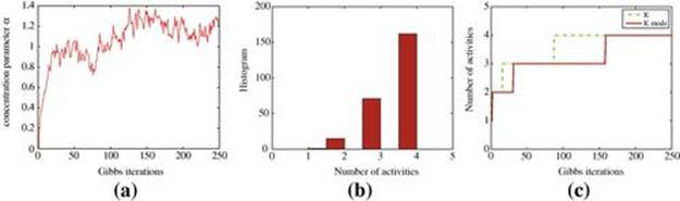
FIGURE 6.3 HDP results run for activity data acquired from sociometric badges from 11 subjects. (a) shows the concentration parameter being sampled at each Gibbs iteration, which tends to settle down around 1.2; (b) illustrates the empirical posterior distribution for the number of latent activities inferred; and (c) is a plot of the detailed value of and its mode tracked from the posterior distribution as Gibbs was run.

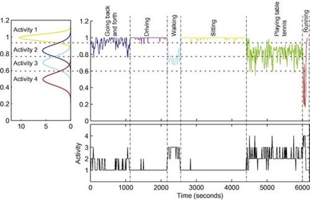
FIGURE 6.4 An illustration of accelerometer signals for different activity types. LHS: our model has learned four latent activities, each of which is represented by a univariate Gaussian: . -axis represents the consistency value derived from the accelerometer sensor described in Section 6.4.1. A learned latent activity implies a moving status of the subject. For example, Activity 1 has a mean close to 1, which represents the state of nonmovement (e.g., sitting). RHS: An example of consistency signal from Subject 3 with annotated activities. The decoded sequence of states is also plotted underneath. This decoded sequence was computed using the MAP estimation from the Gibbs samples; each state assumes a value in the set {1,2,3,4} corresponding to four latent activities discovered by HDP.

6.4.1.2 Colocation data

The sociometric badge regularly scans for surrounding Bluetooth devices including other badges. Therefore, we can derive the colocation information of the badge user. We used a window of 30 seconds to construct data in the form of count vectors. In each time interval, a data point is constructed for each user whose badge detects other badges. There are valid subjects in our sociometric dataset. Thus each data point is an 11-dimensional vector. With an element that represents the corresponding presence status of the subject, the owner of the data point is always present. Data from each day of a user is grouped into one document. All documents from all subjects are collected together to form a corpus to be used with the HDP (thus, each subject may correspond to multiple documents).

We model the observation probability as a multinomial distribution (the distribution in our description in Section 6.3.1) with a conjugate prior that is the Dirichlet (the base measure ). Thus, a latent colocation activity is described by a discrete distribution over the set satisfying and can be interpreted as follows: the higher probability of an entry represents the higher chance of its colocation with others. For example, and everywhere else indicate a strong colocation activity of Subjects 1 and 2.

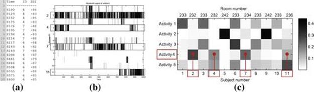
FIGURE 6.5 Illustration of Bluetooth raw signals, its representation and patterns extracted. (a) Examples of raw Bluetooth readings showing time of the event, user ID, and Bluetooth signal strengths. (b) An example of a Bluetooth data segment acquired for User 2 using the binary representation described in the text. (c) Five atomic latent colocation activities discovered by HDP, each of which is a multinomial distribution over 11 subjects (the darker, the higher probability (e.g., colocation Activity 4 shows the colocation of Subjects 2, 4, 7, and 11, as can also be seen visually in data from User 2)). Room number shows the actual room where each subject is sitting (e.g, user 11 sits in room 236).

Figure 6.6 plots various statistics from our Gibbs inference, which shows that our model has inferred five latent colocation activities from the data as shown in Figure 6.5. These activities are interpretable by inspecting against the ground truth from the lab. For example, the first activity represents the colocation of PhD students because they share the same room; the second captures only two subjects who happen to be two research fellows sharing the same room.

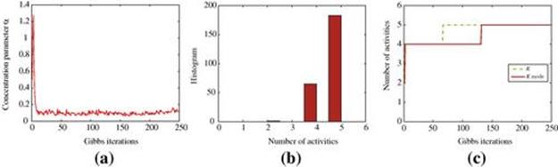
FIGURE 6.6 HDP results on colocation data collected from sociometric badges. (a) The concentration parameter , settling at around 0.2, (b) the posterior distribution on the number of latent activities, and (c) the estimated number of activity for each Gibbs and its mode tracked over time.

To further quantify the results from our model and demonstrate its strength over existing parametric models, we compare it to latent Dirichlet allocation [7], which has been used regularly as the state-of-the-art method for activity profiling and modeling in pervasive settings [30,51,53]. For each subject, we derive an average mixture proportion of latent activities (topics) from (s) vectors learned from the data for that subject. We then use Jensen-Shannon divergence to compute the distance between each pair of subjects. The Jensen-Shannon divergence for two discrete distribution and is defined as:

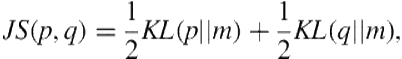(6.32)

where and is the Kullback-Leibler divergence. The similarity between two subjects and is then defined as:

(6.33)

where, with a little abuse of notation, and are the average mixture proportion for Subjects and , respectively.

Figure 6.7 represents the similarity matrix obtained from the HDP, which automatically infers the number of activities, and the LDA, which prespecifies the number of activities to 5. Visual inspection shows a clear separation in the result from the HDP compared to LDA.

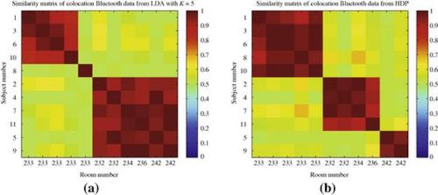
FIGURE 6.7 Similarity matrix obtained for 11 subjects using colocation Bluetooth data from sociometric badge dataset. (a) Using LDA for five activities and (b) using HDP. Similarity is computed for each pair of users using the Jensen-Shannon divergence between mixture proportions of activities being used by the two subjects.

To further substantiate and understand the proposed framework, we run LDA for various predefined values of and construct a gross ground truth by dividing 11 subjects into four groups according to the room they share: the first includes 5 PhD students and the next 6 users are divided into 3 groups (2 subjects in one room, except Subjects 7 and 11, who are in two adjacent rooms). We then use the Affinity Propagation (AP) algorithm [25] to perform a clustering. AP uses the similarity matrix as input and Figure 6.8reports the clustering results using popular performance metrics in clustering and data mining literature, which includes F-measure, cluster purity, Rand index, and normalized mutual information (NMI); further details can be found in Jiawei and Kamber [32] and Manning et al. [41]. As can be clearly seen, HDP achieves the best result without the need for specifying the number of activities (topics) in advance, whereas LDA results are sensitive and dictated by this model specification. HDP has achieved a reasonably high performance: an F-measure and a NMI close to 0.9 and Rand index of more than 0.9.

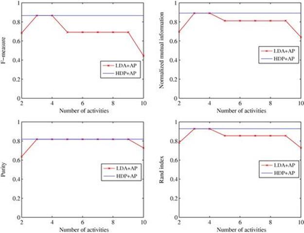
FIGURE 6.8 Performance of LDA + AP and HDP + AP on colocation data. Since HDP automatically learns the number of activities (5 in this case), we repeat this result for HDP over the horizontal axis for easy comparison with LDA.

6.4.2 Reality Mining Data

Reality Mining [20] is a well-known mobile phone dataset collected at the MIT Media Lab involving 100 users over 9 months; a wide range of information from each phone was recorded (see appendix of Lambert [37] for a full description of the database schema). To demonstrate the feasibility of our proposed framework, we focus on the Bluetooth events. Using Bluetooth-recoded events as colocation information, our goal is to automatically learn activity of subject colocation in this dataset.

Using this information, we further compute the similarity between subjects and group them into clusters. The affiliation information recorded in the database is used as the ground truth in which subjects can be roughly divided into labeled groups (e.g., staff, master frosh, professor, Sloan Business School students). Removing groups of less than 2 members and users whose affiliations are missing, we ended up with a total of subjects divided into 8 groups in our dataset. For each subject, we construct 1 data point for every 10 minutes of recording. Each data point is a 69-dimensional vector with an element that is set to 1 if the corresponding subject is present and 0 otherwise (self-presence is always set to 1). All data points for each subject are treated as one collection of data, analogous to a document or a group in our HDP description.

Similar to colocation data from sociometric badges, each latent topic is a multinomial distribution over the set of users . In this case, nine activities have been discovered and visualized in Table 6.1. Visual inspection reveals some interesting activities: Activity 3, for example, shows a strong colocation of only Subjects 21 and 40; Activity 9 shows that Subject 55 mostly works alone; Activity 2 shows a typical colocation of Sloan Business School students; and so on.

Table 6.1

Visualization for Nine Latent Activities Learned by HDP

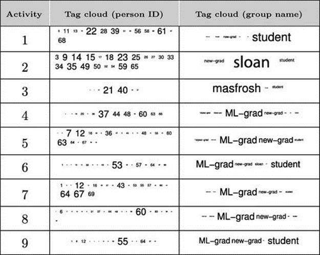
Note: Each is a discrete distribution over the set of V 69 subjects in the Reality Mining data. Each number corresponds to an index of a subject and its size is proportional to the probability within that activity. The tag cloud column visualizes the tag cloud of affiliation labels for each activity.

Figure 6.9 attempts to construct a clustering structure directly by using the mixture probability of latent activities assigned for each user. This colocation network is generated by thresholding the (topic, user) mixture matrix learned from HDP. The resultant matrix is then used as the adjacency matrix. In this network, the Sloan Business School students and the master frosh students are usually colocated with other members of the same group. On the other hand, members of the Media Lab might be colocated with members of other affiliation groups.

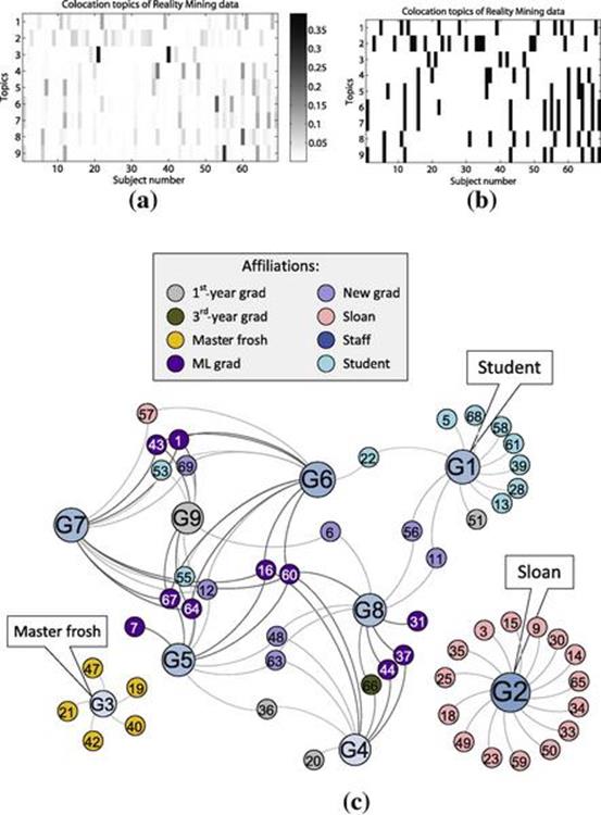
FIGURE 6.9 A clustering structure constructed using the mixture probability of latent activities. (a) The matrix represents the probability of latent activities (topics) given subjects (69 from Reality Mining data) and (b) after applying a hard-threshold to convert it to a binary adjacency matrix. (c) Graphic visualization based on adjacency matrix inferred from latent activities with the node colors representing the affiliation labels from the ground truth.

To further demonstrate the strength of the Bayesian nonparametric approach, we again perform a clustering experiment similar to the setting reported for colocation data in the Colocation data section and compared against LDA. We use the mixture proportion of activity and Jensen-Shannon divergence to compute the distance between users and similarity measures in Eq. (6.33). Figure 6.10 shows the similarity matrix for Reality Mining data. It can be clearly seen that Sloan Business School students and master frosh students are in two separate groups. This is because the Sloan students are physically adjacent to the Media Lab, while master frosh students only join the lab at particular times. Table 6.2 shows ground truth groups in Reality Mining data and Table 6.3 presents the clustering result using HDP and AP. Figure 6.11 further shows the performance comparison of HDP against LDA (run for various values of ). Again HDP consistently delivers a performance comparable to the best performance of LDA, which requires searching over the parameter space.

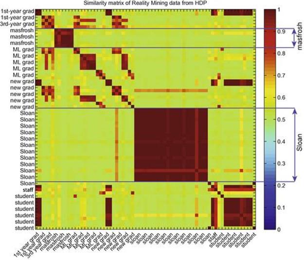
FIGURE 6.10 Similarity matrix for 69 subjects from Reality Mining data using the results from HDP.

Table 6.2

Eight Ground Truth Groups in Reality Mining Data

Table 6.3

Clustering Result Data Using HDP + AP

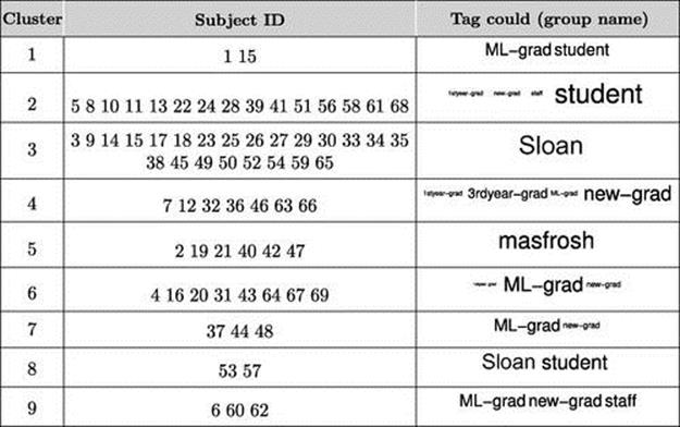
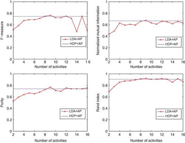
FIGURE 6.11 Performance of LDA + AP and HDP + AP on Reality Mining data.

6.5 Conclusion

Learning latent activities that are nontrivially present in the raw sensor data is important to many activity-aware applications, and this chapter has explored the use of Bayesian nonparametric models for this task. In particular, we make use of the hierarchical Dirichlet process to discover movement and colocation activities from social signals. The key advantage of this approach is its ability to learn the number of latent activities automatically and grow with the data, thus completely bypassing the fundamental difficulty of model selection encountered in parametric models. We use data collected by sociometric badges in the lab as well as the public Reality Mining dataset. In all cases, we have demonstrated how the framework can be used, illustrated insights in the activities discovered, and used them for clustering tasks. To demonstrate the strengths and key advantages of the framework, we have rigorously compared the performance against state-of-the-art existing models and demonstrated that high performance is consistently achieved.

References

1. Abowd GD, Mynatt ED. Charting past, present, and future: research in ubiquitous computing. ACM Trans Comput Human Interact. 2000;7(1):29-58.

2. Bao L, Intille SS. Activity recognition from user-annotated acceleration data. In: Lecture notes in computer science; 2004. p. 1–17.

3. Bargh MS, de Groote R. Indoor localization based on response rate of Bluetooth inquiries. In: Proceedings of the First ACM International Workshop on Mobile Entity Localization and Tracking in GPS-less Environments; 2008. p. 49–54.

4. Bellos C, Papadopoulos A, Rosso R, Fotiadis DI. Heterogeneous data fusion and intelligent techniques embedded in a mobile application for real-time chronic disease management. Engineering in Medicine and Biology Society, Annual International Conference of the IEEE. 2011:8303-8306.

5. Bettini C, Brdiczka O, Henricksen K, Indulska J, Nicklas D, Ranganathan A, et al. A survey of context modeling and reasoning techniques. Pervasive Mobile Comput. 2010;6(2):161-180.

6. Blackwell D, MacQueen JB. Ferguson distributions via Pólya urn schemes. Ann Stat. 1973;1(2):353-355.

7. Blei DM, Ng AY, Jordan MI. Latent Dirichlet allocation. J Mach Learn Res. 2003;3:993-1022.

8. Boston D, Mardenfeld S, Susan Pan J, Jones Q, Iamnitchi A, Borcea C. Leveraging Bluetooth co-location traces in group discovery algorithms. Pervasive Mobile Comput. 2012. doi:10.1016/j.pmcj.2012.10.003.

9. Bui H, Phung D, Venkatesh S, Phan H. The hidden permutation model and location-based activity recognition. Proceedings of the National Conference on Artificial Intelligence. July 2008:1345-1350.

10. Burns A, Greene BR, McGrath MJ, O’Shea TJ, Kuris B, Ayer SM, et al. SHIMMER^TM—a wireless sensor platform for noninvasive biomedical research. IEEE Sens J. 2010;10(9):1527-1534.

11. Chellappa R, Vaswani N, Chowdhury AKR. Activity modeling and recognition using shape theory. In: Behavior representation in modeling and simulation; 2003. p. 151–4.

12. Choudhury T, Consolvo S, Harrison B, Hightower J, LaMarca A, LeGrand L, et al. The mobile sensing platform: an embedded activity recognition system. Pervasive Comput IEEE. 2008;7(2):32-41.

13. Del Din S, Patel S, Cobelli C, Bonato P. Estimating Fugl-Meyer clinical scores in stroke survivors using wearable sensors. Engineering in Medicine and Biology Society, Annual International Conference of the IEEE. 2011:5839-5842.

14. Della Toffola L, Patel S, Chen B, Ozsecen YM, Puiatti A, Bonato P. Development of a platform to combine sensor networks and home robots to improve fall detection in the home environment. Engineering in Medicine and Biology Society, Annual International Conference of the IEEE. 2011:5331-5334.

15. Derényi I, Palla G, Vicsek T. Clique percolation in random networks. Phys Rev Lett. 2005;94(16):160202.

16. Dey AK. Understanding and using context. Personal Ubiquitous Comput. 2001;5(1):4-7.

17. Dong W, Lepri B, Pentland AS. Modeling the co-evolution of behaviors and social relationships using mobile phone data. Proceedings of the Tenth International Conference on Mobile and Ubiquitous Multimedia. 2011:134-143.

18. Duong T, Phung D, Bui H, Venkatesh S. Human behavior recognition with generic exponential family duration modeling in the hidden semi-Markov model. International Conference on Pattern Recognition. vol. 3. 2006:202-207.

19. Duong T, Phung D, Bui H, Venkatesh S. Efficient duration and hierarchical modeling for human activity recognition. Artif Intell. 2009;173(7–8):830-856.

20. Eagle N, Pentland A. Reality mining: sensing complex social systems. Personal Ubiquitous Comput. 2006;10(4):255-268.

21. Eagle N, Pentland AS. Eigenbehaviors: identifying structure in routine. Behav Ecol Sociobiol. 2009;63(7):1057-1066.

22. Escobar MD, West M. Bayesian density estimation and inference using mixtures. J Am Stat Assoc. 1995;90(430):577-588.

23. Ferguson TS. A Bayesian analysis of some nonparametric problems. Ann Stat. 1973;1(2):209-230.

24. Fortune E, Tierney M, Scanaill CN, Bourke A, Kennedy N, Nelson J. Activity level classification algorithm using SHIMMER^TM wearable sensors for individuals with rheumatoid arthritis. Annual International Conference of the IEEE Engineering in Medicine and Biology Society. 2011:3059-3062.

25. Frey BJ, Dueck D. Clustering by passing messages between data points. Science. 2007;315:972-976.

26. Gaggioli A, Pioggia G, Tartarisco G, Baldus G, Corda D, Cipresso P, et al. A mobile data collection platform for mental health research. Personal Ubiquitous Comput. 2013;17(2):241-251.

27. Gelman A, Carlin JB, Stern HS, Rubin DB. Bayesian data analysis. Chapman & Hall/CRC; 2003.

28. Hay S, Harle R. Bluetooth tracking without discoverability. Location and context awareness. Springer; 2009:120-137.

29. Hjort NL, Holmes C, Müller P, Walker SG. Bayesian nonparametrics. Cambridge University Press; 2010.

30. Huynh T, Fritz M, Schiele B. Discovery of activity patterns using topic models. Proceedings of the Tenth International Conference on Ubiquitous Computing. 2008:10-19.

31. Huynh T, Schiele Bv. Unsupervised discovery of structure in activity data using multiple eigenspaces. In: Hazas M, Krumm J, Strang T, eds. Location and context awareness. Springer; 2006:151-167.

32. Jiawei H, Kamber M. Data mining: concepts and techniques. Morgan Kaufmann; 2001.

33. Kim S, Li M, Lee S, Mitra U, Emken A, Spruijt-Metz D, et al. Modeling high-level descriptions of real-life physical activities using latent topic modeling of multimodal sensor signals. Engineering in Medicine and Biology Society, Annual International Conference of the IEEE. 2011:6033-6036.

34. Kondragunta J. Building a context aware infrastructure using Bluetooth. PhD thesis, University of California, Irvine; 2009.

35. Kumpula JM, Kivelä M, Kaski K, Saramäki J. Sequential algorithm for fast clique percolation. Phys Rev E. 2008;78(2):026109.

36. Kwapisz JR, Weiss GM, Moore SA. Activity recognition using cell phone accelerometers. ACM SIGKDD Exploration Newsl. 2011;12(2):74-82.

37. Lambert MJ. Visualizing and analyzing human-centered data streams. PhD thesis, Massachusetts Institute of Technology; 2005.

38. Lorincz K, Chen B, Challen GW, Chowdhury AR, Patel S, Bonato P, et al. Mercury: a wearable sensor network platform for high-fidelity motionanalysis. Proceedings of the Seventh ACM Conference on Embedded Networked Sensor Systems. 2009:183-196.

39. Lu H, Frauendorfer D, Rabbi M, Schmid Mast M, Chittaranjan GT, Campbell AT, et al. StressSense: detecting stress in unconstrained acoustic environments using smartphones. Proceedings of the ACM Conference on Ubiquitous Computing. 2012:351-360.

40. Lu H, Yang J, Liu Z, Lane ND, Choudhury T, Campbell AT. The jigsaw continuous sensing engine for mobile phone applications. Proceedings of the Eighth ACM Conference on Embedded Networked Sensor Systems. 2010:71-84.

41. Manning CD, Raghavan P, Schütze H. Introduction to information retrieval. vol. 1. Cambridge University Press; 2008.

42. Mardenfeld S, Boston D, Juan Pan S, Jones Q, Iamntichi A, Borcea C. GDC: group discovery using co-location traces. IEEE Second International Conference on Social Computing. 2010:641-648.

43. Neal RM. Markov chain sampling methods for Dirichlet process mixture models. J Comput Graphical Stat. 2000;9:249-265.

44. Nicolai T, Kenn H. Towards detecting social situations with Bluetooth. In: Adjunct Proceedings Ubicomp; 2006.

45. Olguín DO. Sociometric badges: wearable technology for measuring human behavior. PhD thesis, Massachusetts Institute of Technology; 2007.

46. Olguín DO, Pentland AS. Human activity recognition: accuracy across common locations for wearable sensors. Citeseer; 2006.

47. Olguín DO, Pentland AS. Social sensors for automatic data collection. In: Americas conference on information systems; 2008. p. 171.

48. Padasdao B, Boric-Lubecke O. Respiratory rate detection using a wearable electromagnetic generator. Engineering in Medicine and Biology Society, EMBC, 2011 Annual International Conference of the IEEE. 2011:3217-3220.

49. Palla G, Derényi I, Farkas I, Vicsek T. Uncovering the overlapping community structure of complex networks in nature and society. Nature. 2005;435(7043):814-818.

50. Pentland AS. Honest signals: how they shape our world. The MIT Press; 2008.

51. Phung D, Adams B, Tran K, Venkatesh S, Kumar M. High accuracy context recovery using clustering mechanisms. Proceedings of the IEEE International Conference on Pervasive Computing and Communications. March 2009:1-9.

52. Phung D, Adams B, Venkatesh S. Computable social patterns from sparse sensor data. In: First international workshop on location and the web, in conjuntion with the world wide web conference; 2008. p. 69–72.

53. Phung D, Adams B, Venkatesh S, Kumar M. Unsupervised context detection using wireless signals. Pervasive Mobile Comput. 2009;5(6):714-733.

54. Pitman J. Combinatorial stochastic processes. Lecture notes in mathematics. vol. 1875. Springer-Verlag; 2006:7-24 [Lectures from the 32nd summer school on probability theory, Saint-Flour, 2002, with a foreword by Jean Picard].

55. Puiatti A, Mudda S, Giordano S, Mayora O. Smartphone-centred wearable sensors network for monitoring patients with bipolar disorder. Engineering in Medicine and Biology Society, Annual International Conference of the IEEE. 2011:3644-3647.

56. Rashidi P. Stream sequence mining for human activity discovery. In: Sukthankar G, Goldman RP, Geib C, Pynadath DV, Bui HH, eds. Plan, activity, and intent recognition. Waltham, MA: Morgan Kaufmann Publishers; 2014:123-148.

57. Ravi N, Dandekar N, Mysore P, Littman ML. Activity recognition from accelerometer data. Proceedings of the National Conference on Artificial Intelligence. vol. 20. 2005:1541-1546.

58. Sethuraman J. A constructive definition of Dirichlet priors. Statistica Sinica. 1994;4(2):639-650.

59. Munguia Tapia E. Activity recognition in the home setting using simple and ubiquitous sensors. PhD thesis, Massachusetts Institute of Technology; 2003.

60. Tasoulis SK, Doukas CN, Maglogiannis I, Plagianakos VP. Statistical data mining of streaming motion data for fall detection in assistive environments. Engineering in Medicine and Biology Society, Annual International Conference of the IEEE. 2011:3720-3723.

61. Teh YW, Jordan MI. Hierarchical Bayesian nonparametric models with applications. In: Hjort N, Holmes C, Müller P, Walker S, eds. Bayesian nonparametrics: principles and practice. Cambridge University Press; 2009:158.

62. Teh YW, Jordan MI, Beal MJ, Blei DM. Hierarchical Dirichlet processes. J Am Stat Assoc. 2006;101(476):1566-1581.

63. Tolkiehn M, Atallah L, Lo B, Yang GZ. Direction sensitive fall detection using a triaxial accelerometer and a barometric pressure sensor. Engineering in Medicine and Biology Society, Annual International Conference of the IEEE. 2011:369-372.

64. Valtonen M, Maentausta J, Vanhala J. Tiletrack: capacitive human tracking using floor tiles. IEEE International Conference on Pervasive Computing and Communications. 2009:1-10.

65. Valtonen M, Vanhala J. Human tracking using electric fields. IEEE International Conference on Pervasive Computing and Communications. 2009:1-3.

66. Wang L, Suter D. Recognizing human activities from silhouettes: motion subspace and factorial discriminative graphical model. IEEE Conference on Computer Vision and Pattern Recognition. 2007:1-8.

67. Zhang Z, Kapoor U, Narayanan M, Lovell NH, Redmond SJ. Design of an unobtrusive wireless sensor network for nighttime falls detection. Engineering in Medicine and Biology Society, International Conference of the IEEE. 2011:5275-5278.

68. Zheng H, Wang H, Black N. Human activity detection in smart home environment with self-adaptive neural networks. IEEE International Conference on Networking, Sensing and Control. 2008:1505-1510.