Computer Organization and Design (2016)
Parallel Processors from Client to Cloud
This chapter explains how computer architects have long sought to create powerful computers simply by connecting many existing smaller ones. It shows that multiprocessor software must be designed to work with a variable number of processors. One consequence of this is that energy has become the overriding issue for both microprocessors and datacenters. Replacing large inefficient processors with many smaller, efficient processors can deliver better performance per joule both in the large and in the small, but only if software can efficiently use them. Improved energy efficiency joins scalable performance in making the case for the use of multiprocessors. This parallel revolution in the hardware/software interface is perhaps the greatest challenge facing the field. The chapter explains that this revolution will provide many new research and business prospects inside and outside the IT field, and the companies that dominate the multicore era may not be the same ones that dominated the uniprocessor era. It emphasizes that understanding the underlying hardware trends and learning to adapt software to them is where innovation and technical advances will occur in the years ahead.
Keywords
multicore; uniprocessor; parallel; parallelism; parallel processing programs; multiprocessor; uniprocessor; shared memory multiprocessors; cluster; clusters; message-passing; message-passing multiprocessors; hardware multithreading; Single Instruction stream; SISD; Multiple Instruction streams; MIMD; Single Instruction streams Multiple Data streams; SIMD; Single Program Multiple Data; SPMD; Vector; graphics processing unit; GPU; multiprocessor network topology; Roofline model; job-level parallelism; process-level parallelism; multicore microprocessor; core; strong scaling; weak scaling; shared memory multiprocessor; SMP; uniform memory access; UMA; nonuniform memory access; NUMA; synchronization; lock; reduction; message passing; send message routine; receive message routine; hardware multithreading; fine-grained multithreading; coarse-grained multithreading; simultaneous multithreading; SMT; data-level parallelism; network bandwidth; bisection bandwidth; fully connected network; multistage network; fully connected network; crossbar network; Pthreads; OpenMP; arithmetic intensity; software as a service; Cloud Computing; Warehouse Scale Computer; WSC; NVIDIA; GPU computing
“I swing big, with everything I’ve got. I hit big or I miss big. I like to live as big as I can.”
Babe Ruth American baseball player
6.1 Introduction
6.2 The Difficulty of Creating Parallel Processing Programs
6.3 SISD, MIMD, SIMD, SPMD, and Vector
6.4 Hardware Multithreading
6.5 Multicore and Other Shared Memory Multiprocessors
6.6 Introduction to Graphics Processing Units
6.7 Clusters, Warehouse Scale Computers, and Other Message-Passing Multiprocessors
6.8 Introduction to Multiprocessor Network Topologies
![]() 6.9 Communicating to the Outside World: Cluster Networking
6.9 Communicating to the Outside World: Cluster Networking
6.10 Multiprocessor Benchmarks and Performance Models
6.11 Real Stuff: Benchmarking Intel Core i7 versus NVIDIA Tesla GPU
6.12 Going Faster: Multiple Processors and Matrix Multiply
6.13 Fallacies and Pitfalls
6.14 Concluding Remarks
![]() 6.15 Historical Perspective and Further Reading
6.15 Historical Perspective and Further Reading
6.16 Exercises
Multiprocessor or Cluster Organization
6.1 Introduction
Over the Mountains Of the Moon, Down the Valley of the Shadow, Ride, boldly ride the shade replied—If you seek for El Dorado!
Edgar Allan Poe, “El Dorado,” stanza 4, 1849
Computer architects have long sought the “The City of Gold” (El Dorado) of computer design: to create powerful computers simply by connecting many existing smaller ones. This golden vision is the fountainhead of multiprocessors. Ideally, customers order as many processors as they can afford and receive a commensurate amount of performance. Thus, multiprocessor software must be designed to work with a variable number of processors. As mentioned in Chapter 1, energy has become the overriding issue for both microprocessors and datacenters. Replacing large inefficient processors with many smaller, efficient processors can deliver better performance per joule both in the large and in the small, if software can efficiently use them. Thus, improved energy efficiency joins scalable performance in the case for multiprocessors.
multiprocessor
A computer system with at least two processors. This computer is in contrast to a uniprocessor, which has one, and is increasingly hard to find today.
Since multiprocessor software should scale, some designs support operation in the presence of broken hardware; that is, if a single processor fails in a multiprocessor with n processors, these system would continue to provide service with n−1 processors. Hence, multiprocessors can also improve availability (see Chapter 5).
High performance can mean high throughput for independent tasks, called task-level parallelism or process-level parallelism. These tasks are independent single-threaded applications, and they are an important and popular use of multiple processors. This approach is in contrast to running a single job on multiple processors. We use the term parallel processing program to refer to a single program that runs on multiple processors simultaneously.

task-level parallelism or process-level parallelism
Utilizing multiple processors by running independent programs simultaneously.
parallel processing program
A single program that runs on multiple processors simultaneously.
There have long been scientific problems that have needed much faster computers, and this class of problems has been used to justify many novel parallel computers over the decades. Some of these problems can be handled simply today, using a cluster composed of microprocessors housed in many independent servers (see Section 6.7). In addition, clusters can serve equally demanding applications outside the sciences, such as search engines, Web servers, email servers, and databases.
cluster
A set of computers connected over a local area network that function as a single large multiprocessor.
As described in Chapter 1, multiprocessors have been shoved into the spotlight because the energy problem means that future increases in performance will primarily come from explicit hardware parallelism rather than much higher clock rates or vastly improved CPI. As we said in Chapter 1, they are called multicore microprocessors instead of multiprocessor microprocessors, presumably to avoid redundancy in naming. Hence, processors are often called cores in a multicore chip. The number of cores is expected to increase with Moore’s Law. These multicores are almost always Shared Memory Processors (SMPs), as they usually share a single physical address space. We’ll see SMPs more in Section 6.5.

multicore microprocessor
A microprocessor containing multiple processors (“cores”) in a single integrated circuit. Virtually all microprocessors today in desktops and servers are multicore.
shared memory multiprocessor (SMP)
A parallel processor with a single physical address space.
The state of technology today means that programmers who care about performance must become parallel programmers, for sequential code now means slow code.
The tall challenge facing the industry is to create hardware and software that will make it easy to write correct parallel processing programs that will execute efficiently in performance and energy as the number of cores per chip scales.
This abrupt shift in microprocessor design caught many off guard, so there is a great deal of confusion about the terminology and what it means. Figure 6.1 tries to clarify the terms serial, parallel, sequential, and concurrent. The columns of this figure represent the software, which is either inherently sequential or concurrent. The rows of the figure represent the hardware, which is either serial or parallel. For example, the programmers of compilers think of them as sequential programs: the steps include parsing, code generation, optimization, and so on. In contrast, the programmers of operating systems normally think of them as concurrent programs: cooperating processes handling I/O events due to independent jobs running on a computer.
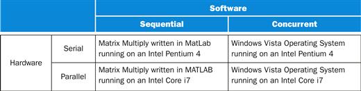
FIGURE 6.1 Hardware/software categorization and examples of application perspective on concurrency versus hardware perspective on parallelism.
The point of these two axes of Figure 6.1 is that concurrent software can run on serial hardware, such as operating systems for the Intel Pentium 4 uniprocessor, or on parallel hardware, such as an OS on the more recent Intel Core i7. The same is true for sequential software. For example, the MATLAB programmer writes a matrix multiply thinking about it sequentially, but it could run serially on the Pentium 4 or in parallel on the Intel Core i7.
You might guess that the only challenge of the parallel revolution is figuring out how to make naturally sequential software have high performance on parallel hardware, but it is also to make concurrent programs have high performance on multiprocessors as the number of processors increases. With this distinction made, in the rest of this chapter we will use parallel processing program or parallel software to mean either sequential or concurrent software running on parallel hardware. The next section of this chapter describes why it is hard to create efficient parallel processing programs.
Before proceeding further down the path to parallelism, don’t forget our initial incursions from the earlier chapters:
■ Chapter 2, Section 2.11: Parallelism and Instructions: Synchronization
■ Chapter 3, Section 3.6: Parallelism and Computer Arithmetic: Subword Parallelism
■ Chapter 4, Section 4.10: Parallelism via Instructions
■ Chapter 5, Section 5.10: Parallelism and Memory Hierarchy: Cache Coherence
Check Yourself
True or false: To benefit from a multiprocessor, an application must be concurrent.
6.2 The Difficulty of Creating Parallel Processing Programs
The difficulty with parallelism is not the hardware; it is that too few important application programs have been rewritten to complete tasks sooner on multiprocessors. It is difficult to write software that uses multiple processors to complete one task faster, and the problem gets worse as the number of processors increases.
Why has this been so? Why have parallel processing programs been so much harder to develop than sequential programs?
The first reason is that you must get better performance or better energy efficiency from a parallel processing program on a multiprocessor; otherwise, you would just use a sequential program on a uniprocessor, as sequential programming is simpler. In fact, uniprocessor design techniques such as superscalar and out-of-order execution take advantage of instruction-level parallelism (see Chapter 4), normally without the involvement of the programmer. Such innovations reduced the demand for rewriting programs for multiprocessors, since programmers could do nothing and yet their sequential programs would run faster on new computers.
Why is it difficult to write parallel processing programs that are fast, especially as the number of processors increases? In Chapter 1, we used the analogy of eight reporters trying to write a single story in hopes of doing the work eight times faster. To succeed, the task must be broken into eight equal-sized pieces, because otherwise some reporters would be idle while waiting for the ones with larger pieces to finish. Another speedup obstacle could be that the reporters would spend too much time communicating with each other instead of writing their pieces of the story. For both this analogy and parallel programming, the challenges include scheduling, partitioning the work into parallel pieces, balancing the load evenly between the workers, time to synchronize, and overhead for communication between the parties. The challenge is stiffer with the more reporters for a newspaper story and with the more processors for parallel programming.
Our discussion in Chapter 1 reveals another obstacle, namely Amdahl’s Law. It reminds us that even small parts of a program must be parallelized if the program is to make good use of many cores.
Speedup Challenge
Example
Suppose you want to achieve a speedup of 90 times faster with 100 processors. What percentage of the original computation can be sequential?
Answer
Amdahl’s Law (Chapter 1) says
![]()
We can reformulate Amdahl’s Law in terms of speedup versus the original execution time:

This formula is usually rewritten assuming that the execution time before is 1 for some unit of time, and the execution time affected by improvement is considered the fraction of the original execution time:
Substituting 90 for speedup and 100 for amount of improvement into the formula above:
Then simplifying the formula and solving for fraction time affected:
Thus, to achieve a speedup of 90 from 100 processors, the sequential percentage can only be 0.1%.
Yet, there are applications with plenty of parallelism, as we shall see next.
Speedup Challenge
Bigger Problem
Example
Suppose you want to perform two sums: one is a sum of 10 scalar variables, and one is a matrix sum of a pair of two-dimensional arrays, with dimensions 10 by 10. For now let’s assume only the matrix sum is parallelizable; we’ll see soon how to parallelize scalar sums. What speedup do you get with 10 versus 40 processors? Next, calculate the speedups assuming the matrices grow to 20 by 20.
Answer
If we assume performance is a function of the time for an addition, t, then there are 10 additions that do not benefit from parallel processors and 100 additions that do. If the time for a single processor is 110 t, the execution time for 10 processors is
![]()
![]()
so the speedup with 10 processors is 110t/20t=5.5. The execution time for 40 processors is
![]()
so the speedup with 40 processors is 110t/12.5t=8.8. Thus, for this problem size, we get about 55% of the potential speedup with 10 processors, but only 22% with 40.
Look what happens when we increase the matrix. The sequential program now takes 10t+400t=410t. The execution time for 10 processors is
![]()
so the speedup with 10 processors is 410t/50t=8.2. The execution time for 40 processors is
![]()
so the speedup with 40 processors is 410t/20t=20.5. Thus, for this larger problem size, we get 82% of the potential speedup with 10 processors and 51% with 40.
These examples show that getting good speedup on a multiprocessor while keeping the problem size fixed is harder than getting good speedup by increasing the size of the problem. This insight allows us to introduce two terms that describe ways to scale up.
Strong scaling means measuring speedup while keeping the problem size fixed. Weak scaling means that the problem size grows proportionally to the increase in the number of processors. Let’s assume that the size of the problem, M, is the working set in main memory, and we have P processors. Then the memory per processor for strong scaling is approximately M/P, and for weak scaling, it is approximately M.
strong scaling
Speedup achieved on a multiprocessor without increasing the size of the problem.
weak scaling
Speedup achieved on a multiprocessor while increasing the size of the problem proportionally to the increase in the number of processors.
Note that the memory hierarchy can interfere with the conventional wisdom about weak scaling being easier than strong scaling. For example, if the weakly scaled dataset no longer fits in the last level cache of a multicore microprocessor, the resulting performance could be much worse than by using strong scaling.

Depending on the application, you can argue for either scaling approach. For example, the TPC-C debit-credit database benchmark requires that you scale up the number of customer accounts in proportion to the higher transactions per minute. The argument is that it’s nonsensical to think that a given customer base is suddenly going to start using ATMs 100 times a day just because the bank gets a faster computer. Instead, if you’re going to demonstrate a system that can perform 100 times the numbers of transactions per minute, you should run the experiment with 100 times as many customers. Bigger problems often need more data, which is an argument for weak scaling.
This final example shows the importance of load balancing.
Speedup Challenge
Balancing Load
Example
To achieve the speedup of 20.5 on the previous larger problem with 40 processors, we assumed the load was perfectly balanced. That is, each of the 40 processors had 2.5% of the work to do. Instead, show the impact on speedup if one processor’s load is higher than all the rest. Calculate at twice the load (5%) and five times the load (12.5%) for that hardest working processor. How well utilized are the rest of the processors?
Answer
If one processor has 5% of the parallel load, then it must do 5%×400 or 20 additions, and the other 39 will share the remaining 380. Since they are operating simultaneously, we can just calculate the execution time as a maximum
![]()
The speedup drops from 20.5 to 410t/30t=14. The remaining 39 processors are utilized less than half the time: while waiting 20t for hardest working processor to finish, they only compute for 380t/39=9.7t.
If one processor has 12.5% of the load, it must perform 50 additions. The formula is:
![]()
The speedup drops even further to 410t/60t=7. The rest of the processors are utilized less than 20% of the time (9t/50t). This example demonstrates the importance of balancing load, for just a single processor with twice the load of the others cuts speedup by a third, and five times the load on just one processor reduces speedup by almost a factor of three.
Now that we better understand the goals and challenges of parallel processing, we give an overview of the rest of the chapter. The next section (6.3) describes a much older classification scheme than in Figure 6.1. In addition, it describes two styles of instruction set architectures that support running of sequential applications on parallel hardware, namely SIMD and vector. Section 6.4 then describes multithreading, a term often confused with multiprocessing, in part because it relies upon similar concurrency in programs. Section 6.5 describes the first the two alternatives of a fundamental parallel hardware characteristic, which is whether or not all the processors in the systems rely upon a single physical address space. As mentioned above, the two popular versions of these alternatives are called shared memory multiprocessors(SMPs) and clusters, and this section covers the former. Section 6.6 describes a relatively new style of computer from the graphics hardware community, called a graphics-processing unit (GPU) that also assumes a single physical address. (![]() Appendix C describes GPUs in even more detail.) Section 6.7 describes clusters, a popular example of a computer with multiple physical address spaces. Section 6.8 shows typical topologies used to connect many processors together, either server nodes in a cluster or cores in a microprocessor.
Appendix C describes GPUs in even more detail.) Section 6.7 describes clusters, a popular example of a computer with multiple physical address spaces. Section 6.8 shows typical topologies used to connect many processors together, either server nodes in a cluster or cores in a microprocessor. ![]() Section 6.9 describes the hardware and software for communicating between nodes in a cluster using Ethernet. It shows how to optimize its performance using custom software and hardware. We next discuss the difficulty of finding parallel benchmarks in Section 6.10. This section also includes a simple, yet insightful performance model that helps in the design of applications as well as architectures. We use this model as well as parallel benchmarks in Section 6.11 to compare a multicore computer to a GPU. Section 6.12 divulges the final and largest step in our journey of accelerating matrix multiply. For matrices that don’t fit in the cache, parallel processing uses 16 cores to improve performance by a factor of 14. We close with fallacies and pitfalls and our conclusions for parallelism.
Section 6.9 describes the hardware and software for communicating between nodes in a cluster using Ethernet. It shows how to optimize its performance using custom software and hardware. We next discuss the difficulty of finding parallel benchmarks in Section 6.10. This section also includes a simple, yet insightful performance model that helps in the design of applications as well as architectures. We use this model as well as parallel benchmarks in Section 6.11 to compare a multicore computer to a GPU. Section 6.12 divulges the final and largest step in our journey of accelerating matrix multiply. For matrices that don’t fit in the cache, parallel processing uses 16 cores to improve performance by a factor of 14. We close with fallacies and pitfalls and our conclusions for parallelism.
In the next section, we introduce acronyms that you probably have already seen to identify different types of parallel computers.
Check Yourself
True or false: Strong scaling is not bound by Amdahl’s Law.
6.3 SISD, MIMD, SIMD, SPMD, and Vector
One categorization of parallel hardware proposed in the 1960s is still used today. It was based on the number of instruction streams and the number of data streams. Figure 6.2 shows the categories. Thus, a conventional uniprocessor has a single instruction stream and single data stream, and a conventional multiprocessor has multiple instruction streams and multiple data streams. These two categories are abbreviated SISD and MIMD, respectively.
SISD
or Single Instruction stream, Single Data stream. A uniprocessor.
MIMD
or Multiple Instruction streams, Multiple Data streams. A multiprocessor.
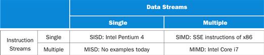
FIGURE 6.2 Hardware categorization and examples based on number of instruction streams and data streams: SISD, SIMD, MISD, and MIMD.
While it is possible to write separate programs that run on different processors on a MIMD computer and yet work together for a grander, coordinated goal, programmers normally write a single program that runs on all processors of an MIMD computer, relying on conditional statements when different processors should execute different sections of code. This style is called Single Program Multiple Data (SPMD), but it is just the normal way to program a MIMD computer.
SPMD
Single Program, Multiple Data streams. The conventional MIMD programming model, where a single program runs across all processors.
The closest we can come to multiple instruction streams and single data stream (MISD) processor might be a “stream processor” that would perform a series of computations on a single data stream in a pipelined fashion: parse the input from the network, decrypt the data, decompress it, search for match, and so on. The inverse of MISD is much more popular. SIMD computers operate on vectors of data. For example, a single SIMD instruction might add 64 numbers by sending 64 data streams to 64 ALUs to form 64 sums within a single clock cycle. The subword parallel instructions that we saw in Sections 3.6 and 3.7 are another example of SIMD; indeed, the middle letter of Intel’s SSE acronym stands for SIMD.
SIMD
or Single Instruction stream, Multiple Data streams. The same instruction is applied to many data streams, as in a vector processor.
The virtues of SIMD are that all the parallel execution units are synchronized and they all respond to a single instruction that emanates from a single program counter (PC). From a programmer’s perspective, this is close to the already familiar SISD. Although every unit will be executing the same instruction, each execution unit has its own address registers, and so each unit can have different data addresses. Thus, in terms of Figure 6.1, a sequential application might be compiled to run on serial hardware organized as a SISD or in parallel hardware that was organized as a SIMD.
The original motivation behind SIMD was to amortize the cost of the control unit over dozens of execution units. Another advantage is the reduced instruction bandwidth and space—SIMD needs only one copy of the code that is being simultaneously executed, while message-passing MIMDs may need a copy in every processor, and shared memory MIMD will need multiple instruction caches.
SIMD works best when dealing with arrays in for loops. Hence, for parallelism to work in SIMD, there must be a great deal of identically structured data, which is called data-level parallelism. SIMD is at its weakest in case or switch statements, where each execution unit must perform a different operation on its data, depending on what data it has. Execution units with the wrong data must be disabled so that units with proper data may continue. If there are n cases, in these situations SIMD processors essentially run at 1/nth of peak performance.
data-level parallelism
Parallelism achieved by performing the same operation on independent data.
The so-called array processors that inspired the SIMD category have faded into history (see ![]() Section 6.15 online), but two current interpretations of SIMD remain active today.
Section 6.15 online), but two current interpretations of SIMD remain active today.
SIMD in x86: Multimedia Extensions
As described in Chapter 3, subword parallelism for narrow integer data was the original inspiration of the Multimedia Extension (MMX) instructions of the x86 in 1996. As Moore’s Law continued, more instructions were added, leading first to Streaming SIMD Extensions (SSE) and now Advanced Vector Extensions (AVX). AVX supports the simultaneous execution of four 64-bit floating-point numbers. The width of the operation and the registers is encoded in the opcode of these multimedia instructions. As the data width of the registers and operations grew, the number of opcodes for multimedia instructions exploded, and now there are hundreds of SSE and AVX instructions (see Chapter 3).
Vector
An older and, as we shall see, more elegant interpretation of SIMD is called a vector architecture, which has been closely identified with computers designed by Seymour Cray starting in the 1970s. It is also a great match to problems with lots of data-level parallelism. Rather than having 64 ALUs perform 64 additions simultaneously, like the old array processors, the vector architectures pipelined the ALU to get good performance at lower cost. The basic philosophy of vector architecture is to collect data elements from memory, put them in order into a large set of registers, operate on them sequentially in registers using pipelined execution units, and then write the results back to memory. A key feature of vector architectures is then a set of vector registers. Thus, a vector architecture might have 32 vector registers, each with 64 64-bit elements.

Comparing Vector to Conventional Code
Example
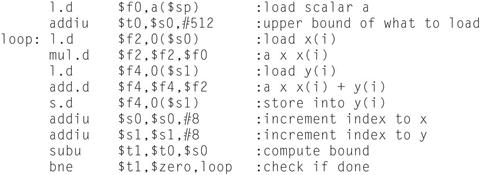
Suppose we extend the MIPS instruction set architecture with vector instructions and vector registers. Vector operations use the same names as MIPS operations, but with the letter “V” appended. For example, addv.d adds two double-precision vectors. The vector instructions take as their input either a pair of vector registers (addv.d) or a vector register and a scalar register (addvs.d). In the latter case, the value in the scalar register is used as the input for all operations—the operation addvs.d will add the contents of a scalar register to each element in a vector register. The names lvand sv denote vector load and vector store, and they load or store an entire vector of double-precision data. One operand is the vector register to be loaded or stored; the other operand, which is a MIPS general-purpose register, is the starting address of the vector in memory. Given this short description, show the conventional MIPS code versus the vector MIPS code for
![]()
where X and Y are vectors of 64 double precision floating-point numbers, initially resident in memory, and a is a scalar double precision variable. (This example is the so-called DAXPY loop that forms the inner loop of the Linpack benchmark; DAXPY stands for double precision a×Xplus Y.). Assume that the starting addresses of X and Y are in $s0 and $s1, respectively.
Answer
Here is the conventional MIPS code for DAXPY:
Here is the vector MIPS code for DAXPY:
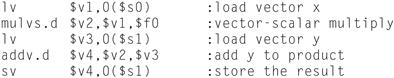
There are some interesting comparisons between the two code segments in this example. The most dramatic is that the vector processor greatly reduces the dynamic instruction bandwidth, executing only 6 instructions versus almost 600 for the traditional MIPS architecture. This reduction occurs both because the vector operations work on 64 elements at a time and because the overhead instructions that constitute nearly half the loop on MIPS are not present in the vector code. As you might expect, this reduction in instructions fetched and executed saves energy.
Another important difference is the frequency of pipeline hazards (Chapter 4). In the straightforward MIPS code, every add.d must wait for a mul.d, every s.d must wait for the add.d and every add.dandmul.dmust wait on l.d. On the vector processor, each vector instruction will only stall for the first element in each vector, and then subsequent elements will flow smoothly down the pipeline. Thus, pipeline stalls are required only once per vector operation, rather than once per vector element. In this example, the pipeline stall frequency on MIPS will be about 64 times higher than it is on the vector version of MIPS. The pipeline stalls can be reduced on MIPS by using loop unrolling (see Chapter 4). However, the large difference in instruction bandwidth cannot be reduced.
Since the vector elements are independent, they can be operated on in parallel, much like subword parallelism for AVX instructions. All modern vector computers have vector functional units with multiple parallel pipelines (called vector lanes; see Figures 6.2 and 6.3) that can produce two or more results per clock cycle.
Elaboration
The loop in the example above exactly matched the vector length. When loops are shorter, vector architectures use a register that reduces the length of vector operations. When loops are larger, we add bookkeeping code to iterate full-length vector operations and to handle the leftovers. This latter process is called strip mining.
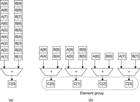
FIGURE 6.3 Using multiple functional units to improve the performance of a single vector add instruction, C=A+B.
The vector processor (a) on the left has a single add pipeline and can complete one addition per cycle. The vector processor (b) on the right has four add pipelines or lanes and can complete four additions per cycle. The elements within a single vector add instruction are interleaved across the four lanes.
Vector versus Scalar
Vector instructions have several important properties compared to conventional instruction set architectures, which are called scalar architectures in this context:
■ A single vector instruction specifies a great deal of work—it is equivalent to executing an entire loop. The instruction fetch and decode bandwidth needed is dramatically reduced.
■ By using a vector instruction, the compiler or programmer indicates that the computation of each result in the vector is independent of the computation of other results in the same vector, so hardware does not have to check for data hazards within a vector instruction.
■ Vector architectures and compilers have a reputation of making it much easier than when using MIMD multiprocessors to write efficient applications when they contain data-level parallelism.
■ Hardware need only check for data hazards between two vector instructions once per vector operand, not once for every element within the vectors. Reduced checking can save energy as well as time.
■ Vector instructions that access memory have a known access pattern. If the vector’s elements are all adjacent, then fetching the vector from a set of heavily interleaved memory banks works very well. Thus, the cost of the latency to main memory is seen only once for the entire vector, rather than once for each word of the vector.
■ Because an entire loop is replaced by a vector instruction whose behavior is predetermined, control hazards that would normally arise from the loop branch are nonexistent.
■ The savings in instruction bandwidth and hazard checking plus the efficient use of memory bandwidth give vector architectures advantages in power and energy versus scalar architectures.
For these reasons, vector operations can be made faster than a sequence of scalar operations on the same number of data items, and designers are motivated to include vector units if the application domain can often use them.
Vector versus Multimedia Extensions
Like multimedia extensions found in the x86 AVX instructions, a vector instruction specifies multiple operations. However, multimedia extensions typically specify a few operations while vector specifies dozens of operations. Unlike multimedia extensions, the number of elements in a vector operation is not in the opcode but in a separate register. This distinction means different versions of the vector architecture can be implemented with a different number of elements just by changing the contents of that register and hence retain binary compatibility. In contrast, a new large set of opcodes is added each time the “vector” length changes in the multimedia extension architecture of the x86: MMX, SSE, SSE2, AVX, AVX2, ….
Also unlike multimedia extensions, the data transfers need not be contiguous. Vectors support both strided accesses, where the hardware loads every nth data element in memory, and indexed accesses, where hardware finds the addresses of the items to be loaded in a vector register. Indexed accesses are also called gather-scatter, in that indexed loads gather elements from main memory into contiguous vector elements and indexed stores scatter vector elements across main memory.
Like multimedia extensions, vector architectures easily capture the flexibility in data widths, so it is easy to make a vector operation work on 32 64-bit data elements or 64 32-bit data elements or 128 16-bit data elements or 256 8-bit data elements. The parallel semantics of a vector instruction allows an implementation to execute these operations using a deeply pipelined functional unit, an array of parallel functional units, or a combination of parallel and pipelined functional units. Figure 6.3 illustrates how to improve vector performance by using parallel pipelines to execute a vector add instruction.
Vector arithmetic instructions usually only allow element N of one vector register to take part in operations with element N from other vector registers. This dramatically simplifies the construction of a highly parallel vector unit, which can be structured as multiple parallel vector lanes. As with a traffic highway, we can increase the peak throughput of a vector unit by adding more lanes. Figure 6.4 shows the structure of a four-lane vector unit. Thus, going to four lanes from one lane reduces the number of clocks per vector instruction by roughly a factor of four. For multiple lanes to be advantageous, both the applications and the architecture must support long vectors. Otherwise, they will execute so quickly that you’ll run out of instructions, requiring instruction level parallel techniques like those in Chapter 4 to supply enough vector instructions.
vector lane
One or more vector functional units and a portion of the vector register file. Inspired by lanes on highways that increase traffic speed, multiple lanes execute vector operations simultaneously.
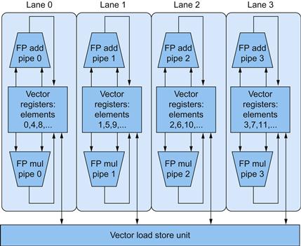
FIGURE 6.4 Structure of a vector unit containing four lanes.
The vector-register storage is divided across the lanes, with each lane holding every fourth element of each vector register. The figure shows three vector functional units: an FP add, an FP multiply, and a load-store unit. Each of the vector arithmetic units contains four execution pipelines, one per lane, which acts in concert to complete a single vector instruction. Note how each section of the vector-register file only needs to provide enough read and write ports (see Chapter 4) for functional units local to its lane.
Generally, vector architectures are a very efficient way to execute data parallel processing programs; they are better matches to compiler technology than multimedia extensions; and they are easier to evolve over time than the multimedia extensions to the x86 architecture.
Given these classic categories, we next see how to exploit parallel streams of instructions to improve the performance of a single processor, which we will reuse with multiple processors.
Check Yourself
True or false: As exemplified in the x86, multimedia extensions can be thought of as a vector architecture with short vectors that supports only contiguous vector data transfers.
Elaboration
Given the advantages of vector, why aren’t they more popular outside high-performance computing? There were concerns about the larger state for vector registers increasing context switch time and the difficulty of handling page faults in vector loads and stores, and SIMD instructions achieved some of the benefits of vector instructions. In addition, as long as advances in instruction level parallelism could deliver on the performance promise of Moore’s Law, there was little reason to take the chance of changing architecture styles.
Elaboration
Another advantage of vector and multimedia extensions is that it is relatively easy to extend a scalar instruction set architecture with these instructions to improve performance of data parallel operations.
Elaboration
The Haswell-generation x86 processors from Intel support AVX2, which has a gather operation but not a scatter operation.
6.4 Hardware Multithreading
A related concept to MIMD, especially from the programmer’s perspective, is hardware multithreading. While MIMD relies on multiple processes or threads to try to keep multiple processors busy, hardware multithreading allows multiple threads to share the functional units of a single processor in an overlapping fashion to try to utilize the hardware resources efficiently. To permit this sharing, the processor must duplicate the independent state of each thread. For example, each thread would have a separate copy of the register file and the program counter. The memory itself can be shared through the virtual memory mechanisms, which already support multi-programming. In addition, the hardware must support the ability to change to a different thread relatively quickly. In particular, a thread switch should be much more efficient than a process switch, which typically requires hundreds to thousands of processor cycles while a thread switch can be instantaneous.
hardware multithreading
Increasing utilization of a processor by switching to another thread when one thread is stalled.
thread
A thread includes the program counter, the register state, and the stack. It is a lightweight process; whereas threads commonly share a single address space, processes don’t.
process
A process includes one or more threads, the address space, and the operating system state. Hence, a process switch usually invokes the operating system, but not a thread switch.
There are two main approaches to hardware multithreading. Fine-grained multithreading switches between threads on each instruction, resulting in interleaved execution of multiple threads. This interleaving is often done in a round-robin fashion, skipping any threads that are stalled at that clock cycle. To make fine-grained multithreading practical, the processor must be able to switch threads on every clock cycle. One advantage of fine-grained multithreading is that it can hide the throughput losses that arise from both short and long stalls, since instructions from other threads can be executed when one thread stalls. The primary disadvantage of fine-grained multithreading is that it slows down the execution of the individual threads, since a thread that is ready to execute without stalls will be delayed by instructions from other threads.
fine-grained multithreading
A version of hardware multithreading that implies switching between threads after every instruction.
Coarse-grained multithreading was invented as an alternative to fine-grained multithreading. Coarse-grained multithreading switches threads only on costly stalls, such as last-level cache misses. This change relieves the need to have thread switching be extremely fast and is much less likely to slow down the execution of an individual thread, since instructions from other threads will only be issued when a thread encounters a costly stall. Coarse-grained multithreading suffers, however, from a major drawback: it is limited in its ability to overcome throughput losses, especially from shorter stalls. This limitation arises from the pipeline start-up costs of coarse-grained multithreading. Because a processor with coarse-grained multithreading issues instructions from a single thread, when a stall occurs, the pipeline must be emptied or frozen. The new thread that begins executing after the stall must fill the pipeline before instructions will be able to complete. Due to this start-up overhead, coarse-grained multithreading is much more useful for reducing the penalty of high-cost stalls, where pipeline refill is negligible compared to the stall time.
coarse-grained multithreading
A version of hardware multithreading that implies switching between threads only after significant events, such as a last-level cache miss.
Simultaneous multithreading (SMT) is a variation on hardware multithreading that uses the resources of a multiple-issue, dynamically scheduled pipelined processor to exploit thread-level parallelism at the same time it exploits instruction-level parallelism (see Chapter 4). The key insight that motivates SMT is that multiple-issue processors often have more functional unit parallelism available than most single threads can effectively use. Furthermore, with register renaming and dynamic scheduling (see Chapter 4), multiple instructions from independent threads can be issued without regard to the dependences among them; the resolution of the dependences can be handled by the dynamic scheduling capability.
simultaneous multithreading (SMT)
A version of multithreading that lowers the cost of multithreading by utilizing the resources needed for multiple issue, dynamically scheduled microarchitecture.
Since SMT relies on the existing dynamic mechanisms, it does not switch resources every cycle. Instead, SMT is always executing instructions from multiple threads, leaving it up to the hardware to associate instruction slots and renamed registers with their proper threads.
Figure 6.5 conceptually illustrates the differences in a processor’s ability to exploit superscalar resources for the following processor configurations. The top portion shows how four threads would execute independently on a superscalar with no multithreading support. The bottom portion shows how the four threads could be combined to execute on the processor more efficiently using three multithreading options:
■ A superscalar with coarse-grained multithreading
■ A superscalar with fine-grained multithreading
■ A superscalar with simultaneous multithreading
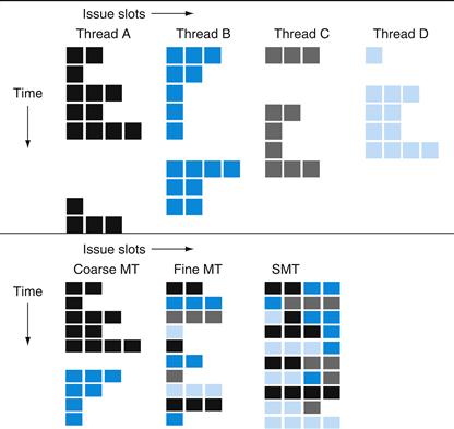
FIGURE 6.5 How four threads use the issue slots of a superscalar processor in different approaches.
The four threads at the top show how each would execute running alone on a standard superscalar processor without multithreading support. The three examples at the bottom show how they would execute running together in three multithreading options. The horizontal dimension represents the instruction issue capability in each clock cycle. The vertical dimension represents a sequence of clock cycles. An empty (white) box indicates that the corresponding issue slot is unused in that clock cycle. The shades of gray and color correspond to four different threads in the multithreading processors. The additional pipeline start-up effects for coarse multithreading, which are not illustrated in this figure, would lead to further loss in throughput for coarse multithreading.
In the superscalar without hardware multithreading support, the use of issue slots is limited by a lack of instruction-level parallelism. In addition, a major stall, such as an instruction cache miss, can leave the entire processor idle.
In the coarse-grained multithreaded superscalar, the long stalls are partially hidden by switching to another thread that uses the resources of the processor. Although this reduces the number of completely idle clock cycles, the pipeline start-up overhead still leads to idle cycles, and limitations to ILP means all issue slots will not be used. In the fine-grained case, the interleaving of threads mostly eliminates idle clock cycles. Because only a single thread issues instructions in a given clock cycle, however, limitations in instruction-level parallelism still lead to idle slots within some clock cycles.
In the SMT case, thread-level parallelism and instruction-level parallelism are both exploited, with multiple threads using the issue slots in a single clock cycle. Ideally, the issue slot usage is limited by imbalances in the resource needs and resource availability over multiple threads. In practice, other factors can restrict how many slots are used. Although Figure 6.5 greatly simplifies the real operation of these processors, it does illustrate the potential performance advantages of multithreading in general and SMT in particular.
Figure 6.6 plots the performance and energy benefits of multithreading on a single processors of the Intel Core i7 960, which has hardware support for two threads. The average speedup is 1.31, which is not bad given the modest extra resources for hardware multithreading. The average improvement in energy efficiency is 1.07, which is excellent. In general, you’d be happy with a performance speedup being energy neutral.
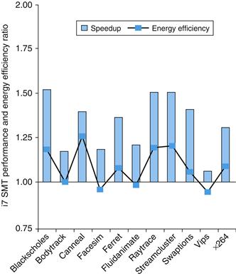
FIGURE 6.6 The speedup from using multithreading on one core on an i7 processor averages 1.31 for the PARSEC benchmarks (see ![]() Section 6.9) and the energy efficiency improvement is 1.07. This data was collected and analyzed by Esmaeilzadeh et. al. [2011].
Section 6.9) and the energy efficiency improvement is 1.07. This data was collected and analyzed by Esmaeilzadeh et. al. [2011].
Now that we have seen how multiple threads can utilize the resources of a single processor more effectively, we next show how to use them to exploit multiple processors.
Check Yourself
1. True or false: Both multithreading and multicore rely on parallelism to get more efficiency from a chip.
2. True or false: Simultaneous multithreading (SMT) uses threads to improve resource utilization of a dynamically scheduled, out-of-order processor.
6.5 Multicore and Other Shared Memory Multiprocessors
While hardware multithreading improved the efficiency of processors at modest cost, the big challenge of the last decade has been to deliver on the performance potential of Moore’s Law by efficiently programming the increasing number of processors per chip.
Given the difficulty of rewriting old programs to run well on parallel hardware, a natural question is: what can computer designers do to simplify the task? One answer was to provide a single physical address space that all processors can share, so that programs need not concern themselves with where their data is, merely that programs may be executed in parallel. In this approach, all variables of a program can be made available at any time to any processor. The alternative is to have a separate address space per processor that requires that sharing must be explicit; we’ll describe this option in the Section 6.7. When the physical address space is common then the hardware typically provides cache coherence to give a consistent view of the shared memory (see Section 5.8).
As mentioned above, a shared memory multiprocessor (SMP) is one that offers the programmer a single physical address space across all processors—which is nearly always the case for multicore chips—although a more accurate term would have been shared-address multiprocessor. Processors communicate through shared variables in memory, with all processors capable of accessing any memory location via loads and stores. Figure 6.7 shows the classic organization of an SMP. Note that such systems can still run independent jobs in their own virtual address spaces, even if they all share a physical address space.
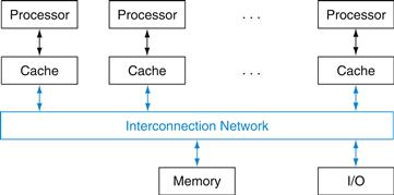
FIGURE 6.7 Classic organization of a shared memory multiprocessor.
Single address space multiprocessors come in two styles. In the first style, the latency to a word in memory does not depend on which processor asks for it. Such machines are called uniform memory access (UMA) multiprocessors. In the second style, some memory accesses are much faster than others, depending on which processor asks for which word, typically because main memory is divided and attached to different microprocessors or to different memory controllers on the same chip. Such machines are called nonuniform memory access (NUMA) multiprocessors. As you might expect, the programming challenges are harder for a NUMA multiprocessor than for a UMA multiprocessor, but NUMA machines can scale to larger sizes and NUMAs can have lower latency to nearby memory.
uniform memory access (UMA)
A multiprocessor in which latency to any word in main memory is about the same no matter which processor requests the access.
nonuniform memory access (NUMA)
A type of single address space multiprocessor in which some memory accesses are much faster than others depending on which processor asks for which word.
As processors operating in parallel will normally share data, they also need to coordinate when operating on shared data; otherwise, one processor could start working on data before another is finished with it. This coordination is called synchronization, which we saw in Chapter 2. When sharing is supported with a single address space, there must be a separate mechanism for synchronization. One approach uses a lock for a shared variable. Only one processor at a time can acquire the lock, and other processors interested in shared data must wait until the original processor unlocks the variable. Section 2.11 of Chapter 2describes the instructions for locking in the MIPS instruction set.
synchronization
The process of coordinating the behavior of two or more processes, which may be running on different processors.
lock
A synchronization device that allows access to data to only one processor at a time.
A Simple Parallel Processing Program for a Shared Address Space
Example
Suppose we want to sum 64,000 numbers on a shared memory multiprocessor computer with uniform memory access time. Let’s assume we have 64 processors.
Answer
The first step is to ensure a balanced load per processor, so we split the set of numbers into subsets of the same size. We do not allocate the subsets to a different memory space, since there is a single memory space for this machine; we just give different starting addresses to each processor. Pn is the number that identifies the processor, between 0 and 63. All processors start the program by running a loop that sums their subset of numbers:
sum[Pn] = 0;
for (i = 1000*Pn; i < 1000*(Pn+1); i += 1)
sum[Pn] += A[i]; /*sum the assigned areas*/
(Note the C code i += 1 is just a shorter way to say i = i + 1.)
The next step is to add these 64 partial sums. This step is called a reduction, where we divide to conquer. Half of the processors add pairs of partial sums, and then a quarter add pairs of the new partial sums, and so on until we have the single, final sum. Figure 6.8 illustrates the hierarchical nature of this reduction.
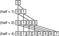
FIGURE 6.8 The last four levels of a reduction that sums results from each processor, from bottom to top.
For all processors whose number i is less than half, add the sum produced by processor number (i+half) to its sum.
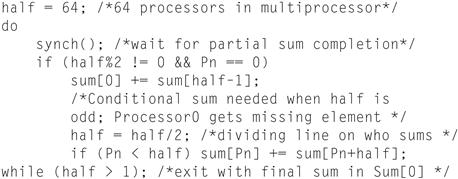
In this example, the two processors must synchronize before the “consumer” processor tries to read the result from the memory location written by the “producer” processor; otherwise, the consumer may read the old value of the data. We want each processor to have its own version of the loop counter variable i, so we must indicate that it is a “private” variable. Here is the code (halfis private also):
reduction
A function that processes a data structure and returns a single value.
Hardware/Software Interface
Given the long-term interest in parallel programming, there have been hundreds of attempts to build parallel programming systems. A limited but popular example is OpenMP. It is just an Application Programmer Interface (API) along with a set of compiler directives, environment variables, and runtime library routines that can extend standard programming languages. It offers a portable, scalable, and simple programming model for shared memory multiprocessors. Its primary goal is to parallelize loops and to perform reductions.
OpenMP
An API for shared memory multiprocessing in C, C++, or Fortran that runs on UNIX and Microsoft platforms. It includes compiler directives, a library, and runtime directives.
Most C compilers already have support for OpenMP. The command to uses the OpenMP API with the UNIX C compiler is just:
cc –fopenmp foo.c
OpenMP extends C using pragmas, which are just commands to the C macro preprocessor like #define and #include. To set the number of processors we want to use to be 64, as we wanted in the example above, we just use the command
#define P 64 /* define a constant that we’ll use a few times */
#pragma omp parallel num_threads(P)
That is, the runtime libraries should use 64 parallel threads.
To turn the sequential for loop into a parallel for loop that divides the work equally between all the threads that we told it to use, we just write (assuming sum is initialized to 0)
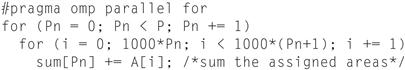
To perform the reduction, we can use another command that tells OpenMP what the reduction operator is and what variable you need to use to place the result of the reduction.
#pragma omp parallel for reduction(+ : FinalSum)
for (i = 0; i < P; i += 1)
FinalSum += sum[i]; /* Reduce to a single number */
Note that it is now up to the OpenMP library to find efficient code to sum 64 numbers efficiently using 64 processors.
While OpenMP makes it easy to write simple parallel code, it is not very helpful with debugging, so many parallel programmers use more sophisticated parallel programming systems than OpenMP, just as many programmers today use more productive languages than C.
Given this tour of classic MIMD hardware and software, our next path is a more exotic tour of a type of MIMD architecture with a different heritage and thus a very different perspective on the parallel programming challenge.
Check Yourself
True or false: Shared memory multiprocessors cannot take advantage of task-level parallelism.
Elaboration
Some writers repurposed the acronym SMP to mean symmetric multiprocessor, to indicate that the latency from processor to memory was about the same for all processors. This shift was done to contrast them from large-scale NUMA multiprocessors, as both classes used a single address space. As clusters proved much more popular than large-scale NUMA multiprocessors, in this book we restore SMP to its original meaning, and use it to contrast against that use multiple address spaces, such as clusters.
Elaboration
An alternative to sharing the physical address space would be to have separate physical address spaces but share a common virtual address space, leaving it up to the operating system to handle communication. This approach has been tried, but it has too high an overhead to offer a practical shared memory abstraction to the performance-oriented programmer.
6.6 Introduction to Graphics Processing Units
The original justification for adding SIMD instructions to existing architectures was that many microprocessors were connected to graphics displays in PCs and workstations, so an increasing fraction of processing time was used for graphics. As Moore’s Law increased the number of transistors available to microprocessors, it therefore made sense to improve graphics processing.
A major driving force for improving graphics processing was the computer game industry, both on PCs and in dedicated game consoles such as the Sony PlayStation. The rapidly growing game market encouraged many companies to make increasing investments in developing faster graphics hardware, and this positive feedback loop led graphics processing to improve at a faster rate than general-purpose processing in mainstream microprocessors.
Given that the graphics and game community had different goals than the microprocessor development community, it evolved its own style of processing and terminology. As the graphics processors increased in power, they earned the name Graphics Processing Units or GPUs to distinguish themselves from CPUs.
For a few hundred dollars, anyone can buy a GPU today with hundreds of parallel floating-point units, which makes high-performance computing more accessible. The interest in GPU computing blossomed when this potential was combined with a programming language that made GPUs easier to program. Hence, many programmers of scientific and multimedia applications today are pondering whether to use GPUs or CPUs.
(This section concentrates on using GPUs for computing. To see how GPU computing combines with the traditional role of graphics acceleration, see ![]() Appendix C.)
Appendix C.)
Here are some of the key characteristics as to how GPUs vary from CPUs:
■ GPUs are accelerators that supplement a CPU, so they do not need be able to perform all the tasks of a CPU. This role allows them to dedicate all their resources to graphics. It’s fine for GPUs to perform some tasks poorly or not at all, given that in a system with both a CPU and a GPU, the CPU can do them if needed.
■ The GPU problems sizes are typically hundreds of megabytes to gigabytes, but not hundreds of gigabytes to terabytes.
These differences led to different styles of architecture:
■ Perhaps the biggest difference is that GPUs do not rely on multilevel caches to overcome the long latency to memory, as do CPUs. Instead, GPUs rely on hardware multithreading (Section 6.4) to hide the latency to memory. That is, between the time of a memory request and the time that data arrives, the GPU executes hundreds or thousands of threads that are independent of that request.
■ The GPU memory is thus oriented toward bandwidth rather than latency. There are even special graphics DRAM chips for GPUs that are wider and have higher bandwidth than DRAM chips for CPUs. In addition, GPU memories have traditionally had smaller main memories than conventional microprocessors. In 2013, GPUs typically have 4 to 6 GiB or less, while CPUs have 32 to 256 GiB. Finally, keep in mind that for general-purpose computation, you must include the time to transfer the data between CPU memory and GPU memory, since the GPU is a coprocessor.
■ Given the reliance on many threads to deliver good memory bandwidth, GPUs can accommodate many parallel processors (MIMD) as well as many threads. Hence, each GPU processor is more highly multithreaded than a typical CPU, plus they have more processors.
Hardware/Software Interface
Although GPUs were designed for a narrower set of applications, some programmers wondered if they could specify their applications in a form that would let them tap the high potential performance of GPUs. After tiring of trying to specify their problems using the graphics APIs and languages, they developed C-inspired programming languages to allow them to write programs directly for the GPUs. An example is NVIDIA’s CUDA (Compute Unified Device Architecture), which enables the programmer to write C programs to execute on GPUs, albeit with some restrictions. ![]() Appendix C gives examples of CUDA code. (OpenCL is a multi-company initiative to develop a portable programming language that provides many of the benefits of CUDA.)
Appendix C gives examples of CUDA code. (OpenCL is a multi-company initiative to develop a portable programming language that provides many of the benefits of CUDA.)
NVIDIA decided that the unifying theme of all these forms of parallelism is the CUDA Thread. Using this lowest level of parallelism as the programming primitive, the compiler and the hardware can gang thousands of CUDA Threads together to utilize the various styles of parallelism within a GPU: multithreading, MIMD, SIMD, and instruction-level parallelism. These threads are blocked together and executed in groups of 32 at a time. A multithreaded processor inside a GPU executes these blocks of threads, and a GPU consists of 8 to 32 of these multithreaded processors.
An Introduction to the NVIDIA GPU Architecture
We use NVIDIA systems as our example as they are representative of GPU architectures. Specifically, we follow the terminology of the CUDA parallel programming language and use the Fermi architecture as the example.
Like vector architectures, GPUs work well only with data-level parallel problems. Both styles have gather-scatter data transfers, and GPU processors have even more registers than do vector processors. Unlike most vector architectures, GPUs also rely on hardware multithreading within a single multithreaded SIMD processor to hide memory latency (see Section 6.4).
A multithreaded SIMD processor is similar to a Vector Processor, but the former has many parallel functional units instead of just a few that are deeply pipelined, as does the latter.
As mentioned above, a GPU contains a collection of multithreaded SIMD processors; that is, a GPU is a MIMD composed of multithreaded SIMD processors. For example, NVIDIA has four implementations of the Fermi architecture at different price points with 7, 11, 14, or 15 multithreaded SIMD processors. To provide transparent scalability across models of GPUs with differing number of multithreaded SIMD processors, the Thread Block Scheduler hardware assigns blocks of threads to multithreaded SIMD processors. Figure 6.9 shows a simplified block diagram of a multithreaded SIMD processor.
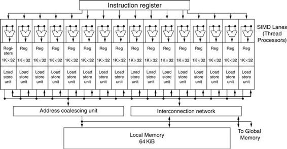
FIGURE 6.9 Simplified block diagram of the datapath of a multithreaded SIMD Processor.
It has 16 SIMD lanes. The SIMD Thread Scheduler has many independent SIMD threads that it chooses from to run on this processor.
Dropping down one more level of detail, the machine object that the hardware creates, manages, schedules, and executes is a thread of SIMD instructions, which we will also call a SIMD thread. It is a traditional thread, but it contains exclusively SIMD instructions. These SIMD threads have their own program counters and they run on a multithreaded SIMD processor. The SIMD Thread Scheduler includes a controller that lets it know which threads of SIMD instructions are ready to run, and then it sends them off to a dispatch unit to be run on the multithreaded SIMD processor. It is identical to a hardware thread scheduler in a traditional multithreaded processor (see Section 6.4), except that it is scheduling threads of SIMD instructions. Thus, GPU hardware has two levels of hardware schedulers:
1. The Thread Block Scheduler that assigns blocks of threads to multithreaded SIMD processors, and
2. the SIMD Thread Scheduler within a SIMD processor, which schedules when SIMD threads should run.
The SIMD instructions of these threads are 32 wide, so each thread of SIMD instructions would compute 32 of the elements of the computation. Since the thread consists of SIMD instructions, the SIMD processor must have parallel functional units to perform the operation. We call them SIMD Lanes, and they are quite similar to the Vector Lanes in Section 6.3.
Elaboration
The number of lanes per SIMD processor varies across GPU generations. With Fermi, each 32-wide thread of SIMD instructions is mapped to 16 SIMD Lanes, so each SIMD instruction in a thread of SIMD instructions takes two clock cycles to complete. Each thread of SIMD instructions is executed in lock step. Staying with the analogy of a SIMD processor as a vector processor, you could say that it has 16 lanes, and the vector length would be 32. This wide but shallow nature is why we use the term SIMD processor instead of vector processor, as it is more intuitive.
Since by definition the threads of SIMD instructions are independent, the SIMD Thread Scheduler can pick whatever thread of SIMD instructions is ready, and need not stick with the next SIMD instruction in the sequence within a single thread. Thus, using the terminology of Section 6.4, it uses fine-grained multithreading.
To hold these memory elements, a Fermi SIMD processor has an impressive 32,768 32-bit registers. Just like a vector processor, these registers are divided logically across the vector lanes or, in this case, SIMD Lanes. Each SIMD Thread is limited to no more than 64 registers, so you might think of a SIMD Thread as having up to 64 vector registers, with each vector register having 32 elements and each element being 32 bits wide.
Since Fermi has 16 SIMD Lanes, each contains 2048 registers. Each CUDA Thread gets one element of each of the vector registers. Note that a CUDA thread is just a vertical cut of a thread of SIMD instructions, corresponding to one element executed by one SIMD Lane. Beware that CUDA Threads are very different from POSIX threads; you can’t make arbitrary system calls or synchronize arbitrarily in a CUDA Thread.
NVIDIA GPU Memory Structures
Figure 6.10 shows the memory structures of an NVIDIA GPU. We call the on-chip memory that is local to each multithreaded SIMD processor Local Memory. It is shared by the SIMD Lanes within a multithreaded SIMD processor, but this memory is not shared between multithreaded SIMD processors. We call the off-chip DRAM shared by the whole GPU and all thread blocks GPU Memory.
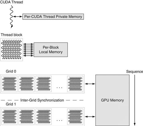
FIGURE 6.10 GPU Memory structures.
GPU Memory is shared by the vectorized loops. All threads of SIMD instructions within a thread block share Local Memory.
Rather than rely on large caches to contain the whole working sets of an application, GPUs traditionally use smaller streaming caches and rely on extensive multithreading of threads of SIMD instructions to hide the long latency to DRAM, since their working sets can be hundreds of megabytes. Thus, they will not fit in the last level cache of a multicore microprocessor. Given the use of hardware multithreading to hide DRAM latency, the chip area used for caches in system processors is spent instead on computing resources and on the large number of registers to hold the state of the many threads of SIMD instructions.
Elaboration
While hiding memory latency is the underlying philosophy, note that the latest GPUs and vector processors have added caches. For example, the recent Fermi architecture has added caches, but they are thought of as either bandwidth filters to reduce demands on GPU Memory or as accelerators for the few variables whose latency cannot be hidden by multithreading. Local memory for stack frames, function calls, and register spilling is a good match to caches, since latency matters when calling a function. Caches can also save energy, since on-chip cache accesses take much less energy than accesses to multiple, external DRAM chips.
Putting GPUs into Perspective
At a high level, multicore computers with SIMD instruction extensions do share similarities with GPUs. Figure 6.11 summarizes the similarities and differences. Both are MIMDs whose processors use multiple SIMD lanes, although GPUs have more processors and many more lanes. Both use hardware multithreading to improve processor utilization, although GPUs have hardware support for many more threads. Both use caches, although GPUs use smaller streaming caches and multicore computers use large multilevel caches that try to contain whole working sets completely. Both use a 64-bit address space, although the physical main memory is much smaller in GPUs. While GPUs support memory protection at the page level, they do not yet support demand paging.
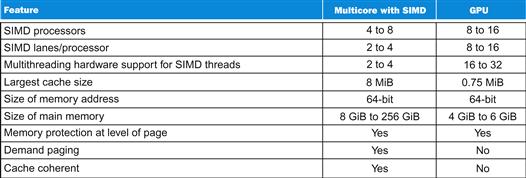
FIGURE 6.11 Similarities and differences between multicore with Multimedia SIMD extensions and recent GPUs.
SIMD processors are also similar to vector processors. The multiple SIMD processors in GPUs act as independent MIMD cores, just as many vector computers have multiple vector processors. This view would consider the Fermi GTX 580 as a 16-core machine with hardware support for multithreading, where each core has 16 lanes. The biggest difference is multithreading, which is fundamental to GPUs and missing from most vector processors.
GPUs and CPUs do not go back in computer architecture genealogy to a common ancestor; there is no Missing Link that explains both. As a result of this uncommon heritage, GPUs have not used the terms common in the computer architecture community, which has led to confusion about what GPUs are and how they work. To help resolve the confusion, Figure 6.12 (from left to right) lists the more descriptive term used in this section, the closest term from mainstream computing, the official NVIDIA GPU term in case you are interested, and then a short description of the term. This “GPU Rosetta Stone” may help relate this section and ideas to more conventional GPU descriptions, such as those found in ![]() Appendix C.
Appendix C.
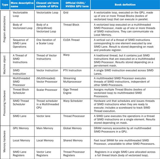
FIGURE 6.12 Quick guide to GPU terms.
We use the first column for hardware terms. Four groups cluster these 12 terms. From top to bottom: Program Abstractions, Machine Objects, Processing Hardware, and Memory Hardware.
While GPUs are moving toward mainstream computing, they can’t abandon their responsibility to continue to excel at graphics. Thus, the design of GPUs may make more sense when architects ask, given the hardware invested to do graphics well, how can we supplement it to improve the performance of a wider range of applications?
Having covered two different styles of MIMD that have a shared address space, we next introduce parallel processors where each processor has its own private address space, which makes it much easier to build much larger systems. The Internet services that you use every day depend on these large scale systems.
Elaboration
While the GPU was introduced as having a separate memory from the CPU, both AMD and Intel have announced “fused” products that combine GPUs and CPUs to share a single memory. The challenge will be to maintain the high bandwidth memory in a fused architecture that has been a foundation of GPUs.
Check Yourself
True or false: GPUs rely on graphics DRAM chips to reduce memory latency and thereby increase performance on graphics applications.
6.7 Clusters, Warehouse Scale Computers, and Other Message-Passing Multiprocessors
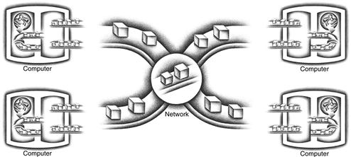
The alternative approach to sharing an address space is for the processors to each have their own private physical address space. Figure 6.13 shows the classic organization of a multiprocessor with multiple private address spaces. This alternative multiprocessor must communicate via explicit message passing, which traditionally is the name of such style of computers. Provided the system has routines to sendand receive messages, coordination is built in with message passing, since one processor knows when a message is sent, and the receiving processor knows when a message arrives. If the sender needs confirmation that the message has arrived, the receiving processor can then send an acknowledgment message back to the sender.
message passing
Communicating between multiple processors by explicitly sending and receiving information.
send message routine
A routine used by a processor in machines with private memories to pass a message to another processor.
receive message routine
A routine used by a processor in machines with private memories to accept a message from another processor.
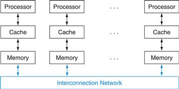
FIGURE 6.13 Classic organization of a multiprocessor with multiple private address spaces, traditionally called a message-passing multiprocessor.
Note that unlike the SMP in Figure 6.7, the interconnection network is not between the caches and memory but is instead between processor-memory nodes.
There have been several attempts to build large-scale computers based on high-performance message-passing networks, and they do offer better absolute communication performance than clusters built using local area networks. Indeed, many supercomputers today use custom networks. The problem is that they are much more expensive than local area networks like Ethernet. Few applications today outside of high performance computing can justify the higher communication performance, given the much higher costs.
Hardware/Software Interface
Computers that rely on message passing for communication rather than cache coherent shared memory are much easier for hardware designers to build (see Section 5.8). There is an advantage for programmers as well, in that communication is explicit, which means there are fewer performance surprises than with the implicit communication in cache-coherent shared memory computers. The downside for programmers is that it’s harder to port a sequential program to a message-passing computer, since every communication must be identified in advance or the program doesn’t work. Cache-coherent shared memory allows the hardware to figure out what data needs to be communicated, which makes porting easier. There are differences of opinion as to which is the shortest path to high performance, given the pros and cons of implicit communication, but there is no confusion in the marketplace today. Multicore microprocessors use shared physical memory and nodes of a cluster communicate with each other using message passing.
Some concurrent applications run well on parallel hardware, independent of whether it offers shared addresses or message passing. In particular, task-level parallelism and applications with little communication—like Web search, mail servers, and file servers—do not require shared addressing to run well. As a result, clusters have become the most widespread example today of the message-passing parallel computer. Given the separate memories, each node of a cluster runs a distinct copy of the operating system. In contrast, the cores inside a microprocessor are connected using a high-speed network inside the chip, and a multichip shared-memory system uses the memory interconnect for communication. The memory interconnect has higher bandwidth and lower latency, allowing much better communication performance for shared memory multiprocessors.
clusters
Collections of computers connected via I/O over standard network switches to form a message-passing multiprocessor.
The weakness of separate memories for user memory from a parallel programming perspective turns into a strength in system dependability (see Section 5.5). Since a cluster consists of independent computers connected through a local area network, it is much easier to replace a computer without bringing down the system in a cluster than in an shared memory multiprocessor. Fundamentally, the shared address means that it is difficult to isolate a processor and replace it without heroic work by the operating system and in the physical design of the server. It is also easy for clusters to scale down gracefully when a server fails, thereby improving dependability. Since the cluster software is a layer that runs on top of the local operating systems running on each computer, it is much easier to disconnect and replace a broken computer.

Given that clusters are constructed from whole computers and independent, scalable networks, this isolation also makes it easier to expand the system without bringing down the application that runs on top of the cluster.
Their lower cost, higher availability, and rapid, incremental expandability make clusters attractive to service Internet providers, despite their poorer communication performance when compared to large-scale shared memory multiprocessors. The search engines that hundreds of millions of us use every day depend upon this technology. Amazon, Facebook, Google, Microsoft, and others all have multiple datacenters each with clusters of tens of thousands of servers. Clearly, the use of multiple processors in Internet service companies has been hugely successful.
Warehouse-Scale Computers
Anyone can build a fast CPU. The trick is to build a fast system.
Seymour Cray, considered the father of the supercomputer.
Internet services, such as those described above, necessitated the construction of new buildings to house, power, and cool 100,000 servers. Although they may be classified as just large clusters, their architecture and operation are more sophisticated. They act as one giant computer and cost on the order of $150M for the building, the electrical and cooling infrastructure, the servers, and the networking equipment that connects and houses 50,000 to 100,000 servers. We consider them a new class of computer, called Warehouse-Scale Computers (WSC).
Hardware/Software Interface
The most popular framework for batch processing in a WSC is MapReduce [Dean, 2008] and its open-source twin Hadoop. Inspired by the Lisp functions of the same name, Map first applies a programmer-supplied function to each logical input record. Map runs on thousands of servers to produce an intermediate result of key-value pairs. Reduce collects the output of those distributed tasks and collapses them using another programmer-defined function. With appropriate software support, both are highly parallel yet easy to understand and to use. Within 30 minutes, a novice programmer can run a MapReduce task on thousands of servers.
For example, one MapReduce program calculates the number of occurrences of every English word in a large collection of documents. Below is a simplified version of that program, which shows just the inner loop and assumes just one occurrence of all English words found in a document:
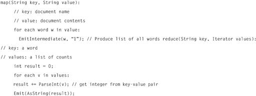
The function EmitIntermediate used in the Map function emits each word in the document and the value one. Then the Reduce function sums all the values per word for each document using ParseInt() to get the number of occurrences per word in all documents. The MapReduce runtime environment schedules map tasks and reduce tasks to the servers of a WSC.
At this extreme scale, which requires innovation in power distribution, cooling, monitoring, and operations, the WSC is a modern descendant of the 1970s supercomputers—making Seymour Cray the godfather of today’s WSC architects. His extreme computers handled computations that could be done nowhere else, but were so expensive that only a few companies could afford them. This time the target is providing information technology for the world instead of high performance computing for scientists and engineers. Hence, WSCs surely play a more important societal role today than Cray’s supercomputers did in the past.
While they share some common goals with servers, WSCs have three major distinctions:
1. Ample, easy parallelism: A concern for a server architect is whether the applications in the targeted marketplace have enough parallelism to justify the amount of parallel hardware and whether the cost is too high for sufficient communication hardware to exploit this parallelism. A WSC architect has no such concern. First, batch applications like MapReduce benefit from the large number of independent data sets that need independent processing, such as billions of Web pages from a Web crawl. Second, interactive Internet service applications, also known as Software as a Service (SaaS), can benefit from millions of independent users of interactive Internet services. Reads and writes are rarely dependent in SaaS, so SaaS rarely needs to synchronize. For example, search uses a read-only index and email is normally reading and writing independent information. We call this type of easy parallelism Request-Level Parallelism, as many independent efforts can proceed in parallel naturally with little need for communication or synchronization.
software as a service (SaaS)
Rather than selling software that is installed and run on customers’ own computers, software is run at a remote site and made available over the Internet typically via a Web interface to customers. SaaS customers are charged based on use versus on ownership.
2. Operational Costs Count: Traditionally, server architects design their systems for peak performance within a cost budget and worry about energy only to make sure they don’t exceed the cooling capacity of their enclosure. They usually ignored operational costs of a server, assuming that they pale in comparison to purchase costs. WSC have longer lifetimes—the building and electrical and cooling infrastructure are often amortized over 10 or more years—so the operational costs add up: energy, power distribution, and cooling represent more than 30% of the costs of a WSC over 10 years.
3. Scale and the Opportunities/Problems Associated with Scale: To construct a single WSC, you must purchase 100,000 servers along with the supporting infrastructure, which means volume discounts. Hence, WSCs are so massive internally that you get economy of scale even if there are not many WSCs. These economies of scale led to cloud computing, as the lower per unit costs of a WSC meant that cloud companies could rent servers at a profitable rate and still be below what it costs outsiders to do it themselves. The flip side of the economic opportunity of scale is the need to cope with the failure frequency of scale. Even if a server had a Mean Time To Failure of an amazing 25 years (200,000 hours), the WSC architect would need to design for 5 server failures every day. Section 5.15 mentioned annualized disk failure rate (AFR) was measured at Google at 2% to 4%. If there were 4 disks per server and their annual failure rate was 2%, the WSC architect should expect to see one disk fail every hour. Thus, fault tolerance is even more important for the WSC architect than the server architect.
The economies of scale uncovered by WSC have realized the long dreamed of goal of computing as a utility. Cloud computing means anyone anywhere with good ideas, a business model, and a credit card can tap thousands of servers to deliver their vision almost instantly around the world. Of course, there are important obstacles that could limit the growth of cloud computing—such as security, privacy, standards, and the rate of growth of Internet bandwidth—but we foresee them being addressed so that WSCs and cloud computing can flourish.
To put the growth rate of cloud computing into perspective, in 2012 Amazon Web Services announced that it adds enough new server capacity every day to support all of Amazon’s global infrastructure as of 2003, when Amazon was a $5.2Bn annual revenue enterprise with 6000 employees.
Now that we understand the importance of message-passing multiprocessors, especially for cloud computing, we next cover ways to connect the nodes of a WSC together. Thanks to Moore’s Law and the increasing number of cores per chip, we now need networks inside a chip as well, so these topologies are important in the small as well as in the large.
Elaboration
The MapReduce framework shuffles and sorts the key-value pairs at the end of the Map phase to produce groups that all share the same key. These groups are then passed to the Reduce phase.
Elaboration
Another form of large scale computing is grid computing, where the computers are spread across large areas, and then the programs that run across them must communicate via long haul networks. The most popular and unique form of grid computing was pioneered by the SETI@home project. As millions of PCs are idle at any one time doing nothing useful, they could be harvested and put to good uses if someone developed software that could run on those computers and then gave each PC an independent piece of the problem to work on. The first example was the Search for ExtraTerrestrial Intelligence (SETI), which was launched at UC Berkeley in 1999. Over 5 million computer users in more than 200 countries have signed up for SETI@home, with more than 50% outside the US. By the end of 2011, the average performance of the SETI@home grid was 3.5 PetaFLOPS.
Check Yourself
1. True or false: Like SMPs, message-passing computers rely on locks for synchronization.
2. True or false: Clusters have separate memories and thus need many copies of the operating system.
6.8 Introduction to Multiprocessor Network Topologies
Multicore chips require on-chip networks to connect cores together, and clusters require local area networks to connect servers together. This section reviews the pros and cons of different interconnection network topologies.
Network costs include the number of switches, the number of links on a switch to connect to the network, the width (number of bits) per link, and length of the links when the network is mapped into silicon. For example, some cores or servers may be adjacent and others may be on the other side of the chip or the other side of the datacenter. Network performance is multifaceted as well. It includes the latency on an unloaded network to send and receive a message, the throughput in terms of the maximum number of messages that can be transmitted in a given time period, delays caused by contention for a portion of the network, and variable performance depending on the pattern of communication. Another obligation of the network may be fault tolerance, since systems may be required to operate in the presence of broken components. Finally, in this era of energy-limited systems, the energy efficiency of different organizations may trump other concerns.
Networks are normally drawn as graphs, with each edge of the graph representing a link of the communication network. In the figures in this section, the processor-memory node is shown as a black square and the switch is shown as a colored circle. We assume here that all links are bidirectional; that is, information can flow in either direction. All networks consist of switches whose links go to processor-memory nodes and to other switches. The first network connects a sequence of nodes together:
![]()
This topology is called a ring. Since some nodes are not directly connected, some messages will have to hop along intermediate nodes until they arrive at the final destination.
Unlike a bus—a shared set of wires that allows broadcasting to all connected devices—a ring is capable of many simultaneous transfers.
Because there are numerous topologies to choose from, performance metrics are needed to distinguish these designs. Two are popular. The first is total network bandwidth, which is the bandwidth of each link multiplied by the number of links. This represents the peak bandwidth. For the ring network above, with P processors, the total network bandwidth would be P times the bandwidth of one link; the total network bandwidth of a bus is just the bandwidth of that bus.
network bandwidth
Informally, the peak transfer rate of a network; can refer to the speed of a single link or the collective transfer rate of all links in the network.
To balance this best bandwidth case, we include another metric that is closer to the worst case: the bisection bandwidth. This metric is calculated by dividing the machine into two halves. Then you sum the bandwidth of the links that cross that imaginary dividing line. The bisection bandwidth of a ring is two times the link bandwidth. It is one times the link bandwidth for the bus. If a single link is as fast as the bus, the ring is only twice as fast as a bus in the worst case, but it is P times faster in the best case.
bisection bandwidth
The bandwidth between two equal parts of a multiprocessor. This measure is for a worst case split of the multiprocessor.
Since some network topologies are not symmetric, the question arises of where to draw the imaginary line when bisecting the machine. Bisection bandwidth is a worst-case metric, so the answer is to choose the division that yields the most pessimistic network performance. Stated alternatively, calculate all possible bisection bandwidths and pick the smallest. We take this pessimistic view because parallel programs are often limited by the weakest link in the communication chain.
At the other extreme from a ring is a fully connected network, where every processor has a bidirectional link to every other processor. For fully connected networks, the total network bandwidth is P×(P−1)/2, and the bisection bandwidth is (P/2)2.
fully connected network
A network that connects processor-memory nodes by supplying a dedicated communication link between every node.
The tremendous improvement in performance of fully connected networks is offset by the tremendous increase in cost. This consequence inspires engineers to invent new topologies that are between the cost of rings and the performance of fully connected networks. The evaluation of success depends in large part on the nature of the communication in the workload of parallel programs run on the computer.
The number of different topologies that have been discussed in publications would be difficult to count, but only a few have been used in commercial parallel processors. Figure 6.14 illustrates two of the popular topologies.
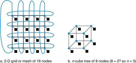
FIGURE 6.14 Network topologies that have appeared in commercial parallel processors.
The colored circles represent switches and the black squares represent processor-memory nodes. Even though a switch has many links, generally only one goes to the processor. The Boolean n-cube topology is an n-dimensional interconnect with 2n nodes, requiring n links per switch (plus one for the processor) and thus n nearest-neighbor nodes. Frequently, these basic topologies have been supplemented with extra arcs to improve performance and reliability.
An alternative to placing a processor at every node in a network is to leave only the switch at some of these nodes. The switches are smaller than processor-memory-switch nodes, and thus may be packed more densely, thereby lessening distance and increasing performance. Such networks are frequently called multistage networks to reflect the multiple steps that a message may travel. Types of multistage networks are as numerous as single-stage networks; Figure 6.15 illustrates two of the popular multistage organizations. A fully connected or crossbar network allows any node to communicate with any other node in one pass through the network. An Omega network uses less hardware than the crossbar network (2n log2n versus n2 switches), but contention can occur between messages, depending on the pattern of communication. For example, the Omega network in Figure 6.15 cannot send a message from P0 to P6 at the same time that it sends a message from P1 to P4.
multistage network
A network that supplies a small switch at each node.
crossbar network
A network that allows any node to communicate with any other node in one pass through the network.
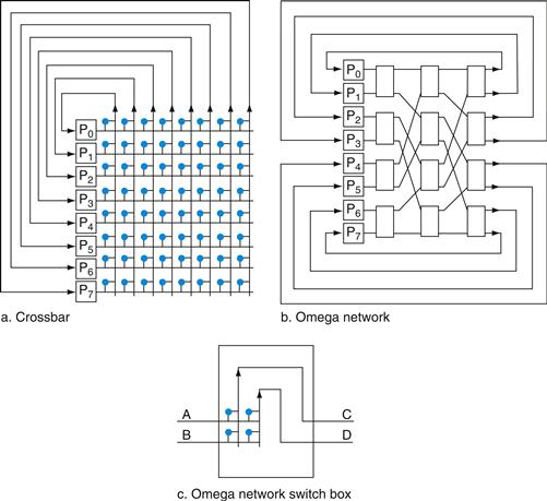
FIGURE 6.15 Popular multistage network topologies for eight nodes.
The switches in these drawings are simpler than in earlier drawings because the links are unidirectional; data comes in at the left and exits out the right link. The switch box in c can pass A to C and B to D or B to C and A to D. The crossbar uses n2 switches, where n is the number of processors, while the Omega network uses 2n log2n of the large switch boxes, each of which is logically composed of four of the smaller switches. In this case, the crossbar uses 64 switches versus 12 switch boxes, or 48 switches, in the Omega network. The crossbar, however, can support any combination of messages between processors, while the Omega network cannot.
Implementing Network Topologies
This simple analysis of all the networks in this section ignores important practical considerations in the construction of a network. The distance of each link affects the cost of communicating at a high clock rate—generally, the longer the distance, the more expensive it is to run at a high clock rate. Shorter distances also make it easier to assign more wires to the link, as the power to drive many wires is less if the wires are short. Shorter wires are also cheaper than longer wires. Another practical limitation is that the three-dimensional drawings must be mapped onto chips that are essentially two-dimensional media. The final concern is energy. Energy concerns may force multicore chips to rely on simple grid topologies, for example. The bottom line is that topologies that appear elegant when sketched on the blackboard may be impractical when constructed in silicon or in a datacenter.
Now that we understand the importance of clusters and have seen topologies that we can follow to connect them together, we next look at the hardware and software of the interface of the network to the processor.
Check Yourself
True or false: For a ring with P nodes, the ratio of the total network bandwidth to the bisection bandwidth is P/2.
 Communicating to the Outside World: Cluster Networking
This online section describes the networking hardware and software used to connect the nodes of a cluster together. The example is 10 gigabit/second Ethernet connected to the computer using Peripheral Component Interconnect Express (PCIe). It shows both software and hardware optimizations how to improve network performance, including zero copy messaging, user space communication, using polling instead of I/O interrupts, and hardware calculation of checksums. While the example is networking, the techniques in this section apply to storage controllers and other I/O devices as well.
After covering the performance of network at a low level of detail in this online section, the next section shows how to benchmark multiprocessors of all kinds with much higher-level programs.
6.10 Multiprocessor Benchmarks and Performance Models
As we saw in Chapter 1, benchmarking systems is always a sensitive topic, because it is a highly visible way to try to determine which system is better. The results affect not only the sales of commercial systems, but also the reputation of the designers of those systems. Hence, all participants want to win the competition, but they also want to be sure that if someone else wins, they deserve to win because they have a genuinely better system. This desire leads to rules to ensure that the benchmark results are not simply engineering tricks for that benchmark, but are instead advances that improve performance of real applications.
To avoid possible tricks, a typical rule is that you can’t change the benchmark. The source code and data sets are fixed, and there is a single proper answer. Any deviation from those rules makes the results invalid.
Many multiprocessor benchmarks follow these traditions. A common exception is to be able to increase the size of the problem so that you can run the benchmark on systems with a widely different number of processors. That is, many benchmarks allow weak scaling rather than require strong scaling, even though you must take care when comparing results for programs running different problem sizes.
Figure 6.16 gives a summary of several parallel benchmarks, also described below:
■ Linpack is a collection of linear algebra routines, and the routines for performing Gaussian elimination constitute what is known as the Linpack benchmark. The DGEMM routine in the example on page 215 represents a small fraction of the source code of the Linpack benchmark, but it accounts for most of the execution time for the benchmark. It allows weak scaling, letting the user pick any size problem. Moreover, it allows the user to rewrite Linpack in almost any form and in any language, as long as it computes the proper result and performs the same number of floating point operations for a given problem size. Twice a year, the 500 computers with the fastest Linpack performance are published at www.top500.org. The first on this list is considered by the press to be the world’s fastest computer.
■ SPECrate is a throughput metric based on the SPEC CPU benchmarks, such as SPEC CPU 2006 (see Chapter 1). Rather than report performance of the individual programs, SPECrate runs many copies of the program simultaneously. Thus, it measures task-level parallelism, as there is no communication between the tasks. You can run as many copies of the programs as you want, so this is again a form of weak scaling.
■ SPLASH and SPLASH 2 (Stanford Parallel Applications for Shared Memory) were efforts by researchers at Stanford University in the 1990s to put together a parallel benchmark suite similar in goals to the SPEC CPU benchmark suite. It includes both kernels and applications, including many from the high-performance computing community. This benchmark requires strong scaling, although it comes with two data sets.
■ The NAS (NASA Advanced Supercomputing) parallel benchmarks were another attempt from the 1990s to benchmark multiprocessors. Taken from computational fluid dynamics, they consist of five kernels. They allow weak scaling by defining a few data sets. Like Linpack, these benchmarks can be rewritten, but the rules require that the programming language can only be C or Fortran.
■ The recent PARSEC (Princeton Application Repository for Shared Memory Computers) benchmark suite consists of multithreaded programs that use Pthreads (POSIX threads) and OpenMP (Open MultiProcessing; see Section 6.5). They focus on emerging computational domains and consist of nine applications and three kernels. Eight rely on data parallelism, three rely on pipelined parallelism, and one on unstructured parallelism.
■ On the cloud front, the goal of the Yahoo! Cloud Serving Benchmark (YCSB) is to compare performance of cloud data services. It offers a framework that makes it easy for a client to benchmark new data services, using Cassandra and HBase as representative examples. [Cooper, 2010]
Pthreads
A UNIX API for creating and manipulating threads. It is structured as a library.
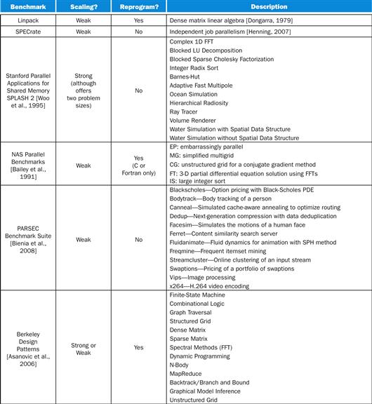
FIGURE 6.16 Examples of parallel benchmarks.
The downside of such traditional restrictions to benchmarks is that innovation is chiefly limited to the architecture and compiler. Better data structures, algorithms, programming languages, and so on often cannot be used, since that would give a misleading result. The system could win because of, say, the algorithm, and not because of the hardware or the compiler.
While these guidelines are understandable when the foundations of computing are relatively stable—as they were in the 1990s and the first half of this decade—they are undesirable during a programming revolution. For this revolution to succeed, we need to encourage innovation at all levels.
Researchers at the University of California at Berkeley have advocated one approach. They identified 13 design patterns that they claim will be part of applications of the future. Frameworks or kernels implement these design patterns. Examples are sparse matrices, structured grids, finite-state machines, map reduce, and graph traversal. By keeping the definitions at a high level, they hope to encourage innovations at any level of the system. Thus, the system with the fastest sparse matrix solver is welcome to use any data structure, algorithm, and programming language, in addition to novel architectures and compilers.
Performance Models
A topic related to benchmarks is performance models. As we have seen with the increasing architectural diversity in this chapter—multithreading, SIMD, GPUs—it would be especially helpful if we had a simple model that offered insights into the performance of different architectures. It need not be perfect, just insightful.
The 3Cs for cache performance from Chapter 5 is an example performance model. It is not a perfect performance model, since it ignores potentially important factors like block size, block allocation policy, and block replacement policy. Moreover, it has quirks. For example, a miss can be ascribed due to capacity in one design and to a conflict miss in another cache of the same size. Yet 3Cs model has been popular for 25 years, because it offers insight into the behavior of programs, helping both architects and programmers improve their creations based on insights from that model.
To find such a model for parallel computers, let’s start with small kernels, like those from the 13 Berkeley design patterns in Figure 6.16. While there are versions with different data types for these kernels, floating point is popular in several implementations. Hence, peak floating-point performance is a limit on the speed of such kernels on a given computer. For multicore chips, peak floating-point performance is the collective peak performance of all the cores on the chip. If there were multiple microprocessors in the system, you would multiply the peak per chip by the total number of chips.
The demands on the memory system can be estimated by dividing this peak floating-point performance by the average number of floating-point operations per byte accessed:
![]()
The ratio of floating-point operations per byte of memory accessed is called the arithmetic intensity. It can be calculated by taking the total number of floating-point operations for a program divided by the total number of data bytes transferred to main memory during program execution. Figure 6.17 shows the arithmetic intensity of several of the Berkeley design patterns from Figure 6.16.
arithmetic intensity
The ratio of floating-point operations in a program to the number of data bytes accessed by a program from main memory.
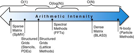
FIGURE 6.17 Arithmetic intensity, specified as the number of float-point operations to run the program divided by the number of bytes accessed in main memory [Williams, Waterman, and Patterson, 2009].
Some kernels have an arithmetic intensity that scales with problem size, such as Dense Matrix, but there are many kernels with arithmetic intensities independent of problem size. For kernels in this former case, weak scaling can lead to different results, since it puts much less demand on the memory system.
The Roofline Model
This simple model ties floating-point performance, arithmetic intensity, and memory performance together in a two-dimensional graph [Williams, Waterman, and Patterson, 2009]. Peak floating-point performance can be found using the hardware specifications mentioned above. The working sets of the kernels we consider here do not fit in on-chip caches, so peak memory performance may be defined by the memory system behind the caches. One way to find the peak memory performance is the Stream benchmark. (See the Elaboration on page 381 in Chapter 5).
Figure 6.18 shows the model, which is done once for a computer, not for each kernel. The vertical Y-axis is achievable floating-point performance from 0.5 to 64.0 GFLOPs/second. The horizontal X-axis is arithmetic intensity, varying from 1/8 FLOPs/DRAM byte accessed to 16 FLOPs/DRAM byte accessed. Note that the graph is a log-log scale.
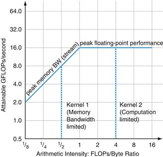
FIGURE 6.18 Roofline Model [Williams, Waterman, and Patterson, 2009].
This example has a peak floating-point performance of 16 GFLOPS/sec and a peak memory bandwidth of 16 GB/sec from the Stream benchmark. (Since Stream is actually four measurements, this line is the average of the four.) The dotted vertical line in color on the left represents Kernel 1, which has an arithmetic intensity of 0.5 FLOPs/byte. It is limited by memory bandwidth to no more than 8 GFLOPS/sec on this Opteron X2. The dotted vertical line to the right represents Kernel 2, which has an arithmetic intensity of 4 FLOPs/byte. It is limited only computationally to 16 GFLOPS/s. (This data is based on the AMD Opteron X2 (Revision F) using dual cores running at 2 GHz in a dual socket system.)
For a given kernel, we can find a point on the X-axis based on its arithmetic intensity. If we draw a vertical line through that point, the performance of the kernel on that computer must lie somewhere along that line. We can plot a horizontal line showing peak floating-point performance of the computer. Obviously, the actual floating-point performance can be no higher than the horizontal line, since that is a hardware limit.
How could we plot the peak memory performance, which is measured in bytes/second? Since the X-axis is FLOPs/byte and the Y-axis FLOPs/second, bytes/second is just a diagonal line at a 45-degree angle in this figure. Hence, we can plot a third line that gives the maximum floating-point performance that the memory system of that computer can support for a given arithmetic intensity. We can express the limits as a formula to plot the line in the graph in Figure 6.18:
![]()
The horizontal and diagonal lines give this simple model its name and indicate its value. The “roofline” sets an upper bound on performance of a kernel depending on its arithmetic intensity. Given a roofline of a computer, you can apply it repeatedly, since it doesn’t vary by kernel.
If we think of arithmetic intensity as a pole that hits the roof, either it hits the slanted part of the roof, which means performance is ultimately limited by memory bandwidth, or it hits the flat part of the roof, which means performance is computationally limited. In Figure 6.18, kernel 1 is an example of the former, and kernel 2 is an example of the latter.
Note that the “ridge point,” where the diagonal and horizontal roofs meet, offers an interesting insight into the computer. If it is far to the right, then only kernels with very high arithmetic intensity can achieve the maximum performance of that computer. If it is far to the left, then almost any kernel can potentially hit the maximum performance.
Comparing Two Generations of Opterons
The AMD Opteron X4 (Barcelona) with four cores is the successor to the Opteron X2 with two cores. To simplify board design, they use the same socket. Hence, they have the same DRAM channels and thus the same peak memory bandwidth. In addition to doubling the number of cores, the Opteron X4 also has twice the peak floating-point performance per core: Opteron X4 cores can issue two floating-point SSE2 instructions per clock cycle, while Opteron X2 cores issue at most one. As the two systems we’re comparing have similar clock rates—2.2 GHz for Opteron X2 versus 2.3 GHz for Opteron X4—the Opteron X4 has about four times the peak floating-point performance of the Opteron X2 with the same DRAM bandwidth. The Opteron X4 also has a 2MB L3 cache, which is not found in the Opteron X2.
In Figure 6.19 the roofline models for both systems are compared. As we would expect, the ridge point moves to the right, from 1 in the Opteron X2 to 5 in the Opteron X4. Hence, to see a performance gain in the next generation, kernels need an arithmetic intensity higher than 1, or their working sets must fit in the caches of the Opteron X4.
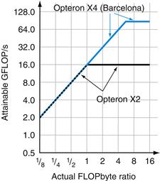
FIGURE 6.19 Roofline models of two generations of Opterons.
The Opteron X2 roofline, which is the same as in Figure 6.18, is in black, and the Opteron X4 roofline is in color. The bigger ridge point of Opteron X4 means that kernels that were computationally bound on the Opteron X2 could be memory-performance bound on the Opteron X4.
The roofline model gives an upper bound to performance. Suppose your program is far below that bound. What optimizations should you perform, and in what order?
To reduce computational bottlenecks, the following two optimizations can help almost any kernel:
1. Floating-point operation mix. Peak floating-point performance for a computer typically requires an equal number of nearly simultaneous additions and multiplications. That balance is necessary either because the computer supports a fused multiply-add instruction (see the Elaboration on page 220 in Chapter 3) or because the floating-point unit has an equal number of floating-point adders and floating-point multipliers. The best performance also requires that a significant fraction of the instruction mix is floating-point operations and not integer instructions.
2. Improve instruction-level parallelism and apply SIMD. For modern architectures, the highest performance comes when fetching, executing, and committing three to four instructions per clock cycle (see Section 4.10). The goal for this step is to improve the code from the compiler to increase ILP. One way is by unrolling loops, as we saw in Section 4.12. For the x86 architectures, a single AVX instruction can operate on four double precision operands, so they should be used whenever possible (see Sections 3.7 and 3.8).
To reduce memory bottlenecks, the following two optimizations can help:
1. Software prefetching. Usually the highest performance requires keeping many memory operations in flight, which is easier to do by performing predicting accesses via software prefetch instructions rather than waiting until the data is required by the computation.

2. Memory affinity. Microprocessors today include a memory controller on the same chip with the microprocessor, which improves performance of the memory hierarchy. If the system has multiple chips, this means that some addresses go to the DRAM that is local to one chip, and the rest require accesses over the chip interconnect to access the DRAM that is local to another chip. This split results in nonuniform memory accesses, which we described in Section 6.5. Accessing memory through another chip lowers performance. This second optimization tries to allocate data and the threads tasked to operate on that data to the same memory-processor pair, so that the processors rarely have to access the memory of the other chips.
The roofline model can help decide which of these two optimizations to perform and the order in which to perform them. We can think of each of these optimizations as a “ceiling” below the appropriate roofline, meaning that you cannot break through a ceiling without performing the associated optimization.
The computational roofline can be found from the manuals, and the memory roofline can be found from running the Stream benchmark. The computational ceilings, such as floating-point balance, can also come from the manuals for that computer. A memory ceiling, such as memory affinity, requires running experiments on each computer to determine the gap between them. The good news is that this process only need be done once per computer, for once someone characterizes a computer’s ceilings, everyone can use the results to prioritize their optimizations for that computer.
Figure 6.20 adds ceilings to the roofline model in Figure 6.18, showing the computational ceilings in the top graph and the memory bandwidth ceilings on the bottom graph. Although the higher ceilings are not labeled with both optimizations, they are implied in this figure; to break through the highest ceiling, you need to have already broken through all the ones below.
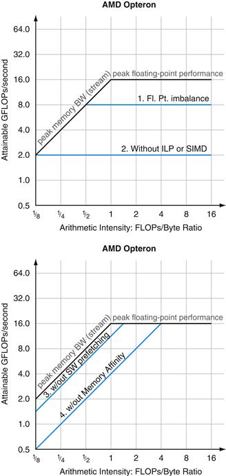
FIGURE 6.20 Roofline model with ceilings.
The top graph shows the computational “ceilings” of 8 GFLOPs/sec if the floating-point operation mix is imbalanced and 2 GFLOPs/sec if the optimizations to increase ILP and SIMD are also missing. The bottom graph shows the memory bandwidth ceilings of 11 GB/sec without software prefetching and 4.8 GB/sec if memory affinity optimizations are also missing.
The width of the gap between the ceiling and the next higher limit is the reward for trying that optimization. Thus, Figure 6.20 suggests that optimization 2, which improves ILP, has a large benefit for improving computation on that computer, and optimization 4, which improves memory affinity, has a large benefit for improving memory bandwidth on that computer.
Figure 6.21 combines the ceilings of Figure 6.20 into a single graph. The arithmetic intensity of a kernel determines the optimization region, which in turn suggests which optimizations to try. Note that the computational optimizations and the memory bandwidth optimizations overlap for much of the arithmetic intensity. Three regions are shaded differently in Figure 6.21 to indicate the different optimization strategies. For example, Kernel 2 falls in the blue trapezoid on the right, which suggests working only on the computational optimizations. Kernel 1 falls in the blue-gray parallelogram in the middle, which suggests trying both types of optimizations. Moreover, it suggests starting with optimizations 2 and 4. Note that the Kernel 1 vertical lines fall below the floating-point imbalance optimization, so optimization 1 may be unnecessary. If a kernel fell in the gray triangle on the lower left, it would suggest trying just memory optimizations.
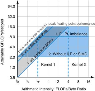
FIGURE 6.21 Roofline model with ceilings, overlapping areas shaded, and the two kernels from Figure 6.18.
Kernels whose arithmetic intensity land in the blue trapezoid on the right should focus on computation optimizations, and kernels whose arithmetic intensity land in the gray triangle in the lower left should focus on memory bandwidth optimizations. Those that land in the blue-gray parallelogram in the middle need to worry about both. As Kernel 1 falls in the parallelogram in the middle, try optimizing ILP and SIMD, memory affinity, and software prefetching. Kernel 2 falls in the trapezoid on the right, so try optimizing ILP and SIMD and the balance of floating-point operations.
Thus far, we have been assuming that the arithmetic intensity is fixed, but that is not really the case. First, there are kernels where the arithmetic intensity increases with problem size, such as for Dense Matrix and N-body problems (see Figure 6.17). Indeed, this can be a reason that programmers have more success with weak scaling than with strong scaling. Second, the effectiveness of the memory hierarchy affects the number of accesses that go to memory, so optimizations that improve cache performance also improve arithmetic intensity. One example is improving temporal locality by unrolling loops and then grouping together statements with similar addresses. Many computers have special cache instructions that allocate data in a cache but do not first fill the data from memory at that address, since it will soon be over-written. Both these optimizations reduce memory traffic, thereby moving the arithmetic intensity pole to the right by a factor of, say, 1.5. This shift right could put the kernel in a different optimization region.
While the examples above show how to help programmers improve performance, architects can also use the model to decide where they should optimize hardware to improve performance of the kernels that they think will be important.
The next section uses the roofline model to demonstrate the performance difference between a multicore microprocessor and a GPU and to see whether these differences reflect performance of real programs.
Elaboration
The ceilings are ordered so that lower ceilings are easier to optimize. Clearly, a programmer can optimize in any order, but following this sequence reduces the chances of wasting effort on an optimization that has no benefit due to other constraints. Like the 3Cs model, as long as the roofline model delivers on insights, a model can have assumptions that may prove optimistic. For example, roofline assumes the load is balanced between all processors.
Elaboration
An alternative to the Stream benchmark is to use the raw DRAM bandwidth as the roofline. While the raw bandwidth definitely is a hard upper bound, actual memory performance is often so far from that boundary that it’s not that useful. That is, no program can go close to that bound. The downside to using Stream is that very careful programming may exceed the Stream results, so the memory roofline may not be as hard a limit as the computational roofline. We stick with Stream because few programmers will be able to deliver more memory bandwidth than Stream discovers.
Elaboration
Although the roofline model shown is for multicore processors, it clearly would work for a uniprocessor as well.
Check Yourself
True or false: The main drawback with conventional approaches to benchmarks for parallel computers is that the rules that ensure fairness also slow software innovation.
6.11 Real Stuff: Benchmarking and Rooflines of the Intel Core i7 960 and the NVIDIA Tesla GPU
A group of Intel researchers published a paper [Lee et al., 2010] comparing a quad-core Intel Core i7 960 with multimedia SIMD extensions to the previous generation GPU, the NVIDIA Tesla GTX 280. Figure 6.22 lists the characteristics of the two systems. Both products were purchased in Fall 2009. The Core i7 is in Intel’s 45-nanometer semiconductor technology while the GPU is in TSMC’s 65-nanometer technology. Although it might have been fairer to have a comparison by a neutral party or by both interested parties, the purpose of this section is not to determine how much faster one product is than another, but to try to understand the relative value of features of these two contrasting architecture styles.
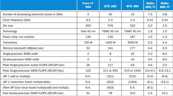
FIGURE 6.22 Intel Core i7-960, NVIDIA GTX 280, and GTX 480 specifications.
The rightmost columns show the ratios of the Tesla GTX 280 and the Fermi GTX 480 to Core i7. Although the case study is between the Tesla 280 and i7, we include the Fermi 480 to show its relationship to the Tesla 280 since it is described in this chapter. Note that these memory bandwidths are higher than in Figure 6.23 because these are DRAM pin bandwidths and those in Figure 6.23 are at the processors as measured by a benchmark program. (From Table 2 in Lee et al. [2010].)
The rooflines of the Core i7 960 and GTX 280 in Figure 6.23 illustrate the differences in the computers. Not only does the GTX 280 have much higher memory bandwidth and double-precision floating-point performance, but also its double-precision ridge point is considerably to the left. The double-precision ridge point is 0.6 for the GTX 280 versus 3.1 for the Core i7. As mentioned above, it is much easier to hit peak computational performance the further the ridge point of the roofline is to the left. For single-precision performance, the ridge point moves far to the right for both computers, so it’s much harder to hit the roof of single-precision performance. Note that the arithmetic intensity of the kernel is based on the bytes that go to main memory, not the bytes that go to cache memory. Thus, as mentioned above, caching can change the arithmetic intensity of a kernel on a particular computer, if most references really go to the cache. Note also that this bandwidth is for unit-stride accesses in both architectures. Real gather-scatter addresses can be slower on the GTX 280 and on the Core i7, as we shall see.
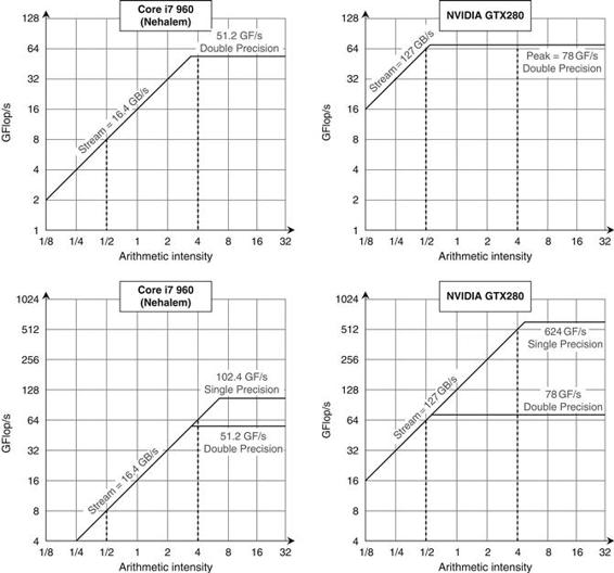
FIGURE 6.23 Roofline model [Williams, Waterman, and Patterson, 2009].
These rooflines show double-precision floating-point performance in the top row and single-precision performance in the bottom row. (The DP FP performance ceiling is also in the bottom row to give perspective.) The Core i7 960 on the left has a peak DP FP performance of 51.2 GFLOP/sec, a SP FP peak of 102.4 GFLOP/sec, and a peak memory bandwidth of 16.4 GBytes/sec. The NVIDIA GTX 280 has a DP FP peak of 78 GFLOP/sec, SP FP peak of 624 GFLOP/sec, and 127 GBytes/sec of memory bandwidth. The dashed vertical line on the left represents an arithmetic intensity of 0.5 FLOP/byte. It is limited by memory bandwidth to no more than 8 DP GFLOP/sec or 8 SP GFLOP/sec on the Core i7. The dashed vertical line to the right has an arithmetic intensity of 4 FLOP/byte. It is limited only computationally to 51.2 DP GFLOP/sec and 102.4 SP GFLOP/sec on the Core i7 and 78 DP GFLOP/sec and 512 DP GFLOP/sec on the GTX 280. To hit the highest computation rate on the Core i7 you need to use all 4 cores and SSE instructions with an equal number of multiplies and adds. For the GTX 280, you need to use fused multiply-add instructions on all multithreaded SIMD processors.
The researchers selected the benchmark programs by analyzing the computational and memory characteristics of four recently proposed benchmark suites and then “formulated the set of throughput computing kernels that capture these characteristics.” Figure 6.24 shows the performance results, with larger numbers meaning faster. The Rooflines help explain the relative performance in this case study.
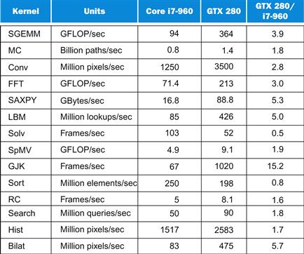
FIGURE 6.24 Raw and relative performance measured for the two platforms.
In this study, SAXPY is just used as a measure of memory bandwidth, so the right unit is GBytes/sec and not GFLOP/sec. (Based on Table 3 in [Lee et al., 2010].)
Given that the raw performance specifications of the GTX 280 vary from 2.5×slower (clock rate) to 7.5×faster (cores per chip) while the performance varies from 2.0×slower (Solv) to 15.2×faster (GJK), the Intel researchers decided to find the reasons for the differences:
■ Memory bandwidth. The GPU has 4.4×the memory bandwidth, which helps explain why LBM and SAXPY run 5.0 and 5.3×faster; their working sets are hundreds of megabytes and hence don’t fit into the Core i7 cache. (So as to access memory intensively, they purposely did not use cache blocking as in Chapter 5.) Hence, the slope of the rooflines explains their performance. SpMV also has a large working set, but it only runs 1.9×faster because the double-precision floating point of the GTX 280 is only 1.5×as faster as the Core i7.
■ Compute bandwidth. Five of the remaining kernels are compute bound: SGEMM, Conv, FFT, MC, and Bilat. The GTX is faster by 3.9, 2.8, 3.0, 1.8, and 5.7×, respectively. The first three of these use single-precision floating-point arithmetic, and GTX 280 single precision is 3 to 6×faster. MC uses double precision, which explains why it’s only 1.8×faster since DP performance is only 1.5×faster. Bilat uses transcendental functions, which the GTX 280 supports directly. The Core i7 spends two-thirds of its time calculating transcendental functions for Bilat, so the GTX 280 is 5.7×faster. This observation helps point out the value of hardware support for operations that occur in your workload: double-precision floating point and perhaps even transcendentals.
■ Cache benefits. Ray casting (RC) is only 1.6×faster on the GTX because cache blocking with the Core i7 caches prevents it from becoming memory bandwidth bound (see Sections 5.4 and 5.14), as it is on GPUs. Cache blocking can help Search, too. If the index trees are small so that they fit in the cache, the Core i7 is twice as fast. Larger index trees make them memory bandwidth bound. Overall, the GTX 280 runs search 1.8×faster. Cache blocking also helps Sort. While most programmers wouldn’t run Sort on a SIMD processor, it can be written with a 1-bit Sort primitive called split. However, the split algorithm executes many more instructions than a scalar sort does. As a result, the Core i7 runs 1.25×as fast as the GTX 280. Note that caches also help other kernels on the Core i7, since cache blocking allows SGEMM, FFT, and SpMV to become compute bound. This observation re-emphasizes the importance of cache blocking optimizations in Chapter 5.
■ Gather-Scatter. The multimedia SIMD extensions are of little help if the data are scattered throughout main memory; optimal performance comes only when accesses are to data are aligned on 16-byte boundaries. Thus, GJK gets little benefit from SIMD on the Core i7. As mentioned above, GPUs offer gather-scatter addressing that is found in a vector architecture but omitted from most SIMD extensions. The memory controller even batches accesses to the same DRAM page together (see Section 5.2). This combination means the GTX 280 runs GJK a startling 15.2×as fast as the Core i7, which is larger than any single physical parameter in Figure 6.22. This observation reinforces the importance of gather-scatter to vector and GPU architectures that is missing from SIMD extensions.
■ Synchronization. The performance of synchronization is limited by atomic updates, which are responsible for 28% of the total runtime on the Core i7 despite its having a hardware fetch-and-increment instruction. Thus, Hist is only 1.7×faster on the GTX 280. Solv solves a batch of independent constraints in a small amount of computation followed by barrier synchronization. The Core i7 benefits from the atomic instructions and a memory consistency model that ensures the right results even if not all previous accesses to memory hierarchy have completed. Without the memory consistency model, the GTX 280 version launches some batches from the system processor, which leads to the GTX 280 running 0.5×as fast as the Core i7. This observation points out how synchronization performance can be important for some data parallel problems.
It is striking how often weaknesses in the Tesla GTX 280 that were uncovered by kernels selected by Intel researchers were already being addressed in the successor architecture to Tesla: Fermi has faster double-precision floating-point performance, faster atomic operations, and caches. It was also interesting that the gather-scatter support of vector architectures that predate the SIMD instructions by decades was so important to the effective usefulness of these SIMD extensions, which some had predicted before the comparison. The Intel researchers noted that 6 of the 14 kernels would exploit SIMD better with more efficient gather-scatter support on the Core i7. This study certainly establishes the importance of cache blocking as well.
Now that we seen a wide range of results of benchmarking different multiprocessors, let’s return to our DGEMM example to see in detail how much we have to change the C code to exploit multiple processors.
6.12 Going Faster: Multiple Processors and Matrix Multiply
This section is the final and largest step in our incremental performance journey of adapting DGEMM to the underlying hardware of the Intel Core i7 (Sandy Bridge). Each Core i7 has 8 cores, and the computer we have been using has 2 Core i7s. Thus, we have 16 cores on which to run DGEMM.
Figure 6.25 shows the OpenMP version of DGEMM that utilizes those cores. Note that line 30 is the single line added to Figure 5.48 to make this code run on multiple processors: an OpenMP pragma that tells the compiler to use multiple threads in the outermost for loop. It tells the computer to spread the work of the outermost loop across all the threads.
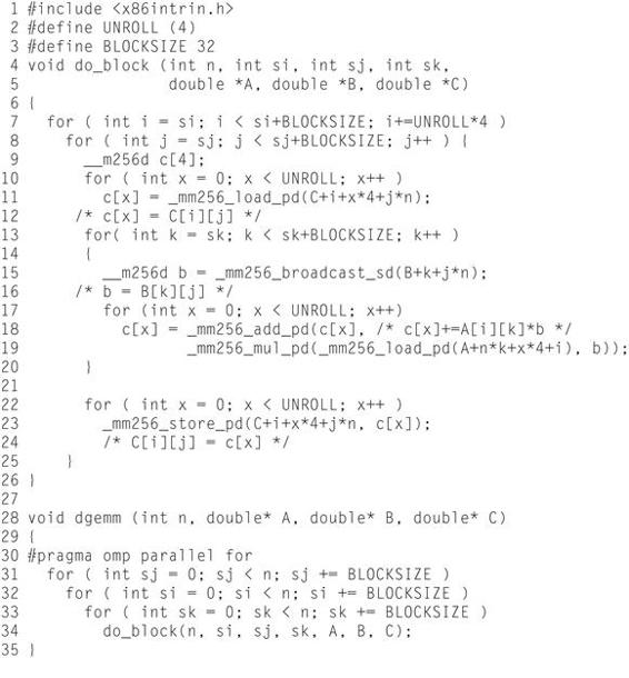
FIGURE 6.25 OpenMP version of DGEMM from Figure 5.48.
Line 30 is the only OpenMP code, making the outermost for loop operate in parallel. This line is the only difference from Figure 5.48.
Figure 6.26 plots a classic multiprocessor speedup graph, showing the performance improvement versus a single thread as the number of threads increase. This graph makes it easy to see the challenges of strong scaling versus weak scaling. When everything fits in the first level data cache, as is the case for 32×32 matrices, adding threads actually hurts performance. The 16-threaded version of DGEMM is almost half as fast as the single-threaded version in this case. In contrast, the two largest matrices get a 14×speedup from 16 threads, and hence the classic two “up and to the right” lines in Figure 6.26.
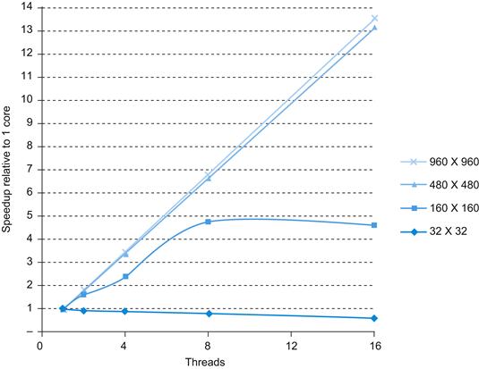
FIGURE 6.26 Performance improvements relative to a single thread as the number of threads increase.
The most honest way to present such graphs is to make performance relative to the best version of a single processor program, which we did. This plot is relative to the performance of the code in Figure 5.48 without including OpenMP pragmas.
Figure 6.27 shows the absolute performance increase as we increase the number of threads from 1 to 16. DGEMM operates now operates at 174 GLOPS for 960×960 matrices. As our unoptimized C version of DGEMM in Figure 3.21 ran this code at just 0.8 GFOPS, the optimizations in Chapters 3 to 6 that tailor the code to the underlying hardware result in a speedup of over 200 times!
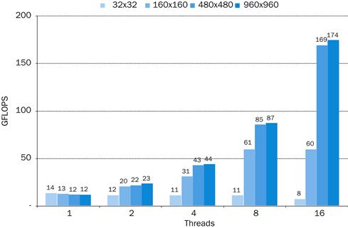
FIGURE 6.27 DGEMM performance versus the number of threads for four matrix sizes.
The performance improvement compared unoptimized code in Figure 3.21 for the 960×960 matrix with 16 threads is an astounding 212 times faster!
Next up is our warnings of the fallacies and pitfalls of multiprocessing. The computer architecture graveyard is filled with parallel processing projects that have ignored them.
Elaboration
These results are with Turbo mode turned off. We are using a dual chip system in this system, so not surprisingly, we can get the full Turbo speedup (3.3/2.6=1.27) with either 1 thread (only 1 core on one of the chips) or 2 threads (1 core per chip). As we increase the number of threads and hence the number of active cores, the benefit of Turbo mode decreases, as there is less of the power budget to spend on the active cores. For 4 threads the average Turbo speedup is 1.23, for 8 it is 1.13, and for 16 it is 1.11.
Elaboration
Although the Sandy Bridge supports two hardware threads per core, we do not get more performance from 32 threads. The reason is that a single AVX hardware is shared between the two threads multiplexed onto one core, so assigning two threads per core actually hurts performance due to the multiplexing overhead.
6.13 Fallacies and Pitfalls
For over a decade prophets have voiced the contention that the organization of a single computer has reached its limits and that truly significant advances can be made only by interconnection of a multiplicity of computers in such a manner as to permit cooperative solution. …Demonstration is made of the continued validity of the single processor approach …
Gene Amdahl, “Validity of the single processor approach to achieving large scale computing capabilities,” Spring Joint Computer Conference, 1967
The many assaults on parallel processing have uncovered numerous fallacies and pitfalls. We cover four here.
Fallacy: Amdahl’s Law doesn’t apply to parallel computers.
In 1987, the head of a research organization claimed that a multiprocessor machine had broken Amdahl’s Law. To try to understand the basis of the media reports, let’s see the quote that gave us Amdahl’s Law [1967, p. 483]:
A fairly obvious conclusion which can be drawn at this point is that the effort expended on achieving high parallel processing rates is wasted unless it is accompanied by achievements in sequential processing rates of very nearly the same magnitude.
This statement must still be true; the neglected portion of the program must limit performance. One interpretation of the law leads to the following lemma: portions of every program must be sequential, so there must be an economic upper bound to the number of processors—say, 100. By showing linear speedup with 1000 processors, this lemma is disproved; hence the claim that Amdahl’s Law was broken.
The approach of the researchers was just to use weak scaling: rather than going 1000 times faster on the same data set, they computed 1000 times more work in comparable time. For their algorithm, the sequential portion of the program was constant, independent of the size of the input, and the rest was fully parallel—hence, linear speedup with 1000 processors.
Amdahl’s Law obviously applies to parallel processors. What this research does point out is that one of the main uses of faster computers is to run larger problems. Just be sure that users really care about those problems versus being a justification to buying an expensive computer by finding a problem that just keeps lots of processors busy.
Fallacy: Peak performance tracks observed performance.
The supercomputer industry once used this metric in marketing, and the fallacy is exacerbated with parallel machines. Not only are marketers using the nearly unattainable peak performance of a uniprocessor node, but also they are then multiplying it by the total number of processors, assuming perfect speedup! Amdahl’s Law suggests how difficult it is to reach either peak; multiplying the two together multiplies the sins. The roofline model helps put peak performance in perspective.
Pitfall: Not developing the software to take advantage of, or optimize for, a multiprocessor architecture.
There is a long history of parallel software lagging behind on parallel hardware, possibly because the software problems are much harder. We give one example to show the subtlety of the issues, but there are many examples we could choose!
One frequently encountered problem occurs when software designed for a uniprocessor is adapted to a multiprocessor environment. For example, the Silicon Graphics operating system originally protected the page table with a single lock, assuming that page allocation is infrequent. In a uniprocessor, this does not represent a performance problem. In a multiprocessor, it can become a major performance bottleneck for some programs. Consider a program that uses a large number of pages that are initialized at start-up, which UNIX does for statically allocated pages. Suppose the program is parallelized so that multiple processes allocate the pages. Because page allocation requires the use of the page table, which is locked whenever it is in use, even an OS kernel that allows multiple threads in the OS will be serialized if the processes all try to allocate their pages at once (which is exactly what we might expect at initialization time!).
This page table serialization eliminates parallelism in initialization and has significant impact on overall parallel performance. This performance bottleneck persists even for task-level parallelism. For example, suppose we split the parallel processing program apart into separate jobs and run them, one job per processor, so that there is no sharing between the jobs. (This is exactly what one user did, since he reasonably believed that the performance problem was due to unintended sharing or interference in his application.) Unfortunately, the lock still serializes all the jobs—so even the independent job performance is poor.
This pitfall indicates the kind of subtle but significant performance bugs that can arise when software runs on multiprocessors. Like many other key software components, the OS algorithms and data structures must be rethought in a multiprocessor context. Placing locks on smaller portions of the page table effectively eliminated the problem.
Fallacy: You can get good vector performance without providing memory bandwidth.
As we saw with the Roofline model, memory bandwidth is quite important to all architectures. DAXPY requires 1.5 memory references per floating-point operation, and this ratio is typical of many scientific codes. Even if the floating-point operations took no time, a Cray-1 could not increase the DAXPY performance of the vector sequence used, since it was memory limited. The Cray-1 performance on Linpack jumped when the compiler used blocking to change the computation so that values could be kept in the vector registers. This approach lowered the number of memory references per FLOP and improved the performance by nearly a factor of two! Thus, the memory bandwidth on the Cray-1 became sufficient for a loop that formerly required more bandwidth, which is just what the Roofline model would predict.
6.14 Concluding Remarks
We are dedicating all of our future product development to multicore designs. We believe this is a key inflection point for the industry. …This is not a race. This is a sea change in computing…”
Paul Otellini, Intel President, Intel Developers Forum, 2004
The dream of building computers by simply aggregating processors has been around since the earliest days of computing. Progress in building and using effective and efficient parallel processors, however, has been slow. This rate of progress has been limited by difficult software problems as well as by a long process of evolving the architecture of multiprocessors to enhance usability and improve efficiency. We have discussed many of the software challenges in this chapter, including the difficulty of writing programs that obtain good speedup due to Amdahl’s Law. The wide variety of different architectural approaches and the limited success and short life of many of the parallel architectures of the past have compounded the software difficulties. We discuss the history of the development of these multiprocessors in online ![]() Section 6.15. To go into even greater depth on topics in this chapter, see Chapter 4 of Computer Architecture: A Quantitative Approach, Fifth Edition for more on GPUs and comparisons between GPUs and CPUs and Chapter 6 for more on WSCs.
Section 6.15. To go into even greater depth on topics in this chapter, see Chapter 4 of Computer Architecture: A Quantitative Approach, Fifth Edition for more on GPUs and comparisons between GPUs and CPUs and Chapter 6 for more on WSCs.
As we said in Chapter 1, despite this long and checkered past, the information technology industry has now tied its future to parallel computing. Although it is easy to make the case that this effort will fail like many in the past, there are reasons to be hopeful:
■ Clearly, software as a service (SaaS) is growing in importance, and clusters have proven to be a very successful way to deliver such services. By providing redundancy at a higher-level, including geographically distributed datacenters, such services have delivered 24×7×365 availability for customers around the world.
■ We believe that Warehouse-Scale Computers are changing the goals and principles of server design, just as the needs of mobile clients are changing the goals and principles of microprocessor design. Both are revolutionizing the software industry as well. Performance per dollar and performance per joule drive both mobile client hardware and the WSC hardware, and parallelism is the key to delivering on those sets of goals.
■ SIMD and vector operations are a good match to multimedia applications, which are playing a larger role in the PostPC Era. They share the advantage of being easier for the programmer than classic parallel MIMD programming and being more energy efficient than MIMD. To put into perspective the importance of SIMD versus MIMD, Figure 6.28 plots the number of cores for MIMD versus the number of 32-bit and 64-bit operations per clock cycle in SIMD mode for×86 computers over time. For x86 computers, we expect to see two additional cores per chip about every two years and the SIMD width to double about every four years. Given these assumptions, over the next decade the potential speedup from SIMD parallelism is twice that of MIMD parallelism. Given the effectiveness of SIMD for multimedia and its increasing importance in the PostPC Era, that emphasis may be appropriate. Hence, it’s as least as important to understand SIMD parallelism as MIMD parallelism, even though the latter has received much more attention.
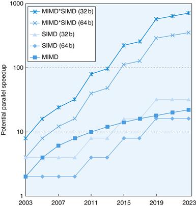
FIGURE 6.28 Potential speedup via parallelism from MIMD, SIMD, and both MIMD and SIMD over time for x86 computers.
This figure assumes that two cores per chip for MIMD will be added every two years and the number of operations for SIMD will double every four years.
■ The use of parallel processing in domains such as scientific and engineering computation is popular. This application domain has an almost limitless thirst for more computation. It also has many applications that have lots of natural concurrency. Once again, clusters dominate this application area. For example, using the 2012 Top 500 report, clusters are responsible for more than 80% of the 500 fastest Linpack results.
■ All desktop and server microprocessor manufacturers are building multiprocessors to achieve higher performance, so, unlike in the past, there is no easy path to higher performance for sequential applications. As we said earlier, sequential programs are now slow programs. Hence, programmers who need higher performance must parallelize their codes or write new parallel processing programs.
■ In the past, microprocessors and multiprocessors were subject to different definitions of success. When scaling uniprocessor performance, microprocessor architects were happy if single thread performance went up by the square root of the increased silicon area. Thus, they were happy with sublinear performance in terms of resources. Multiprocessor success used to be defined as linear speedup as a function of the number of processors, assuming that the cost of purchase or cost of administration of n processors was n times as much as one processor. Now that parallelism is happening on-chip via multicore, we can use the traditional microprocessor metric of being successful with sublinear performance improvement.
■ The success of just-in-time runtime compilation and autotuning makes it feasible to think of software adapting itself to take advantage of the increasing number of cores per chip, which provides flexibility that is not available when limited to static compilers.
■ Unlike in the past, the open source movement has become a critical portion of the software industry. This movement is a meritocracy, where better engineering solutions can win the mind share of the developers over legacy concerns. It also embraces innovation, inviting change to old software and welcoming new languages and software products. Such an open culture could be extremely helpful in this time of rapid change.
To motivate readers to embrace this revolution, we demonstrated the potential of parallelism concretely for matrix multiply on the Intel Core i7 (Sandy Bridge) in the Going Faster sections of Chapters 3 to 6:
■ Data-level parallelism in Chapter 3 improved performance by a factor of 3.85 by executing four 64-bit floating-point operations in parallel using the 256-bit operands of the AVX instructions, demonstrating the value of SIMD.
■ Instruction-level parallelism in Chapter 4 pushed performance up by another factor of 2.3 by unrolling loops 4 times to give the out-of-order execution hardware more instructions to schedule.
■ Cache optimizations in Chapter 5 improved performance of matrices that didn’t fit into the L1 data cache by another factor of 2.0 to 2.5 by using cache blocking to reduce cache misses.
■ Thread-level parallelism in this chapter improved performance of matrices that don’t fit into a single L1 data cache by another factor of 4 to 14 by utilizing all 16 cores of our multicore chips, demonstrating the value of MIMD. We did this by adding a single line using an OpenMP pragma.
Using the ideas in this book and tailoring the software to this computer added 24 lines of code to DGEMM. For the matrix sizes of 32 x32, 160 x160, 480 x480, and 960 x960, the overall performance speedup from these ideas realized in those two-dozen lines of code is factors of 8, 39, 129, and 212!
This parallel revolution in the hardware/software interface is perhaps the greatest challenge facing the field in the last 60 years. You can also think of it as the greatest opportunity, as our Going Faster sections demonstrate. This revolution will provide many new research and business prospects inside and outside the IT field, and the companies that dominate the multicore era may not be the same ones that dominated the uniprocessor era. After understanding the underlying hardware trends and learning to adapt software to them, perhaps you will be one of the innovators who will seize the opportunities that are certain to appear in the uncertain times ahead. We look forward to benefiting from your inventions!

Historical Perspective and Further Reading
This section online gives the rich and often disastrous history of multiprocessors over the last 50 years.
References
1. Regnier G, Makineni S, Illikkal R, et al. TCP onloading for data center servers. IEEE Computer. 2004;37(11):48–58.
2. B. F. Cooper, A. Silberstein, E. Tam, R. Ramakrishnan, R. Sears. Benchmarking cloud serving systems with YCSB, In: Proceedings of the 1st ACM Symposium on Cloud computing, June 10–11, 2010, Indianapolis, Indiana, USA, doi:10.1145/1807128.1807152.
6.16 Exercises
6.1 First, write down a list of your daily activities that you typically do on a weekday. For instance, you might get out of bed, take a shower, get dressed, eat breakfast, dry your hair, brush your teeth. Make sure to break down your list so you have a minimum of 10 activities.
6.1.1 [5] <§6.2> Now consider which of these activities is already exploiting some form of parallelism (e.g., brushing multiple teeth at the same time, versus one at a time, carrying one book at a time to school, versus loading them all into your backpack and then carry them “in parallel”). For each of your activities, discuss if they are already working in parallel, but if not, why they are not.
6.1.2 [5] <§6.2> Next, consider which of the activities could be carried out concurrently (e.g., eating breakfast and listening to the news). For each of your activities, describe which other activity could be paired with this activity.
6.1.3 [5] <§6.2> For 6.1.2, what could we change about current systems (e.g., showers, clothes, TVs, cars) so that we could perform more tasks in parallel?
6.1.4 [5] <§6.2> Estimate how much shorter time it would take to carry out these activities if you tried to carry out as many tasks in parallel as possible.
6.2 You are trying to bake 3 blueberry pound cakes. Cake ingredients are as follows:
1 cup butter, softened
1 cup sugar
4 large eggs
1 teaspoon vanilla extract
1/2 teaspoon salt
1/4 teaspoon nutmeg
1 1/2 cups flour
1 cup blueberries
The recipe for a single cake is as follows:
Step 1: Preheat oven to 325°F (160°C). Grease and flour your cake pan.
Step 2: In large bowl, beat together with a mixer butter and sugar at medium speed until light and fluffy. Add eggs, vanilla, salt and nutmeg. Beat until thoroughly blended. Reduce mixer speed to low and add flour, 1/2 cup at a time, beating just until blended.
Step 3: Gently fold in blueberries. Spread evenly in prepared baking pan. Bake for 60 minutes.
6.2.1 [5] <§6.2> Your job is to cook 3 cakes as efficiently as possible. Assuming that you only have one oven large enough to hold one cake, one large bowl, one cake pan, and one mixer, come up with a schedule to make three cakes as quickly as possible. Identify the bottlenecks in completing this task.
6.2.2 [5] <§6.2> Assume now that you have three bowls, 3 cake pans and 3 mixers. How much faster is the process now that you have additional resources?
6.2.3 [5] <§6.2> Assume now that you have two friends that will help you cook, and that you have a large oven that can accommodate all three cakes. How will this change the schedule you arrived at in Exercise 6.2.1 above?
6.2.4 [5] <§6.2> Compare the cake-making task to computing 3 iterations of a loop on a parallel computer. Identify data-level parallelism and task-level parallelism in the cake-making loop.
6.3 Many computer applications involve searching through a set of data and sorting the data. A number of efficient searching and sorting algorithms have been devised in order to reduce the runtime of these tedious tasks. In this problem we will consider how best to parallelize these tasks.
6.3.1 [10] <§6.2> Consider the following binary search algorithm (a classic divide and conquer algorithm) that searches for a value X in an sorted N-element array A and returns the index of matched entry:
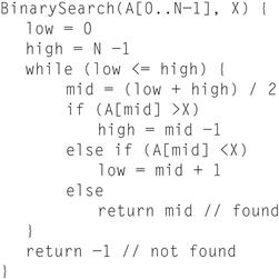
Assume that you have Y cores on a multicore processor to run BinarySearch. Assuming that Y is much smaller than N, express the speedup factor you might expect to obtain for values of Y and N. Plot these on a graph.
6.3.2 [5] <§6.2> Next, assume that Y is equal to N. How would this affect your conclusions in your previous answer? If you were tasked with obtaining the best speedup factor possible (i.e., strong scaling), explain how you might change this code to obtain it.
6.4 Consider the following piece of C code:
for (j=2;j<1000;j++)
D[j] = D[j−1]+D[j−2];
The MIPS code corresponding to the above fragment is:
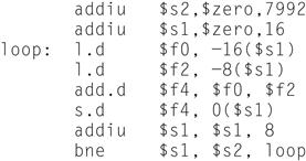
Instructions have the following associated latencies (in cycles):
![]()
6.4.1 [10] <§6.2> How many cycles does it take for all instructions in a single iteration of the above loop to execute?
6.4.2 [10] <§6.2> When an instruction in a later iteration of a loop depends upon a data value produced in an earlier iteration of the same loop, we say that there is a loop carried dependence between iterations of the loop. Identify the loop-carried dependences in the above code. Identify the dependent program variable and assembly-level registers. You can ignore the loop induction variable j.
6.4.3 [10] <§6.2> Loop unrolling was described in Chapter 4. Apply loop unrolling to this loop and then consider running this code on a 2-node distributed memory message passing system. Assume that we are going to use message passing as described in Section 6.7, where we introduce a new operation send (x, y) that sends to node x the value y, and an operation receive( ) that waits for the value being sent to it. Assume that send operations take a cycle to issue (i.e., later instructions on the same node can proceed on the next cycle), but take 10 cycles be received on the receiving node. Receive instructions stall execution on the node where they are executed until they receive a message. Produce a schedule for the two nodes assuming an unroll factor of 4 for the loop body (i.e., the loop body will appear 4 times). Compute the number of cycles it will take for the loop to run on the message passing system.
6.4.4 [10] <§6.2> The latency of the interconnect network plays a large role in the efficiency of message passing systems. How fast does the interconnect need to be in order to obtain any speedup from using the distributed system described in Exercise 6.4.3?
6.5 Consider the following recursive mergesort algorithm (another classic divide and conquer algorithm). Mergesort was first described by John Von Neumann in 1945. The basic idea is to divide an unsorted list x of m elements into two sublists of about half the size of the original list. Repeat this operation on each sublist, and continue until we have lists of size 1 in length. Then starting with sublists of length 1, “merge” the two sublists into a single sorted list.
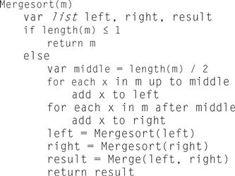
The merge step is carried out by the following code:
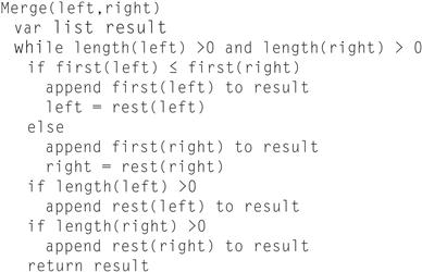
6.5.1 [10] <§6.2> Assume that you have Y cores on a multicore processor to run MergeSort. Assuming that Y is much smaller than length(m), express the speedup factor you might expect to obtain for values of Y and length(m). Plot these on a graph.
6.5.2 [10] <§6.2> Next, assume that Y is equal to length (m). How would this affect your conclusions your previous answer? If you were tasked with obtaining the best speedup factor possible (i.e., strong scaling), explain how you might change this code to obtain it.
6.6 Matrix multiplication plays an important role in a number of applications. Two matrices can only be multiplied if the number of columns of the first matrix is equal to the number of rows in the second.
Let’s assume we have an m×n matrix A and we want to multiply it by an n×p matrix B. We can express their product as an m×p matrix denoted by AB (or A·B). If we assign C=AB, and ci,j denotes the entry in Cat position (i, j), then for each element i and j with 1≤i≤m and 1≤j≤p. Now we want to see if we can parallelize the computation of C. Assume that matrices are laid out in memory sequentially as follows: a1,1, a2,1, a3,1, a4,1, …, etc.
6.6.1 [10] <§6.5> Assume that we are going to compute C on both a single core shared memory machine and a 4-core shared-memory machine. Compute the speedup we would expect to obtain on the 4-core machine, ignoring any memory issues.
6.6.2 [10] <§6.5> Repeat Exercise 6.6.1, assuming that updates to C incur a cache miss due to false sharing when consecutive elements are in a row (i.e., index i) are updated.
6.6.3 [10] <§6.5> How would you fix the false sharing issue that can occur?
6.7 Consider the following portions of two different programs running at the same time on four processors in a symmetric multicore processor (SMP). Assume that before this code is run, both x and y are 0.
Core 1: x = 2;
Core 2: y = 2;
Core 3: w = x + y + 1;
Core 4: z = x + y;
6.7.1 [10] <§6.5> What are all the possible resulting values of w, x, y, and z? For each possible outcome, explain how we might arrive at those values. You will need to examine all possible interleavings of instructions.
6.7.2 [5] <§6.5> How could you make the execution more deterministic so that only one set of values is possible?
6.8 The dining philosopher’s problem is a classic problem of synchronization and concurrency. The general problem is stated as philosophers sitting at a round table doing one of two things: eating or thinking. When they are eating, they are not thinking, and when they are thinking, they are not eating. There is a bowl of pasta in the center. A fork is placed in between each philosopher. The result is that each philosopher has one fork to her left and one fork to her right. Given the nature of eating pasta, the philosopher needs two forks to eat, and can only use the forks on her immediate left and right. The philosophers do not speak to one another.
6.8.1 [10] <§6.7> Describe the scenario where none of philosophers ever eats (i.e., starvation). What is the sequence of events that happen that lead up to this problem?
6.8.2 [10] <§6.7> Describe how we can solve this problem by introducing the concept of a priority? But can we guarantee that we will treat all the philosophers fairly? Explain.
Now assume we hire a waiter who is in charge of assigning forks to philosophers. Nobody can pick up a fork until the waiter says they can. The waiter has global knowledge of all forks. Further, if we impose the policy that philosophers will always request to pick up their left fork before requesting to pick up their right fork, then we can guarantee to avoid deadlock.
6.8.3 [10] <§6.7> We can implement requests to the waiter as either a queue of requests or as a periodic retry of a request. With a queue, requests are handled in the order they are received. The problem with using the queue is that we may not always be able to service the philosopher whose request is at the head of the queue (due to the unavailability of resources). Describe a scenario with 5 philosophers where a queue is provided, but service is not granted even though there are forks available for another philosopher (whose request is deeper in the queue) to eat.
6.8.4 [10] <§6.7> If we implement requests to the waiter by periodically repeating our request until the resources become available, will this solve the problem described in Exercise 6.8.3? Explain.
6.9 Consider the following three CPU organizations:
CPU SS: A 2-core superscalar microprocessor that provides out-of-order issue capabilities on 2 function units (FUs). Only a single thread can run on each core at a time.
CPU MT: A fine-grained multithreaded processor that allows instructions from 2 threads to be run concurrently (i.e., there are two functional units), though only instructions from a single thread can be issued on any cycle.
CPU SMT: An SMT processor that allows instructions from 2 threads to be run concurrently (i.e., there are two functional units), and instructions from either or both threads can be issued to run on any cycle.
Assume we have two threads X and Y to run on these CPUs that include the following operations:
|
Thread X |
Thread Y |
|
A1 – takes 3 cycles to execute |
B1 – take 2 cycles to execute |
|
A2 – no dependences |
B2 – conflicts for a functional unit with B1 |
|
A3 – conflicts for a functional unit with A1 |
B3 – depends on the result of B2 |
|
A4 – depends on the result of A3 |
B4 – no dependences and takes 2 cycles to execute |
Assume all instructions take a single cycle to execute unless noted otherwise or they encounter a hazard.
6.9.1 [10] <§6.4> Assume that you have 1 SS CPU. How many cycles will it take to execute these two threads? How many issue slots are wasted due to hazards?
6.9.2 [10] <§6.4> Now assume you have 2 SS CPUs. How many cycles will it take to execute these two threads? How many issue slots are wasted due to hazards?
6.9.3 [10] <§6.4> Assume that you have 1 MT CPU. How many cycles will it take to execute these two threads? How many issue slots are wasted due to hazards?
6.10 Virtualization software is being aggressively deployed to reduce the costs of managing today’s high performance servers. Companies like VMWare, Microsoft and IBM have all developed a range of virtualization products. The general concept, described in Chapter 5, is that a hypervisor layer can be introduced between the hardware and the operating system to allow multiple operating systems to share the same physical hardware. The hypervisor layer is then responsible for allocating CPU and memory resources, as well as handling services typically handled by the operating system (e.g., I/O).
Virtualization provides an abstract view of the underlying hardware to the hosted operating system and application software. This will require us to rethink how multicore and multiprocessor systems will be designed in the future to support the sharing of CPUs and memories by a number of operating systems concurrently.
6.10.1 [30] <§6.4> Select two hypervisors on the market today, and compare and contrast how they virtualize and manage the underlying hardware (CPUs and memory).
6.10.2 [15] <§6.4> Discuss what changes may be necessary in future multicore CPU platforms in order to better match the resource demands placed on these systems. For instance, can multithreading play an effective role in alleviating the competition for computing resources?
6.11 We would like to execute the loop below as efficiently as possible. We have two different machines, a MIMD machine and a SIMD machine.
for (i=0; i < 2000; i++)
for (j=0; j<3000; j++)
X_array[i][j] = Y_array[j][i] + 200;
6.11.1 [10] <§6.3> For a 4 CPU MIMD machine, show the sequence of MIPS instructions that you would execute on each CPU. What is the speedup for this MIMD machine?
6.11.2 [20] <§6.3> For an 8-wide SIMD machine (i.e., 8 parallel SIMD functional units), write an assembly program in using your own SIMD extensions to MIPS to execute the loop. Compare the number of instructions executed on the SIMD machine to the MIMD machine.
6.12 A systolic array is an example of an MISD machine. A systolic array is a pipeline network or “wavefront” of data processing elements. Each of these elements does not need a program counter since execution is triggered by the arrival of data. Clocked systolic arrays compute in “lock-step” with each processor undertaking alternate compute and communication phases.
6.12.1 [10] <§6.3> Consider proposed implementations of a systolic array (you can find these in on the Internet or in technical publications). Then attempt to program the loop provided in Exercise 6.11 using this MISD model. Discuss any difficulties you encounter.
6.12.2 [10] <§6.3> Discuss the similarities and differences between an MISD and SIMD machine. Answer this question in terms of data-level parallelism.
6.13 Assume we want to execute the DAXP loop show on page 511 in MIPS assembly on the NVIDIA 8800 GTX GPU described in this chapter. In this problem, we will assume that all math operations are performed on single-precision floating-point numbers (we will rename the loop SAXPY). Assume that instructions take the following number of cycles to execute.
![]()
6.13.1 [20] <§6.6> Describe how you will constructs warps for the SAXP loop to exploit the 8 cores provided in a single multiprocessor.
6.14 Download the CUDA Toolkit and SDK from http://www.nvidia.com/object/cuda_get.html. Make sure to use the “emurelease” (Emulation Mode) version of the code (you will not need actual NVIDIA hardware for this assignment). Build the example programs provided in the SDK, and confirm that they run on the emulator.
6.14.1 [90] <§6.6> Using the “template” SDK sample as a starting point, write a CUDA program to perform the following vector operations:
1) a−b (vector-vector subtraction)
2) a·b (vector dot product)
The dot product of two vectors a=[a1, a2, … , an] and b=[b1, b2, … , bn] is defined as:
![]()
Submit code for each program that demonstrates each operation and verifies the correctness of the results.
6.14.2 [90] <§6.6> If you have GPU hardware available, complete a performance analysis your program, examining the computation time for the GPU and a CPU version of your program for a range of vector sizes. Explain any results you see.
6.15 AMD has recently announced that they will be integrating a graphics processing unit with their×86 cores in a single package, though with different clocks for each of the cores. This is an example of a heterogeneous multiprocessor system which we expect to see produced commericially in the near future. One of the key design points will be to allow for fast data communication between the CPU and the GPU. Presently communications must be performed between discrete CPU and GPU chips. But this is changing in AMDs Fusion architecture. Presently the plan is to use multiple (at least 16) PCI express channels for facilitate intercommunication. Intel is also jumping into this arena with their Larrabee chip. Intel is considering to use their QuickPath interconnect technology.
6.15.1 [25] <§6.6> Compare the bandwidth and latency associated with these two interconnect technologies.
6.16 Refer to Figure 6.14b, which shows an n-cube interconnect topology of order 3 that interconnects 8 nodes. One attractive feature of an n-cube interconnection network topology is its ability to sustain broken links and still provide connectivity.
6.16.1 [10] <§6.8> Develop an equation that computes how many links in the n-cube (where n is the order of the cube) can fail and we can still guarantee an unbroken link will exist to connect any node in the n-cube.
6.16.2 [10] <§6.8> Compare the resiliency to failure of n-cube to a fully-connected interconnection network. Plot a comparison of reliability as a function of the added number of links for the two topologies.
6.17 Benchmarking is field of study that involves identifying representative workloads to run on specific computing platforms in order to be able to objectively compare performance of one system to another. In this exercise we will compare two classes of benchmarks: the Whetstone CPU benchmark and the PARSEC Benchmark suite. Select one program from PARSEC. All programs should be freely available on the Internet. Consider running multiple copies of Whetstone versus running the PARSEC Benchmark on any of systems described in Section 6.11.
6.17.1 [60] <§6.10> What is inherently different between these two classes of workload when run on these multicore systems?
6.17.2 [60] <§6.10> In terms of the Roofline Model, how dependent will the results you obtain when running these benchmarks be on the amount of sharing and synchronization present in the workload used?
6.18 When performing computations on sparse matrices, latency in the memory hierarchy becomes much more of a factor. Sparse matrices lack the spatial locality in the data stream typically found in matrix operations. As a result, new matrix representations have been proposed.
One the earliest sparse matrix representations is the Yale Sparse Matrix Format. It stores an initial sparse m×n matrix, M in row form using three one-dimensional arrays. Let R be the number of nonzero entries in M. We construct an array A of length R that contains all nonzero entries of M (in left-to-right top-to-bottom order). We also construct a second array IA of length m+1 (i.e., one entry per row, plus one). IA(i) contains the index in A of the first nonzero element of row i. Row i of the original matrix extends from A(IA(i)) to A(IA(i+1)−1). The third array, JA, contains the column index of each element of A, so it also is of length R.
6.18.1 [15] <§6.10> Consider the sparse matrix X below and write C code that would store this code in Yale Sparse Matrix Format.
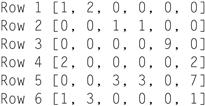
6.18.2 [10] <§6.10> In terms of storage space, assuming that each element in matrix X is single precision floating point, compute the amount of storage used to store the Matrix above in Yale Sparse Matrix Format.
6.18.3 [15] <§6.10> Perform matrix multiplication of Matrix X by Matrix Y shown below.
[2, 4, 1, 99, 7, 2]
Put this computation in a loop, and time its execution. Make sure to increase the number of times this loop is executed to get good resolution in your timing measurement. Compare the runtime of using a naïve representation of the matrix, and the Yale Sparse Matrix Format.
6.18.4 [15] <§6.10> Can you find a more efficient sparse matrix representation (in terms of space and computational overhead)?
6.19 In future systems, we expect to see heterogeneous computing platforms constructed out of heterogeneous CPUs. We have begun to see some appear in the embedded processing market in systems that contain both floating point DSPs and a microcontroller CPUs in a multichip module package.
Assume that you have three classes of CPU:
CPU A—A moderate speed multicore CPU (with a floating point unit) that can execute multiple instructions per cycle.
CPU B—A fast single-core integer CPU (i.e., no floating point unit) that can execute a single instruction per cycle.
CPU C—A slow vector CPU (with floating point capability) that can execute multiple copies of the same instruction per cycle.
Assume that our processors run at the following frequencies:
|
CPU A |
CPU B |
CPU C |
|
1 GHz |
3 GHz |
250 MHz |
CPU A can execute 2 instructions per cycle, CPU B can execute 1 instruction per cycle, and CPU C can execute 8 instructions (though the same instruction) per cycle. Assume all operations can complete execution in a single cycle of latency without any hazards.
All three CPUs have the ability to perform integer arithmetic, though CPU B cannot perform floating point arithmetic. CPU A and B have an instruction set similar to a MIPS processor. CPU C can only perform floating point add and subtract operations, as well as memory loads and stores. Assume all CPUs have access to shared memory and that synchronization has zero cost.
The task at hand is to compare two matrices X and Y that each contain 1024×1024 floating point elements. The output should be a count of the number indices where the value in X was larger or equal to the value in Y.
6.19.1 [10] <§6.11> Describe how you would partition the problem on the 3 different CPUs to obtain the best performance.
6.19.2 [10] <§6.11> What kind of instruction would you add to the vector CPU C to obtain better performance?
6.20 Assume a quad-core computer system can process database queries at a steady state rate of requests per second. Also assume that each transaction takes, on average, a fixed amount of time to process. The following table shows pairs of transaction latency and processing rate.
|
Average Transaction Latency |
Maximum transaction processing rate |
|
1 ms |
5000/sec |
|
2 ms |
5000/sec |
|
1 ms |
10,000/sec |
|
2 ms |
10,000/sec |
For each of the pairs in the table, answer the following questions:
6.20.1 [10] <§6.11> On average, how many requests are being processed at any given instant?
6.20.2 [10] <§6.11> If move to an 8-core system, ideally, what will happen to the system throughput (i.e., how many queries/second will the computer process)?
6.20.3 [10] <§6.11> Discuss why we rarely obtain this kind of speedup by simply increasing the number of cores.
All materials on the site are licensed Creative Commons Attribution-Sharealike 3.0 Unported CC BY-SA 3.0 & GNU Free Documentation License (GFDL)
If you are the copyright holder of any material contained on our site and intend to remove it, please contact our site administrator for approval.
© 2016-2026 All site design rights belong to S.Y.A.