Knowledge-based Configuration: From Research to Business Cases, FIRST EDITION (2014)

Part II. Basics

Chapter 6. Configuration Knowledge Representation and Reasoning

Lothar Hotz^a, Alexander Felfernig^b, Markus Stumptner^c, Anna Ryabokon^d, Claire Bagley^e and Katharina Wolter^a, ^aHITeC e.V., University of Hamburg, Hamburg, Germany, ^bGraz University of Technology, Graz, Austria, ^cUniversity of South Australia, Adelaide, SA, Australia, ^dAlpen-Adria Universität Klagenfurt, Klagenfurt, Austria, ^eOracle Corporation, Burlington, MA, USA

Abstract

Configuration models specify the set of possible configurations (solutions). A configuration model together with a defined set of (customer) requirements are the major elements of a configuration task (problem). In this chapter, we discuss different knowledge representations that can be used for the definition of a configuration model. We provide examples that help to further develop the understanding of the underlying concepts and include a UML-based personal computer (PC) configuration model that is used as a reference example throughout this book.

Keywords

Knowledge-based Configuration; Knowledge Representation; Constraints; Feature Models; Unified Modelling Language; Description Logics; Answer Set Programming

Acknowledgments

The work presented in this chapter was partially funded by the Austrian research promotion agency (grant numbers: 827587 and 825071).

6.1 Introduction

There is quite a long history of research dedicated to the development of configuration knowledge representation languages (Felfernig et al., 2003; Günter and Kühn, 1999; Jüngst and Heinrich, 1998; Junker, 2006; Mailharro, 1998; McDermott, 1982; McGuinness and Wright, 1998; Mittal and Falkenhainer, 1990; Mittal and Frayman, 1989; Soininen et al., 1998). One of the first configuration systems was R1/XCON, which was built upon a rule-based representation language (McDermott, 1982; Soloway et al., 1987). Rule-based systems operate on a working memory that stores assertions made by rules. Rules are represented in an if-then style. If a rule is activated (given that the if condition is fulfilled) it can modify the contents of the working memory. Experiences showed that a major problem with rule-based systems is the intermingling of (product) domain knowledge and problem solving knowledge (see also Friedrich et al., 2014¹). A consequence is that if product knowledge is changed, rules related to the sequence in which components are integrated in a configuration have to be adapted as well, which triggers enormous maintenance overheads.² The shortcomings of rule-based approaches were the motivation for the development of model-based knowledge representations that support a clear separation of domain and problem solving knowledge. Mittal and Frayman (1989) introduced a model-based definition of a configuration task that is characterized by: (1) a description of generic components in terms of their properties and relationships and (2) user requirements and preferences regarding functional properties of the solution (configuration). This characterization is a major foundation for configuration research and industry (Junker, 2006). It also includes the idea of separating functional requirements (customer requirements) from the technical properties of a configurable product.

A major representative of model-based approaches are constraint-based systems (see, e.g., Freuder, 1997; Tsang, 1993). Related knowledge representations range from static constraint satisfaction (variables and constraints are predefined and are part of the search process from the very beginning (see, for example, Tsang, 1993), dynamic constraint satisfaction (variables are not necessarily active from the very beginning but can be activated within the scope of the search process; Mittal and Falkenhainer, 1990), to generative constraint satisfaction where components and related constraints are generated on-demand within the scope of the search process (see Stumptner et al., 1998). Generative approaches can also be denoted as component-oriented since component types (instead of variables) and meta (generic) constraints (instead of constraints) are taken into account as first-class entities. Examples of configuration knowledge representation in terms of a constraint satisfaction problem (CSP) will be provided in Section 6.2.

In the following, graphical representations have been developed with the goal of improving the accessibility (in terms of, e.g., understandability and maintainability) of configuration knowledge, which is crucial especially in commercial settings. One approach to the graphical representation of configuration models are feature models (see, e.g., Kang et al., 1990). Feature models can be represented in the form of a static constraint satisfaction problem (CSP; Tsang, 1993) or in the form of a SAT problem (Gomes et al., 2008).Neumann (1988) and Soininen et al. (1998) introduced configuration ontologies, which define relevant modeling concepts for configuration knowledge representation. These ontologies include modeling concepts that are typically provided in today’s commercial configuration environments; for example, component types, ports, and constraints. Similar ontological concepts as introduced, for example, by Neumann (1988) and Soininen et al. (1998) in terms of a UML profile for configuration knowledge representation, and a formalization of these concepts in first-order logic as well as in description logic has been proposed by Felfernig (2007), and Felfernig et al. (2000a, 2003). Note that in this chapter we focus on the representation of product-related configuration knowledge; knowledge representations related to incremental configuration processes (Sabin and Weigel, 1998) are discussed in detail in Leitner et al. (2014),³ Hotz and Wolter (2014),⁴ and Hotz and Günter (2014).⁵

With this chapter, we provide an overview of modeling concepts that are relevant for configuration knowledge representation. In Subsection 6.2.1, we introduce static constraint satisfaction problems as a basic representation mechanism for configuration knowledge. In Subsection 6.2.2, we introduce two types of advanced CSP representations that are dynamic and generative constraint satisfaction problems. Thereafter, in Section 6.3, we discuss graphical configuration knowledge representations (feature models and UML models). On the basis of the latter we introduce a personal computer configuration model. In the other chapters of this book, this UML model is adapted and extended where needed. In Section 6.4, we give an overview of different logic-based approaches to configuration knowledge representation. This chapter concludes with a discussion of major advantages and disadvantages of different types of configuration knowledge representations.

6.2 Constraint-Based Knowledge Representation

6.2.1 Static Constraint Satisfaction

“Constraint technologies are one of the closest approaches computer science has yet made to the Holy Grail of programming: a user states the problem, the computer solves it.” (Freuder, 1997). Constraint technologies are one of the most successfully applied technologies of Artificial Intelligence (AI) in commercial settings (Brailsford et al., 1999). With these technologies, the knowledge acquisitionbottleneck⁶ is tackled by the means of an easy to understand and easy to use technology. Application examples are configuration (Fleischanderl et al., 1998; Mittal and Frayman, 1989), scheduling (Pinedo, 2012), and recommender systems (Felfernig and Burke, 2008; Jannach et al., 2010). Constraint-based representationsare widely used for the definition of configuration models (see, Junker and Mailharro, 2003;Mailharro, 1998). We first focus on static constraint satisfaction problems (SCSPs).

Constraint Satisfaction Problem and Solution

We will now introduce a definition of a constraint satisfaction problem (CSP) and its solution. This definition will then be used as a basis for defining a configuration task (problem) and a corresponding configuration (solution).

Definition

Constraint Satisfaction Problem – CSP

A constraint satisfaction problem (CSP) can be defined by a triple (V, D, C) where V is a set of finite domain variables , D represents variable domains , and C represents a set of constraints defining restrictions on the possible combinations of variable values ().

A solution for a given CSP = (V, D, C) can be defined as follows.

Definition

CSP Solution

A solution for a given CSP = (V, D, C) is represented by an assignment where . is required to be complete; that is each variable of the CSP definition has a value in and is consistent (i.e., fulfills the constraints in ).

Configuration Task and Solution

Based on this definition of a CSP, we can now introduce the definition of a configuration task (problem) and a corresponding configuration (solution). We introduce two sets of constraints that describe (1) the configuration knowledge base () and (2) the user requirements ().

Definition

Configuration Task

A configuration task can be defined as a CSP (V, D, C) where , and . represents the configuration knowledge base (the configuration model) and represents a set of user (customer) requirements.

Definition

Configuration

A configuration (solution) S for a given configuration task (V, D, ) is represented by an assignment where and S is complete and consistent with the constraints in .

This definition of a configuration task and its solution is exploited by some of the chapters in this book. This approach to represent a configuration task is primarily used in situations where all variables of the problem definition are relevant for the solution. To better understand the pragmatics of these definitions, we will now present two example configuration models: a configuration model for map coloring and a mobile phone configuration model.

Example: Map Configuration (Map Coloring)

Map-coloring can be interpreted as a simple configuration task (problem). The goal of this configuration task is to assign a color to each of the regions of a map in such a way that for each region on the map the following property holds: all regions that are direct neighbors of must have a different color (different from the color of ).

As an example, we take the map of Australia (see also Russel and Norvig, 2003), which includes the regions of Western Australia (WA), Northern Territory (NT), South Australia (SA), Queensland (Q), New South Wales (NSW), Victoria (V), and Tasmania (T) (see Figure 6.1). These regions must be colored with the colors red, green, and black.

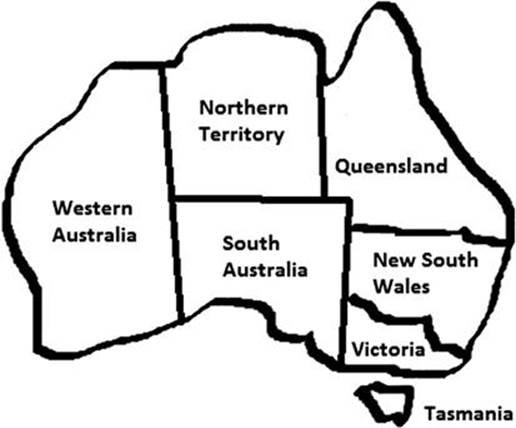
FIGURE 6.1 Territory map of Australia.

Based on this characterization of a map coloring configuration problem, we can define the corresponding configuration task .

= {WA, NT, SA, Q, NSW, V, T}

= {dom(WA)={r,g,b}, dom(NT)={r,g,b}, dom(SA)={r,g,b}, dom(Q)= {r,g,b}, dom(NSW)={r,g,b}, dom(V)={r,g,b}, dom(T)={r,g,b}}

Finally, we introduce the set of constraints to be taken into account when configuring (coloring) a map. The elements of are those constraints that are defining the restrictions regarding the color combinations of neighborhood territories.

= {}

A CSP can also be represented graphically in terms of nodes (the variables) and the corresponding constraints (arcs between the variables); Figure 6.2 shows a graphical depiction of the map coloring configuration model.

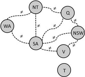
FIGURE 6.2 Map coloring configuration model: graphical representation of a CSP where the nodes represent the variables and the arcs represent constraints.

Customer requirementsin this context can be preferences (in terms of initial settings) regarding the coloring of the map. For example, we could introduce the singleton requirement ; that is, the color of Western Australia (WA) should be red (). Then is consistent; that is, we are able to determine a solution for the map coloring (configuration) problem.

Example: Mobile Phone Configuration

The following configuration model of a mobile phone is based on the model of a mobile phone software product lines (adapted from Benavides et al., 2010). We will provide a formalization of this model on the basis of the definition of a configuration task given in Subsection 6.2.1.⁷ See Figure 6.3 for a graphical depiction of the mobile phone configuration model.

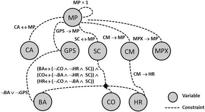
FIGURE 6.3 Simple Mobile Phone configuration model (represented as CSP). An abbreviation is used for the constraint representation; for example, CA MP is the short form of . Mobile Phone, Calls, GPS, Screen, Camera, MPX Player, Basic, Color, High Resolution.

Our Mobile Phone (MP) model consists of the following elements: each mobile phone has two mandatory elements that are the support of Calls (CA) and the availability of a Screen (SC). A Screen can either be of type Basic (BA), Color (CO), or HighResolution (HR). A mobile phone can (but does not have to) be equipped with a GPS (GPS) feature. Furthermore, a mobile phone can include additional media equipment (Camera (CM) and MPX Player (MPX)). When equipped with a GPS, then the phone’s Screen can’t be of type Basic. A phone with a Camera must be equipped with a HighResolution Screen.

Based on this characterization of the basic properties of our example mobile phone, we can introduce the following configuration task ().

{MP, CA, GPS, BA, CO, HR, SC, CM, MPX}

Since we are interested in defining the possible combinations of mobile phone features, we assign to each of the feature variables in the domain {1,0} ({true, false} is possible as well). The semantics of 1 (resp. 0) is that a feature is active (resp. inactive); that is, included or not included in a configuration.

D {dom(MP) {1, 0}, dom(CA) {1, 0}, dom(GPS) {1, 0}, dom(BA) {1, 0}, dom(CO) {1, 0}, dom(HR) {1, 0}, dom(SC) {1, 0}, dom(CM) {1, 0}, dom(MPX) {1, 0}}

Finally, we specify the constraints .⁸ Since we are not interested in empty configurations, we introduce the constraint MP 1.

{MP 1, CA MP, GPS MP, SC MP, CM MP, MPX MP, (BA ( CO HR SC)) (CO ( BA HR SC)) (HR ( CO BA SC)), BA GPS, CM HR}

Customer requirementsregarding a concrete mobile phone configuration could be the following: ; that is, GPS should be included. In our example, is consistent and a possible configuration (solution) is:

Solution Search in Static CSPs

There is plenty of literature on algorithms that can be used for solving static constraint satisfaction problems (e.g., Mackworth, 1977; Rossi et al., 2006; Russel and Norvig, 2003; Tsang, 1993). The basic approach of CSP algorithms is to apply backtracking in combination with a couple of additional mechanisms that altogether focus on variable domain size reduction during search (Russel and Norvig, 2003). One basic principle for reducing the domain size of variables is node-consistency, which requires that those values of a variable domain that are inconsistent with an unary constraintare eliminated as options (for these options there does not exist a solution). Arc-consistency (AC)is a property that must be fulfilled by combinations of variables and that are connected via abinary constraint ⁹: each value in the domain of must have at least one corresponding value in the domain of such that is fulfilled. Note that arc-consistency is directed; if variable is arc-consistent with variable this does not necessarily mean that is arc-consistent with . In the following example we take a look at the variables WA and NT of our map configuration (coloring) example (see Figure 6.2). Although AC is restricted to binary constraints, this does not restrict its applicability since every n-ary constraint can be transformed into a corresponding set of binary constraints (e.g., Bacchus and vanBeek, 1998).

Example of node-consistency and arc-consistency. The original domain of = {r,g,b}. Since we defined as a requirement, is node-consistent and the values {g,b} get removed from its domain. In order to ensure arc-consistency between and , the value {r} needs to be removed from ’s domain definition. Now, each value in the new domain of has a consistent corresponding value in the domain of and vice versa.

Another important principle in variable domain size reduction is forward checking: Depending on the value selected for the current variable, the values of the instantiated variables that can’t be a support for the selected value are eliminated from their corresponding domains. An example is depicted in Figure 6.4.

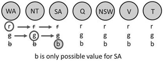
FIGURE 6.4 A simple example of forward checking. The variables and already have assigned values ( and ). The only possible remaining value for is ; and do not have to be checked for consistency with the settings of and .

Search algorithms for CSPs are able to support optimization,which helps to minimize (e.g., the overall price of a configuration) or maximize (e.g., the failure safety of an equipment) solution parameters (Pitiot et al., 2013).

Finally, tuning the performance of solution search is typically done with basic strategies of variable and value orderings (Russel and Norvig, 2003), with advanced approaches such as symmetry breaking (Kiziltan and Hnich, 2001) and machine learning based acquisition of search strategies (Terashima-Marin et al., 2008), with local search algorithms (Li et al., 2006), and different techniques of knowledge compilation such as binary decision diagrams (BDDs;Andersen et al., 2010) and solution automata (Amilhastre et al., 2002). For further literature on related algorithms and optimization approaches we refer to Brailsford et al. (1999); Rossi et al. (2006); Russel and Norvig (2003), and Tsang (1993).

Excursus: SAT Problems

For a given propositional formula, the goal of SAT solving (see, e.g., Claessen et al., 2008) is the determination of a variable assignment such that the formula evaluates to true. A propositional logic formula is in a conjunctive normal form (CNF) when it is represented in the form of conjunctions of disjunctions of literals. For a Boolean variable , a literal is defined as or its negation . Each of the disjunctions is denoted as a clause. A SAT problem (satisfiability problem) is to identify an assignment to the given Boolean variables in such a way that the mentioned formula in CNF evaluates to true. This is the case if each clause has at least one literal that evaluates to true. For a more detailed discussion of SAT solving and related algorithms, refer to Claessen et al. (2008). An example of the translation of a given static CSP into a corresponding SAT representation follows.

Example: SAT encoding of a static CSP. In order to show the basic principle of how to translate a static CSP into a corresponding SAT representation, we take the variables and from our working example (map coloring). In a static CSP representation the variable domains can be specified as dom()= {r,g,b} and dom()= {r,g,b}. In the corresponding SAT representation we have to introduce Boolean variables where each domain value of the original variables is represented by its own (Boolean) variable. In our example this translation results in the variables . Each of these variables has the domain {true, false} ({1,0}). The translation of the constraint into a clausal form could look like: . With this, we assure that (1) the two territories do not have the same color and (2) both territories have a color assigned.

As can easily be seen, our Mobile Phone configuration model can directly be translated into a corresponding SAT representation, since the variable domains in the CSP are already of type Boolean. For further related work refer to Janota (2008) and Janota et al. (2010).

6.2.2 Advanced CSP Approaches

On the basis of the static CSP approach, numerous extensions have been implemented in order to improve expressiveness and the efficiency of the underlying reasoning algorithms. An in-depth analysis of existing CSP variants is beyond the scope of this book; however, we will now discuss some representative ones that have found their way into commercial configuration environments.

Dynamic Constraint Satisfaction

Configuration tasks very often include variables that do not have to be taken into account in specific configuration contexts. For instance, in our mobile phone configuration example, the variable Camera is not relevant if the user is interested only in monochrome (basic) displays. In the mobile phone configuration example in Subsection 6.2.1, the property of variable irrelevance is implemented in terms of feature deactivation; that is, if no Camera is part of the configuration, the value of this variable is set to (false). However, if we want to introduce a variable Camera with the domain {TypeA, TypeB, TypeC} representing three different camera types, we would have to introduce an additional domain value noval that expresses the fact that the camera is not part of the configuration. As can be seen from this simple example, there is a need to include concepts that support reasoning over variable states (active, inactive). In order to take into account the requirement of leaving out irrelevant variables during the search process, Mittal and Falkenhainer (1990) introduced the concept of dynamic constraint satisfaction (DCSP), where a constraint solver is also able to reason about the activity states of variables. The following example shows such an activation constraint.

Example of an activation constraint. For a variable CM (the camera) with the domain {TypeA, TypeB, TypeC} we could define the following activation constraint: HighResolution (HR) = yes active(CM). If the precondition is not fulfilled, there is no need for CM to get assigned a value (i.e., be activated).

Such a reasoning about activity states in DCSPs is based on predefined activity constraints. A formal discussion of the properties of DCSPs can be found in Bowen and Bahler (1991). The concept of variable activation has also been applied in other approaches. For example, generative constraint satisfaction (GCSP) based systems (Stumptner et al., 1998) generalize the concept of variable activation to the concept of component and constraint activation. The configuration environment of SIEMENS is based on such a generative approach (see also Falkner and Schreiner, 2014).¹⁰

Generative Constraint Satisfaction

Major drawbacks of static (and dynamic) CSPs include representational limits in terms of dealing with variables and variable values instead of component types and corresponding components (instances). Another disadvantage is that static CSPs are limited with regard to the description of configuration problems in which the size and structure of configurations cannot be estimated beforehand. Generative constraint satisfaction (GCSP) helps to overcome these problems by moving variables and corresponding constraints to the level of component types and meta-constraints (generic constraints). Generic constraints (constraint schemata) help to identify and generate relevant additional components and variables that are relevant in the current configuration context.

Constraints are referred to as “generic” since they apply individually to all components of the types on which the constraints are defined. For example, a constraint preventing a particular type of CPU from being placed on a particular type of Motherboard applies to all CPUs of that type although it is only defined in the knowledge base once. Components in GCSP settings are represented in terms of a finite domain variable (the domain of the variable corresponds to the different types a component can take). Activation constraints are used, for example, to generate new property variables based on the assignment of a type to a component variable. A Generative Constraint Satisfaction Problem (GCSP) can be defined as follows (Stumptner et al., 1998).

Definition (Generative Constraint Satisfaction Problem – GCSP). A generative constraint satisfaction problem can be defined by a triple (CV, P, ) where is a possibly infinite set of component variables. The domain of each variable from CV is a finite set = {} of component types. is a set of property (attribute) names. Furthermore, there exists a set } of domains and a function that maps pairs of the form (property name, type) to elements of . The sets are called atomic domains (i.e., they contain numeric or symbolic values, but are distinct from ). The name of a property variable is composed from the name of the originating component and the property name; for example, if property is defined for component , then the property variable is named . Finally, is a finite set of generic constraints including activation and resource constraints.

GCSP representations allow the definition of ports that represent connection points between different components. In GCSPs (Stumptner et al., 1998), ports are represented by properties (attributes) that permit other components as values. Partonomies (part-of structures; see Subsection 6.3.2) can be represented on the basis of such port definitions. Inheritance relationships (related to a generation hierarchy) are represented on the basis of (generic) constraints that refer to component type domains.

Example GCSP component type. A component type PC (P) can be represented as follows using a GCSP-style notation (see, e.g. Stumptner et al., 1998). This definition of the basic properties of a PC is related to the graphical configuration model depicted in Figure 6.7. As can easily be seen, GCSP approaches have a more intuitive knowledge representation, which is inspired by object-oriented data models combined with constraints (see, e.g., Bowen and Bahler, 1991; Neumann 1988; Puget and Albert, 1991).

PC P DESCRIPTION:

P.name := [String];

P.price := [Integer];

P.usage := {‘internet’,‘scientific’,‘multimedia’};

P.efficiency := {‘A’,‘B’,‘C’};

P.PORTS := {screen-of-pc-1[Screen], screen-of-pc-2[Screen],

hdunit-of-pc-1[HDUnit], …};

P.screens := <screen-of-pc-1,screen-of-pc-2>;

P.mb := <mb-of-pc-1>;

P.hdunits := <hdunit-of-pc-1,hdunit-of-pc-2>;

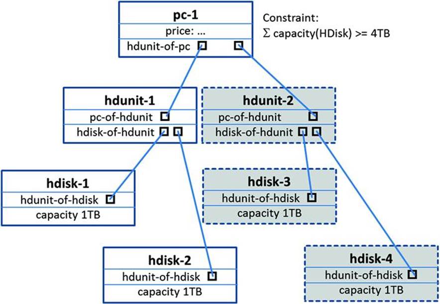
FIGURE 6.5 Simple GCSP dynamic component creation example. The constraint representation is simplified (i.e., it does not directly correspond to the GCSP constraint representation used in Stumptner et al., 1998).

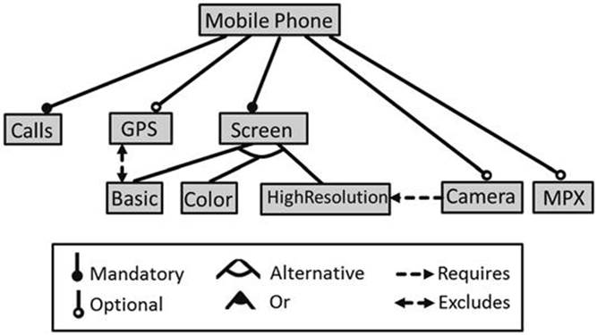
FIGURE 6.6 Feature model of a mobile phone (adapted version of Benavides et al., 2010). This feature model is equivalent to the constraint-based representation of Figure 6.3.

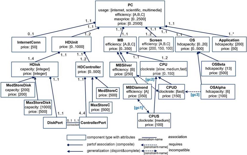
FIGURE 6.7 PC configuration model in UML. In addition to the included constraints {}, {} are introduced in Table 6.2.

GCSP constraints are represented in the context of a specific component type. As such this approach is very similar to constraint-including object-oriented languages such as the Unified Modeling Language (Booch et al., 2005) that includes the Object Constraint Language (OCL; Warmer and Kleppe, 2003). For an overview of the application of UML and OCL for configuration knowledge representation refer to Felfernig (2007) and Felfernig et al. (2000a). An example of a UML-based configuration model is introduced in Subsection 6.3.2.

Example GCSP constraint. A GCSP constraint that describes the fact that the energy efficiency required by the user must be supported by the motherboard mb, can be represented as follows. This example shows how constraints can “navigate” through the component partonomy defined for the GCSP.

PC P DESCRIPTION:

P.efficiency = P.mb.efficiency;

Usually, GCSP environments include a graphical front end that helps to define the configuration model more easily in an object-oriented fashion. Such an abstraction level improves the quality of knowledge acquisition support. For further information regarding GCSP-based configuration knowledge representations refer to Stumptner et al. (1998). Note that we do not need to introduce a specific definition of a configuration problem for GCSPs since we can reuse the definition given in Subsection 6.2.1.

Solution Search in Advanced CSPs

Constraint solving in other domains is often not confronted with configuration-specific requirements. For example, a user interacting with a configurator is in the need of explanations (Junker, 2004; Sinz et al., 2007) in terms of why a solution has been identified or why no solution could be found (Falkner et al., 2011; Junker, 2004). In situations where no solution can be found for a given set of requirements, explanations represent minimal sets of requirements that have to be adapted such that a solution can be identified (Felfernig et al., 2004, 2012; Reiter, 1987).

In contrast to static CSPs, generative CSPs not only need to choose values for individual variables but also need to manage the generation of variables (components) and constraints within the scope of a search process. Decisions regarding the generation of variables are quite important since they directly influence solution quality. For example, if three hard disk drives are generated, although two is more than enough for the given set of requirements, the resulting configuration is clearly suboptimal. This is also referred to as over-fulfilled function (see, e.g., Junker, 2006). In order to avoid such problems, decisions regarding variable (component) instantiation have to follow a set of properties (heuristics). For example, it often makes sense to configure a product top down; that is, to add new components (variables) for a lower level of the partonomy, if components on a higher level have already been instantiated. For a detailed discussion of instantiation strategies refer to Junker (2006).

Example of Dynamic Component Creation. Assume a PC configuration situation where pc-1 (a PC instance) has (e.g., by explicit user interaction) a HDUnit (hdunit-1) and two HDisks (harddisks: hdisk-1 and hdisk-2) built in, giving a total capacity of 2 TB (left-hand side ofFigure 6.5).

However, a resource constraint (the one in Figure 6.5) requires a total capacity of at least 4 TB for each PC. Since no HDUnit with a free disk port is available, a new one must be created. The system can then create new HDisks (hdisk-3 and hdisk-4) with a corresponding HDUnit (hdunit-2) such that the capacity is satisfied (let us assume for simplicity that two HDisks with capacity 1 TB are chosen). Because they are of that type, the port and attribute variables defined for that type are created. This includes capacity(assigned 1 TB) and a port called hdunit-of-hdisk that is used to express the part hierarchy. The definition of HDisk would specify that the hdunit-of-hdisk port needs to be connected to a HDUnit component. The port in a HDUnit that could take the other end of the connection would be the hdisk-of-hdunit port. For a more detailed discussion of related reasoning approaches refer to Junker (2006), Mailharro (1998), and Stumptner et al. (1998).

One of the major ideas of generative constraint satisfaction (see Stumptner et al., 1998) is to generalize the configuration problem representation from individual variables and constraints toward problem definitions with component types and generic constraints. Such an approach is also known as component-based or component-oriented configuration where configuration domain-specific concepts (e.g., components, attributes, and part-of hierarchies) can directly be used when designing a configuration model. Approaches supporting component-oriented configuration can be seen as an important step toward the development of configuration knowledge representations that help to improve the efficiency of model development as well as to increase the accessibility of configuration knowledge for product experts (with no configuration-related technical background). As already mentioned, graphical knowledge representations have been developed to more easily represent and manage configuration knowledge and increase its accessibility, which is crucial for commercial configurator projects. In the following Subsections (6.3.1–6.3.2) we introduce two basic approaches to a graphical configuration knowledge representation.

6.3 Graphical Knowledge Representation

6.3.1 Feature Models

Feature models have been developed in the Software Engineering community with the goal of representing variability properties in software product lines (see, e.g., Batory, 2005; Czarnecki et al., 2005; Felfernig et al., 2013a; Kang et al., 1990). We show how feature models can be used to represent static CSP-based configuration models. Note that each static CSP can be easily transformed into a corresponding Boolean CSP (Gomes et al., 2008) by translating individual variable domain values into corresponding Boolean variables; the constraints have to be adapted correspondingly (for an example see Subsection 6.2.1).

In this section we show how to represent the mobile phone configuration model (Subsection 6.2.1) as a feature model (see Figure 6.6). Feature models are based on a knowledge representation that can be used to model the variability of software product lines. The idea is to represent all allowed variants of a configurable product in one integrated graphical model. If we compare the constraint-based representation of Figure 6.3 with the feature model representation of Figure 6.6 it becomes clear that the latter has a more compact and understandable representation.¹¹

The feature model (configuration model) of a mobile phone (see also Subsection 6.2.1) consists of two parts. The structural part defines a hierarchical relationship between the features of the feature model. The constraint part integrates additional constraints that define so-called cross-hierarchy restrictions. In feature models, all these additional constraints are defined on a graphical level and, typically, no additional constraints are needed to specify variability properties. Structural properties in a feature model are defined in terms of features and their relationships (mandatory, optional, alternative, and or). Requires and excludes are the two constraint types that are used for the specification of feature models. We will now discuss in an informal fashion the semantics of the modeling concepts offered by feature models. We will do this on the basis of our working example of mobile phone configuration (the corresponding Mobile Phone feature model is depicted in Figure 6.6).

Mobile Phone Feature Model: Structure

The structure of a feature model is defined on the basis of features, relationships, and constraints. The following modeling concepts (modeling facilities) can be used to develop a feature model (Kang et al., 1990).¹² Compared to static CSP representations, feature models are less expressive. For example, basic arithmetic expressions, meta constraints, and relational expressions cannot be directly included in feature models.

• Feature: A feature has a unique name and is used to describe the possible states of a feature (included in or excluded from a certain configuration). The root feature (i.e., the feature Mobile Phone in our working example) is contained in every configuration.

• Mandatory Relationship: A mandatory relationship between two features describes the fact that if the higher-level feature is part of a configuration, then the lower-level feature (also called subfeature) must be part of the configuration. The lower-level feature can only be part of the configuration, if the higher-level feature is included. For example, if the feature Mobile Phone is part of the configuration, the feature Calls must be part of the configuration as well. Since Mobile Phone is the root feature, Calls and Screens must be part of every configuration.

• Optional Relationship: An optional relationship between two features describes the fact that if the higher-level feature is part of the configuration, the lower-level feature can be part of the configuration. The lower-level feature can only be part of the configuration if the higher-level feature is part of the configuration. An example of an optional feature is Camera.

• Alternative Relationship: An alternative relationship between an upper-level feature and the lower-level features describes the fact that if is part of the configuration, then exactly one of the lower-level features must be part of the configuration. The lower-level feature can only be part of the configuration if the higher-level feature is included. In our example, Screen and its subfeatures represent an alternative relationship.

• Or Relationship: An or relationship between an upper-level feature and lower-level features describes the fact that if is in a configuration, at least one of the lower-level features must be part of the configuration. Such a setting can easily be included in our feature model by the addition of a subfeature Media to Mobile Phone with the optional Media subfeatures Camera and MPX (see Benavides et al., 2010).

Mobile Phone Feature Model: Constraints

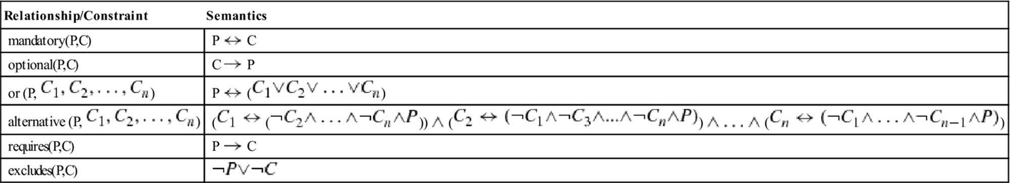
Constraints of a feature model represent restrictions that have to hold between the features. Constraint types that are typically supported by feature model languages are the following (Kang et al., 1990):

• Requires: A requires constraint between two features ( requires ) denotes the fact that if feature is included in the configuration, feature must be included as well. For example, if a Camera is included in a configuration, a high-resolution Screen must be included as well.

• Excludes: An excludes constraint between two features ( excludes ) denotes the fact that both and must not be part of the same configuration. For example, Basic Screen must not be combined with GPS.

For further discussions of feature model representations refer to Benavides et al. (2010).

Mobile Phone Configuration (Solution)

A configuration (solution) for a configuration task defined by a feature model and a corresponding set of customer requirementsis represented by a list of features and an indication for each feature whether it is active or inactive. An example mobile phone configuration was already determined by the static constraint-based approach discussed in Subsection 6.2.1.

Semantics of Feature Models

The semantics of feature models can be defined using the static constraint representation introduced in Subsection 6.2.1. If we want to express the optional relationship between Mobile Phones and GPS, we can express this relationship in terms of the constraint GPS Mobile Phones. If our goal is to translate a feature model into a static CSP representation, the rules depicted in Table 6.1 can be applied. In this definition, represents the higher-level feature and a lower-level feature that has a relationship to .

Table 6.1

Semantics of feature models defined in terms of constraints (propositional logic). Features are represented by Boolean variables.

Solution search for feature models can be implemented on the basic algorithms that are able to solve static constraint satisfaction problems (SCSPs) or satisfiability (SAT) problems.

6.3.2 UML Configuration Models

We now introduce a UML-based configuration knowledge representation¹³ that can also be used in complex domains where size and structure of configurations are unknown beforehand. In this context, we introduce a configuration model of personal computers (PCs), which is used as a working example in this book. It consists of two major parts: (1) The basic structure of a PC is represented in terms of a partonomy with associated generalization hierarchies (see Figure 6.7) and (2) additional constraints that restrict the combination of individual components. Some basic constraints () are directly integrated in the configuration model of Figure 6.7; the remaining ones () are introduced textually in Table 6.2.¹⁴ The modeling facilities introduced in the following can be seen as major concepts needed for the design of a configuration model (Falkner and Haselböck, 2013; Felfernig, 2007; Felfernig et al., 2000a, 2001, 2003; Soininen et al., 1998). For the representation of configuration models in UML we rely on the notation of class diagrams; no further notations such as component diagrams or sequence diagrams are needed in this context.

Table 6.2

Constraints related to the configuration model shown in Figure 6.7.

The major motivation for applying UML notations for configuration modeling is that the language is a de facto software engineering industry standard and thus more easily accessible for the stakeholders in a development project. Furthermore, it can be directly translated into predicate logic (Falkner and Haselböck, 2013; Felfernig, 2007; Felfernig et al., 2000a, 2003). For a discussion of a UML-based configurator application development process refer to Friedrich et al. (2014)¹⁵.

Computer Configuration Model in UML: Structure

In a configuration model (see Figure 6.7), the structure of a configurable product is defined on the basis of the modeling facilities component types (concepts or classes), associations with multiplicities, and generalizations. Note that existing commercial configuration environments do not directly support UML-based representations but typically include similar modeling facilities that allow the representation of partonomies, generalization hierarchies, and constraints.

• Component types: A component type has a unique name and is characterized by a set of attributes. Attributes are defined on the basis of datatypes (the datatype of each attribute is defined in [datatype], which can denote a constant, an enumeration, or a range). For example, maxprice[0..2500] specifies an integer range attribute of the component type PC. In the examples in this book, attributes are single-valued; that is, no attribute has more than one value.

• Associations and Multiplicities: The part-of modeling facility is used to describe part-of associations between component types. In its simplest form, these associations are assumed to be of type composite (not shared); this means that no instance (component) of a component type can be part of more than one instance (whole component). For example, each CPU is part of exactly one MB (motherboard) and each MB consists of one or two CPUs. Note that we apply multiplicities to further describe associations between component types. Other examples of multiplicities are the following: each PC (personal computer) consists of one or more Applications (no upper limit defined here) and each Application is part of exactly one PC. Each harddisk (HDisk) has exactly one DiskPort and eachDiskPort is associated with one HDisk (within the same HDUnit). Furthermore, each DiskPort is connected with a ControllerPort. Note that additional types of associations are included in the individual book chapters where needed.

• Generalizations: This modeling facility relates two or more component types through a subset relation. The generalization relationship between subtypes and supertype (or the inverse specialization relationship between supertype and subtypes) can be characterized as disjoint and complete. Disjointness means that each instance of a component type X can be assigned to only one of the subtypes of X. For example, each CPU is either of type CPUS or CPUD but not both. Completeness means that each instance is assigned to one of the leaf nodes of the generalization hierarchy. Furthermore, generalization hierarchies in the configuration context typically do not allow multiple inheritance. Again, further modeling facilities with different semantics are introduced in the other chapters of this book where needed. Note that for reasons of simplicity no definition of specific application types is included in our example; it is assumed that each instance of type Application has the same required hdcapacity (200) and the same price, which is 50. In a complete model of a personal computer additional subtypes would be included or defined as part of a corresponding component catalog.

Computer Configuration Model in UML: Constraints

Constraints represent restrictions that have to hold between attributes and/or component types. Constraints frequently used in configuration models are now explained on the basis of our PC configuration model (see Table 6.2).¹⁶

We differentiate between the following types of constraints: (1) Constraints that are directly integrated into the configuration model depicted in Figure 6.7 are denoted as graphical constraints (). (2) Constraints regarding the pricing of a configurable product can be defined as part of the configuration model. In many real-world scenarios pricing constraints (policies) are not part of the configuration model but rather implemented as a separate pricing component. We denote the set of pricing constraints as . (3) Constraints restricting the production and consumption of resources are denoted as resource constraints (). (4) Constraints that define in which context which additional components have to be part of a configuration (solution) are denoted as requires constraints (). Requires constraints {–} are defined in addition to the ones already contained in . (5) Restrictions regarding the way in which different components (instances of component types) can be combined with each other are defined on the basis of compatibility constraints (). The compatibility constraints {–} are defined in addition to the ones already contained in . The graphical constraint describes an incompatibility, which is the complement of a compatibility. Compatibilities are used in cases where the number of allowed combinations of components (or attribute values) is low. Alternatively, if the number of incompatibilities is low, incompatibility constraints are used. Quite often, the term compatibility constraint denotes both compatibilities and incompatibilities. All the constraints of the configuration model ¹⁷ together with a set of customer requirements are major elements of a configuration task that can be solved by a configurator (configuration system).

Computer Configuration (Solution)

A configuration (solution to a configuration task) can be represented as a UML instance diagram; an example of such a diagram is depicted in Figure 6.8. The diagram depicts concrete components (instances of the classes depicted in the configuration model ofFigure 6.7).

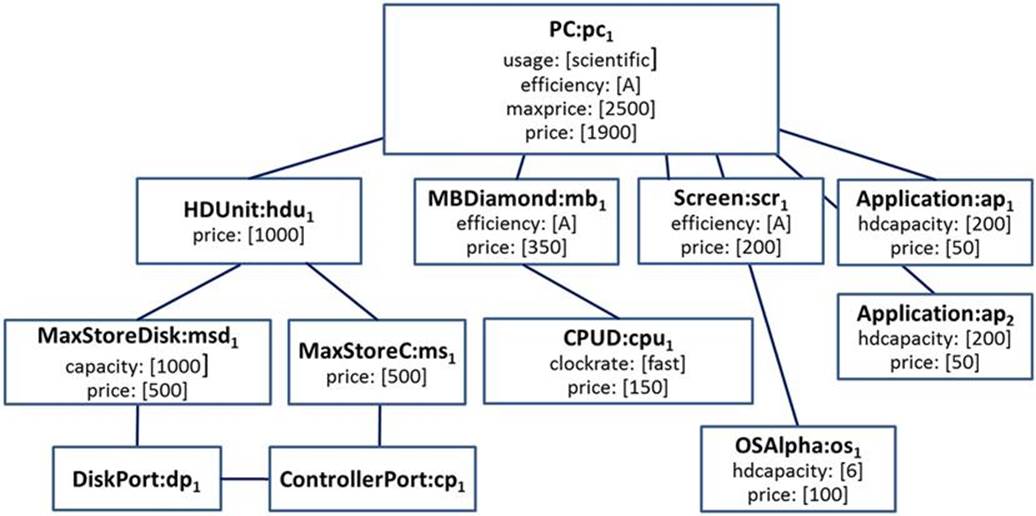
FIGURE 6.8 Configuration (solution) depicted as a UML instance diagram.

6.4 Logic-Based Knowledge Representation

6.4.1 First Order Logic (FOL)

The semantics of UML modeling facilities is explained on the basis of the configuration model depicted in Figure 6.9. This is a fragment of our PC configuration model of Figure 6.7, which includes the component types {PC, MB, MBDiamond, MBSilver, CPU, CPUS, CPUD, OS,OSAlpha, OSBeta} and the constraints {gc1, gc2, gc3, prc2’, resc1} (see Table 6.3).¹⁸ In order to define the semantics of UML-based configuration models, we will apply a decidable subset of first-order logic (FOL). This is in the line of research dedicated to the formalization of component-oriented representations (see, e.g., Falkner and Haselböck, 2013; Felfernig, 2007; Felfernig et al., 2000a, 2003; Schröder et al., 1996).

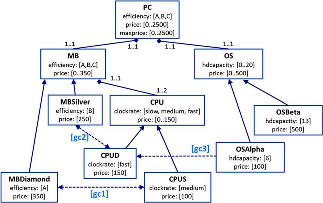
FIGURE 6.9 Fragment of the PC model adapted part of Figure 6.7.

Table 6.3

Constraints related to the configuration model in Figure 6.9.

Configuration Task and Solution

We will now introduce a predicate logic-based definition of a configuration task (problem) and its solution, which is used in the remaining sections of this chapter. This definition is based on Felfernig et al. (2004, 2003). From now on we concentrate on a generalized (component-oriented) knowledge representation based on component types and generic constraints (similar to the concepts also provided by generative constraint satisfaction approaches; Mailharro, 1998; Stumptner et al., 1998).

Definition

Configuration Task

A configuration task can be defined as a triple () where and are sets of logical sentences and is a set of predicate symbols. represents the configuration model and specifies particular system (customer) requirements. A configuration is described by a set of positive ground literals whose predicate symbols are in .

Definition

Configuration (Solution)

Given a configuration task (), a configuration is consistent if and only if is satisfiable. A configuration is valid if it is consistent and a set of completeness axioms related to is fulfilled. together with the corresponding completeness axioms is denoted as .

In order to be able to guarantee the completeness property, we have to introduce an additional formula for each of the predicate symbols in —the so-called completeness axioms (; Felfernig et al., 2004). These axioms help to deduce the negation of all possible instances of literals whose predicate symbols are in with the exception of the positive ground literals contained in ; that is, all instances of predicates not explicitly described in are negated (for an example see Table 6.6). This process is also known as Clark Completion (see Russel and Norvig, 2003).

Table 6.4

Example formalizations of the model () depicted in Figure 6.9. getcpus denotes a collection operator (Felfernig et al., 2000a) that collects all connected with motherboard . For reasons of readability we limit the example to attribute range restrictions (e.g., PC(efficiency)).

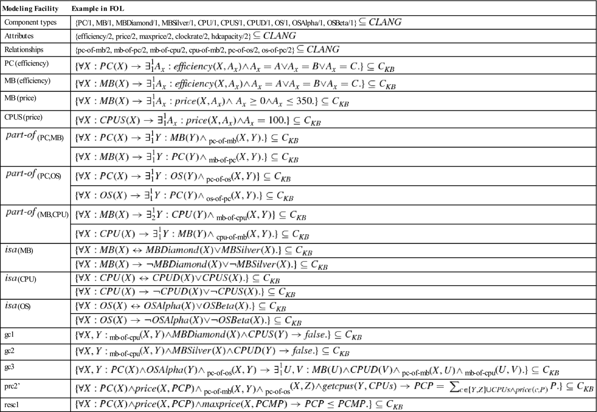
Table 6.5

Example representation of user (customer) requirements(REQ).

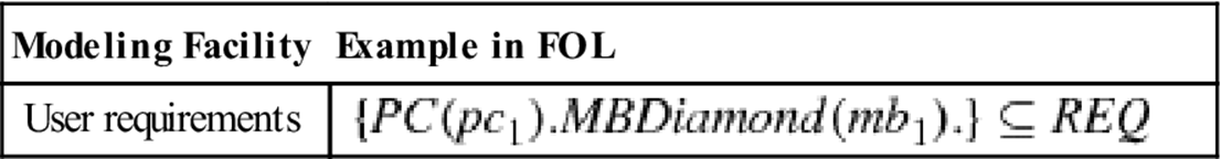
Table 6.6

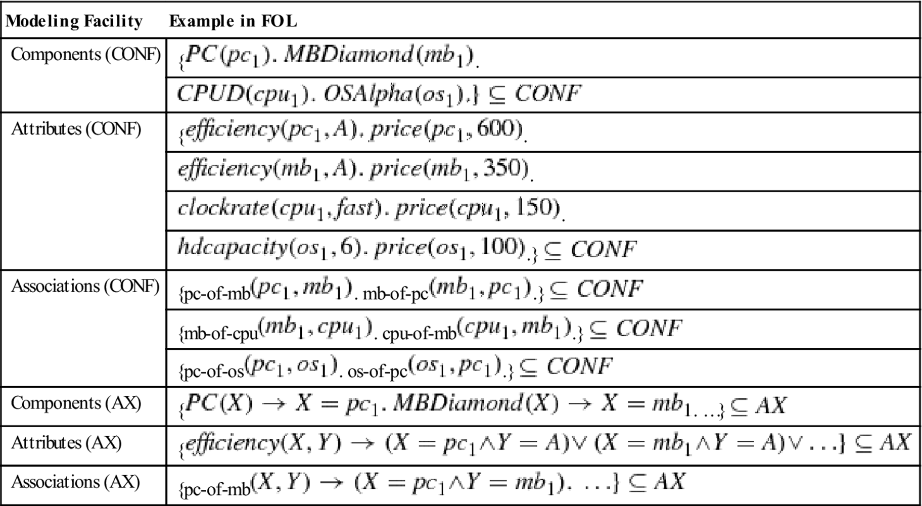
Example configuration (CONF) with completeness axioms (AX).

Semantics of UML Configuration Models

The first step in formalizing a configuration model is to define the needed component types, attributes, and relationships in terms of FOL unary and binary predicates (see Table 6.4).

For each attribute, we have to restrict the allowed attribute values in the context of a certain class. For example, the price of a MB can have a value between and whereas the price of a CPUS is restricted to the value of . Thereafter, we define the part-ofrelationships between component types; in Table 6.4 this is exemplified on the basis of the part-of relationship between MB and CPU. The semantics of generalization (isa) hierarchies is assumed to be disjoint and complete. For example, each MB is either an MBDiamond or anMBSilver. At the same time, a motherboard cannot be both an MBDiamond and an MBSilver. All rules for translating UML configuration models into a corresponding logic-based representation can be found in Felfernig (2007), and Felfernig et al. (2000a, 2003).

In order to specify a configuration task we also need to define a set of customer requirements (). These are represented as facts that have to be taken into account by the configurator (see Table 6.5).

Computer Configuration (Solution) in FOL

A configuration can be interpreted as an assignment to all the decision points that are specified in the configuration model. Such an assignment is complete if all decision points are instantiated; it is consistent if all the constraints in are fulfilled. Finally, the assignment is valid if it is consistent and complete. A solution to the configuration task defined by our example is shown in Table 6.6.

6.4.2 Logic-Based Configuration

We used FOL to specify the semantics of modeling concepts that can be used for the development of a configuration model. In this section, we introduce logic-based approaches, which can be applied to solve a configuration task to calculate a solution (configuration).

Answer Set Programming

Answer Set Programming (ASP) emerged in the late 1990s as an approach to the declarative modeling and solving of computational problems. The paradigm is a result of intensive research in the areas of knowledge representation, deductive databases, and logic programming (Brewka et al., 2011). ASP is a subset of FOL interpreted under stable-model semantics (Gelfond and Lifschitz, 1988). It is worth mentioning that configuration was one of the first real-world applications of ASP (see Soininen et al., 2001; Tiihonen et al., 2003, 2013). ASP programs are represented as a finite set of rules where (head of the rule), and (body of the rule) are classical FOL atoms. In a rule, the atom in the head is true if all literals of the body are true; that is, there is a derivation for each positive literal whereas none of the negative literals can be derived.

A rule with an empty head (placeholder for false) is denoted as integrity constraint. For example, . denotes the incompatibility between the component types MBDiamond and CPUS (see Figure 6.9). A rule with an empty body is denoted as fact; for example, denotes the two facts and . Finally, weight constraints allow the definition of choices. For example, denotes the fact that between 1 and 2 CPUs can be included in a configuration (cpu_domain describes the available CPU instances). The determination of configurations for ASP programs is based on two steps: (1) first order variables of the program are systematically replaced by the elements of the Herbrand universe (this process is also denoted as grounding (e.g., Gebser et al., 2009)) and (2) the resulting (variable-free) program is then fed into the ASP solver that determines stable models (answer sets), minimal models of the ASP program (Giunchiglia et al., 2006). The ASP representation of the configuration model depicted in Figure 6.9 is shown in Table 6.7. For reasons of readability we omitted the specification of attribute domains on all levels of the generalization hierarchy. For example, the specification of the possible values of theclockrate attribute (component type cpu) can be implemented as follows: 1{clockrate(C,A): clockrate_domain(A)}1 :- cpu(C). clockrate_domain(slow;medium;fast). ASP representations of customer requirements and a configuration result are shown in Table 6.8.

Table 6.7

Example formalizations of the PC configuration model shown in Figure 6.9 defined in clingo (see potassco.sourceforge.net).

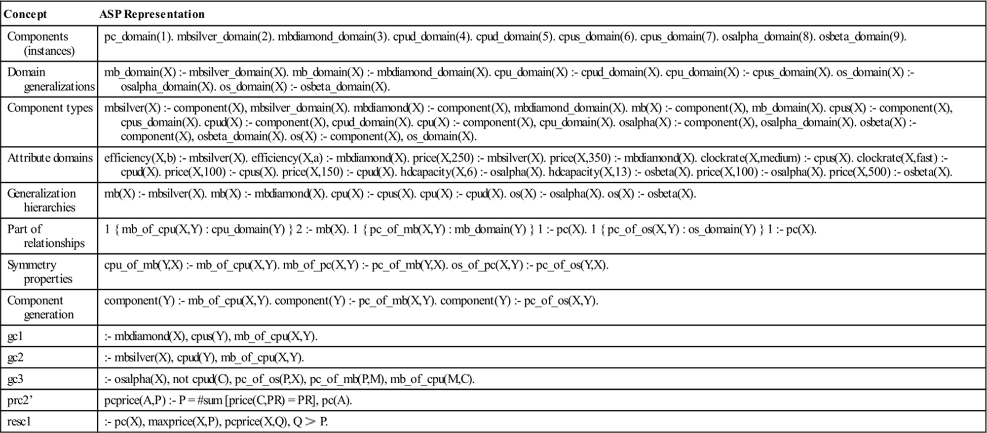
Table 6.8

Example configuration result calculated by clingo (see potassco.sourceforge.net).

Description Logics

Description Logics (DL; Baader et al., 2003) is a popular knowledge representation formalism in the context of the Semantic Web. DL can be used for configuration knowledge representation, especially for the design of component type hierarchies (ontologies) and for coherence analysis. A Description Logic knowledge base consists of two major elements: the introduces concepts, relationships, and constraints of the (product) domain, the contains assertions about individuals. Thus, the TBox can be used to represent the configuration model and the ABox the resulting configuration. Description Logics have been successfully applied for the development of configuration systems—for a detailed related discussion refer to Hotz et al. (2006) and McGuinness and Wright (1998).Felfernig et al. (2003) have analyzed the applicability of Description Logics for the representation of configuration knowledge. DL can be used to represent configuration knowledge, however, some specific constraint types are supported in a restricted fashion. For example, no aggregation functions are provided and constraints on complex connection structures (via ports) cannot be defined due to the lower (but decidable) expressiveness of many DL dialects. Furthermore, because there is no standard inference method that provides automatic instantiation, the DL-Reasoner has to be included in an architecture that creates individuals from outside. This is needed because of the incremental aspects of configuration processes (see Buchheit et al., 1995; Hotz and Neumann, 2005;Stumptner, 1997). Beside this analysis, Felfernig et al. (2003) also introduce a formal definition of a configuration problem and its solution in Description Logic and show the equivalence of this definition with a predicate logic-based definition.

Hybrid Configuration

Hybrid configuration exploits several representation and reasoning mechanisms (Stumptner, 1997). Typically, there is an ontology-like (DL-based) representation (Baader et al., 2003) for representing components, their compositional relations, and attributes. Additionally, constraints are used for representing n-ary relations between components and for computing and inferring attribute values. The configuration process combines the related inference mechanisms, ontology inference services, and constraint propagation in a cyclic manner. Additionally, procedural knowledge (Hotz et al., 2006; McDermott, 1982) can be used for describing the order of configuration steps of the configuration process. A detailed description of a configuration environment based on a hybrid configuration approach is given in Hotz and Günter (2014)¹⁹.

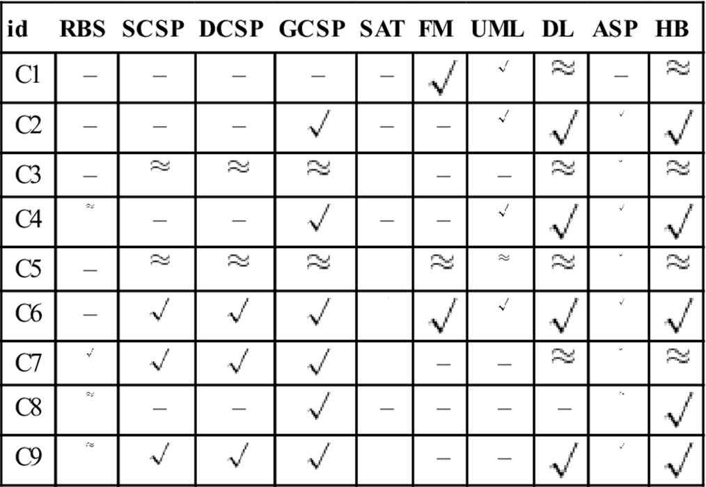
6.5 Comparison of Knowledge Representations

We now compare the configuration knowledge representations that have been discussed within the scope of this chapter (RBS rule-based systems, SCSP static constraint satisfaction, DCSP dynamic constraint satisfaction, GCSP generative constraint satisfaction, SAT SAT solving, FM feature models, UML UML configuration models, DL Description Logics, ASP Answer Set Programming, HB hybrid configuration).We will first provide an overview of the relevant criteria (see Table 6.9) and then discuss the evaluation results (see Table 6.10).

Table 6.9

Criteria for comparing configuration knowledge representations.

Table 6.10

Evaluation of representations (RBS = rule-based systems, SCSP = static CSP, DCSP = dynamic CSP, GCSP = generative CSP, SAT = Sat Solving, FM = feature models, UML = UML configuration models, DL = Description Logics, ASP = Answer Set Programming, HB = hybrid configuration). = good support, = some support, and – = no support.

6.5.1 Evaluation Criteria

The evaluation criteria are summarized in Table 6.9. The first evaluation criterion () is related to the availability of standard graphical modeling concepts that help (1) to improve the understandability of configuration knowledge and (2) to increase the efficiency of configuration knowledge base development and maintenance processes. Criterion is related to the question whether the knowledge representation formalism supports configuration knowledge design on the basis of concepts near to real-world entities (i.e., component types, attributes, relationships, generalization hierarchies, relevant constraint types, etc.). raises the question whether mechanisms for automated consistency maintenance are available; for example, if a new constraint (or concept) is added to the knowledge base, it should be immediately clear, whether inconsistencies are introduced or not. Criterion is related to the availability of modularization and structuring concepts for knowledge bases; for example, in which way is it possible to organize (group) the constraints inside a knowledge base. evaluates the quality of support of knowledge base evolution and maintenance, for example, in terms of intelligent navigation support in complex knowledge spaces. evaluates whether the underlying knowledge representation is model-based. poses the question whether the type of knowledge representation allows efficient reasoning. evaluates whether a generative configuration scenario can be implemented; that is, whether components and related constraints can be generated on-demand (see Subsection 6.2.2). is related to the question whether the generation of explanations can be supported.

6.5.2 Comparison of Knowledge Representations

On the basis of the evaluation criteria summarized in Table 6.9 we are able to discuss the advantages and disadvantages of the knowledge representation formalisms presented in this chapter (see Table 6.10).

These formalisms are evaluated on the basis of criteria on a rating scale of (= good support, = some support, and – = no support). Standard graphical knowledge representations () are primarily provided by feature models (Benavides et al., 2010) and component-oriented modeling approaches such as the Unified Modeling Language (Felfernig, 2007; Felfernig et al., 2000a). Component-oriented modeling () is supported by GCSPs (Stumptner et al., 1998) and modeling approaches in the line of UML, Description Logics (Baader et al., 2003), Answer Set Programming (ASP; Brewka et al., 2011), and Hybrid Configuration (HB; Stumptner, 1997). Automated consistency maintenance () can easily be implemented on top of most of the given knowledge representations (Felfernig et al., 2004, 2012). FM and UML artifacts have to be connected with a corresponding reasoning support. Intelligent modularization () in GCSP, UML, DL, and HB is supported in terms of a component (class) dependent definition of domain constraints. With the exception of RBS all representations allow an arbitrary ordering (organization) of the constraints in the knowledge base without changing its underlying semantics; RBS often also dispose of concepts for structured rule representation. Graphical UML modeling supports the inclusion of advanced modularization concepts such as packaging and diagram contextualization (Felfernig et al., 2000b; Felfernig and Zanker, 2000). Techniques for easy knowledge base evolution and maintenance () are not primarily depending on the knowledge representation itself but more on additional meta-functionalities that support intuitive knowledge navigation and adaptation; nearly all representation formalisms can be equipped with such a functionality (Felfernig et al., 2013b). RBS have serious maintenance problems due to the dependence of product domain and problem solving knowledge. With the exception of RBS, all other representations follow a model-based paradigm () that supports a clear separation of domain and problem-solving knowledge. RBS and constraint satisfaction algorithms have proven to support efficient problem solving on an industrial scale. For this reason, these approaches are evaluated better with regard to performance (). GCSP allows the determination of solutions for generative configuration problems; ASP and HB are also able to provide such functionalities (). With the exception of FM and UML, all approaches provide basic support for explanations (as to why a configuration could (not) be found). Dependencies between domain and problem solving knowledge in RBS and encodings in SAT (see Subsection 6.2.1) make these approaches less accessible for explanation techniques.

6.6 Conclusion

In this chapter we provided an overview of different configuration knowledge representation and reasoning techniques. These techniques were discussed on the basis of a timeline ranging from the rule-based configuration system R1/XCONimplemented in the late 1970’s via different types of constraint representations and constraint reasoning approaches through to advanced knowledge representation and reasoning approaches that are applied nowadays for the definition and solution of configuration tasks.

References

1. Amilhastre J, Fargier H, Marquis P. Consistency restoration and explanations in dynamic CSPs - application to configuration. Artificial Intelligence. 2002;135(1–2):199–234.

2. Andersen H, Hadzic T, Pisinger D. Interactive cost configuration over decision diagrams. Journal of Artificial Intelligence Research. 2010;37:99–139.

3. Baader F, Calvanese D, McGuinness DL, Nardi D, Patel-Schneider PF, eds. The Description Logic Handbook: Theory, Implementation, and Applications. New York, NY: Cambridge University Press; 2003.

4. Bacchus F, vanBeek P. On the conversion between non-binary and binary constraint satisfaction problems. In: 15th National Conference on Artificial Intelligence (AAAI’98) Madison, Wisconsin. 1998:311–318.

5. Batory D. Feature models, grammars, and propositional formulas. In: Obbink H, Pohl K, eds. Software Product Lines Conference. Rennes, France: Springer; 2005:7–20. Lecture Notes in Computer Science vol. 3714.

6. Benavides D, Segura S, Ruiz-Cortés A. Automated analysis of feature models 20 years later: a literature review. Information Systems. 2010;35(6):615–636.

7. Booch G, Rumbaugh J, Jacobson I. Unified Modeling Language User Guide. second ed Reading, MA: Addison-Wesley; 2005.

8. Bowen J, Bahler D. Conditional existence of variables in generalized constraint networks. In: 9th National Conference on Artificial Intelligence (AAAI-91) Anaheim, California. 1991:215–220.

9. Brailsford S, Potts C, Smith B. Constraint satisfaction problems: algorithms and applications. European Journal of Operational Research. 1999;199(3):557–581.

10. Brewka G, Eiter T, Truszczyński M. Answer set programming at a glance. Communications of the ACM. 2011;54(12):92–103.

11. Buchheit, M., Klein, R., Nutt, W., 1995. Constructive Problem Solving: A Model Construction Approach Towards Configuration, Deutsches Forschungszentrum für Künstliche Intelligenz, Saarbrücken (TM-95-01).

12. Claessen K, Een N, Sheeran M, Sörensson N. SAT-solving in practice. In: 9th International Workshop on Discrete Event Systems Göteborg, Sweden. 2008:61–67.

13. Czarnecki K, Helsen S, Eisenecker U. Formalizing cardinality-based feature models and their specialization. SoftwareProcess: Improvement and Practice. 2005;10(1):7–29.

14. Falkner A, Haselböck A. Challenges of knowledge evolution in practice. AI Communications. 2013;26(1):3–14.

15. Falkner A, Schreiner H. SIEMENS: configuration and reconfiguration in industry. In: Felfernig A, Hotz L, Bagley C, Tiihonen J, eds. Knowledge-based Configuration – From Research to Business Cases. Waltham, MA: Morgan Kaufmann Publishers; 2014:199–210. (Chapter 16).

16. Falkner A, Felfernig A, Haag A. Recommendation technologies for configurable products. AI Magazine. 2011;32(3):99–108.

17. Faltings, B., Weigel, R., 1994. Constraint-based knowledge representation for configuration systems. Tech. Rep. TR-94/59, Ecole Polytechnique Fédérale de Lausanne (EPFL), Switzerland.

18. Felfernig A. Standardized configuration knowledge representations as technological foundation for mass customization. IEEE Transactions on Engineering Management. 2007;54(1):41–56.

19. Felfernig A, Burke R. Constraint-based recommender systems: technologies and research issues. In: ACM International Conference on Electronic Commerce (ICEC08) Innsbruck, Austria. 2008:17–26.

20. Felfernig A, Zanker M. Diagrammatic acquisition of functional knowledge for product configuration systems with the unified modeling language. In: Proceedings of the First International Conference on Theory and Application of Diagrams (Diagrams ’00). London, UK: Springer-Verlag; 2000:361–375. Lecture Notes in Computer Science vol. 1889.

21. Felfernig A, Friedrich GE, Jannach D. UML as domain specific language for the construction of knowledge-based configuration systems. International Journal of Software Engineering and Knowledge Engineering. 2000a;10(4):449–469.

22. Felfernig A, Jannach D, Zanker M. Contextual diagrams as structuring mechanisms for designing configuration knowledge bases in UML. In: 3rd International Conference on the Unified Modeling Language (UML2000). York, UK: Springer; 2000b:240–254. Lecture Notes in Computer Science Vol. 1939.

23. Felfernig A, Friedrich G, Jannach D. Conceptual modeling for configuration of mass-customizable products. Artificial Intelligence in Engineering. 2001;15(2):165–176.

24. Felfernig A, Friedrich G, Jannach D, Stumptner M, Zanker M. Configuration knowledge representations for semantic web applications. Artificial Intelligence for Engineering Design, Analysis and Manufacturing (AI EDAM). 2003;17(1):31–50.

25. Felfernig A, Friedrich G, Jannach D, Stumptner M. Consistency-based diagnosis of configuration knowledge bases. Artificial Intelligence. 2004;152(2):213–234.

26. Felfernig A, Schubert M, Zehentner C. An efficient diagnosis algorithm for inconsistent constraint sets. Artificial Intelligence for Engineering Design, Analysis and Manufacturing (AI EDAM). 2012;26(1):53–62.

27. Felfernig A, Benavides D, Galindo J, Reinfrank F. Towards anomaly explanation in feature models. In: Workshop on Configuration Vienna, Austria. 2013a:117–124.

28. Felfernig A, Reiterer S, Stettinger M, Reinfrank F, Jeran M, Ninaus G. Recommender systems for configuration knowledge engineering. In: Workshop on Configuration Vienna, Austria. 2013b:51–54.

29. Fleischanderl G, Friedrich GE, Haselböck A, Schreiner H, Stumptner M. Configuring large systems using generative constraint satisfaction. IEEE Intelligent Systems. 1998;13(4):59–68.

30. Freuder E. In pursuit of the holy grail. Constraints. 1997;2(1):57–61.

31. Friedrich G, Jannach D, Stumptner M, Zanker M. Knowledge engineering for configuration systems. In: Felfernig A, Hotz L, Bagley C, Tiihonen J, eds. Knowledge-based Configuration – From Research to Business Cases. Waltham, MA: Morgan Kaufmann Publishers; 2014:139–155. (Chapter 11).

32. Gebser M, Kaminski R, Ostrowski M, Schaub T, Thiele S. On the input language of ASP grounder Gringo. In: Erdem E, Lin F, Schaub T, eds. Proceedings of the 10th International Conference on Logic Programming and Nonmonotonic Reasoning. Potsdam, Germany: Springer; 2009:502–508. Lecture Notes in Computer Science Vol. 5373.

33. Gelfond M, Lifschitz V. The stable model semantics for logic programming. In: Kowalkowski RA, Bowen KA, eds. Logic Programming: Proceedings of the 5th International Conference and Symposium Seattle, WA. 1988:1070–1080.

34. Giunchiglia E, Lierler Y, Maratea M. Answer set programming based on propositional satisfiability. Journal of Automated Reasoning. 2006;36(4):345–377.

35. Gomes C, Kautz H, Sabharwal A, Selman B. Satisfiability solvers. In: Handbook of Knowledge Representation. New York, NY: Elsevier; 2008:89–134. Foundations of Artificial Intelligence vol. 3 (Chapter 2).

36. Günter A, Kühn C. Knowledge-Based Configuration - Survey and Future Directions. In: Puppe F, ed. XPS-99: knowledge based systems, proceedings 5th biannual german conference on knowledge based systems. Würzburg: Springer; 1999; Lecture Notes in Artificial Intelligence Vol. 1570.

37. Hotz L, Günter A. KONWERK. In: Felfernig A, Hotz L, Bagley C, Tiihonen J, eds. Knowledge-based Configuration – From Research to Business Cases. Waltham, MA: Morgan Kaufmann Publishers; 2014:281–295. (Chapter 24).

38. Hotz L, Neumann B. Scene Interpretation as a Configuration Task. Künstliche Intelligenz. 2005;3:59–65.

39. Hotz L, Wolter K. Smarthome Configuration Model. In: Felfernig A, Hotz L, Bagley C, Tiihonen J, eds. Knowledge-based Configuration – From Research to Business Cases. Waltham, MA: Morgan Kaufmann Publishers; 2014:121–135. (Chapter 10).

40. Hotz L, Wolter K, Krebs T, et al. Configuration in Industrial Product Families - The ConIPF Methodology. Berlin: IOS Press; 2006.

41. Jannach D, Zanker M, Felfernig A, Friedrich G. Recommender Systems: An Introduction. MA: Cambridge University Press; 2010.

42. Janota M. Do SAT solvers make good configurators? In: First Workshop on Analyses of Software Product Lines (ASPL08) of 12th International Software Product Lines Conference (SPLC08) Limerick, Ireland. 2008:10–14.

43. Janota M, Botterweck G, Grigore R, Marques-Silva J. How to complete an interactive configuration process? In: 36th Conference on Current Trends in Theory and Practice of Computer Science (SOFSEM 2010). Špindlerův Mlýn, Czech Republic: Springer; 2010;528–539. Lecture Notes in Computer Science vol. 5901.

44. Jüngst W, Heinrich M. Using resource balancing to configure modular systems. IEEE Intelligent Systems. 1998;13(4):50–58.

45. Junker U. QUICKXPLAIN: preferred explanations and relaxations for over-constrained problems. In: McGuinness DL, Ferguson G, eds. 19th Intl Conference on Artifical Intelligence (AAAI’04). AAAI Press 2004:167–172.

46. Junker U. Configuration. In: Rossi F, vanBeek P, Walsh T, eds. Handbook of Constraint Programming. New York, NY: Elsevier; 2006:837–873. Foundations of Artificial Intelligence vol. 2.

47. Junker U, Mailharro D. The logic of ILOG (J)Configurator: Combining constraint programming with a description logic. In: 18th International Joint Conference on Artificial Intelligence (IJCAI-03), Configuration Workshop Acapulco, Mexico. 2003:13–20.

48. Kang, K., Cohen, S., Hess, J., Novak, W., Peterson, S., 1990. Feature-Oriented Domain Analysis Feasibility Study (FODA). Tech. Rep. CMU/SEI-90-TR-021, Carnegie Mellon University, Software Engineering Institute, Pittsburgh, PA.

49. Kiziltan Z, Hnich B. Symmetry breaking in a rack configuration problem. In: Seventeenth International Joint Conference on Artificial Intelligence (IJCAI-2001), Workshop on Modelling and Solving Problems with Constraints Seattle, WA. 2001;1–6.

50. Leitner G, Felfernig A, Blazek P, Reinfrank F, Ninaus G. User interfaces for configuration environments. In: Felfernig A, Hotz L, Bagley C, Tiihonen J, eds. Knowledge-based Configuration – From Research to Business Cases. Waltham, MA: Morgan Kaufmann Publishers; 2014:89–106. (Chapter 8).

51. Li B, Chen L, Huang Z, Zhong Y. Product configuration optimization using a multiobjective genetic algorithm. International Journal of Advanced Manufacturing Technology. 2006;30(1–2):20–29.

52. Mackworth A. Consistency in networks of relations. Artificial Intelligence. 1977;8(1):99–118.

53. Mailharro D. A classification and constraint-based framework for configuration. Artificial Intelligence for Engineering Design, Analysis and Manufacturing (AI EDAM). 1998;12(4):383–397.

54. McDermott J. R1: a rule-based configurer of computer systems. Artificial Intelligence. 1982;19(1):39–88.

55. McGuinness D, Wright J. An industrial-strength description logic-based configurator platform. Intelligent Systems and their Applications, IEEE. 1998;13(4):69–77.

56. Mittal S, Falkenhainer B. Dynamic constraint satisfaction problems. In: Proceedings of the eighth national conference on artificial intelligence (AAAI-90) Boston, MA. 1990:25–32. Aug.

57. Mittal S, Frayman F. Towards a generic model of configuration tasks. In: 1989:1395–1401. 11th International Joint Conference on Artificial Intelligence (IJCAI-89) Detroit, Michigan. vol. 2.

58. Neumann B. Configuration expert systems: a case study and tutorial. In: Bunke HO, ed. Proc 1988 SGAICO Conference on Artificial Intelligence in Manufacturing, Assembly, and Robotics Oldenbourg, Munich. 1988;27–68.

59. Pinedo M. Scheduling: Theory, Algorithms, and Systems. fourth ed New York, NY: Springer; 2012.

60. Pitiot P, Aldanondo M, Vareilles E, Gaborit P, Djefel MSC. Concurrent product configuration and process planning, towards an approach combining interactivity and optimality. International Journal of Production Research. 2013;51(2):524–541.

61. Puget J-F, Albert P. PECOS: programmation par contraintes orientée objets. Génie logiciel et systèmes experts (GLSE). 1991;23:100–105.

62. Reiter R. A theory of diagnosis from first principles. Artificial Intelligence. 1987;32(1):57–95.

63. Rossi F, vanBeek P, Walsh T, eds. Handbook of Constraint Programming Foundations of Artificial Intelligence. New York, NY: Elsevier; 2006.

64. Russel S, Norvig P. Artificial Intelligence – A Modern Approach. 2nd Edition Upper Saddle River, NJ: Prentice Hall; 2003.

65. Sabin D, Weigel R. Product configuration frameworks – a survey. IEEE Intelligent Systems. 1998;13(4):42–49.

66. Schröder C, Möller R, Lutz C. A partial logical reconstruction of PLAKON/KONWERK. In: Baader F, Bürckert H-J, Günther A, Nutt W, eds. Proceedings of the Workshop on Knowledge Representation and Configuration WRKP’96 No D-96-04 in DFKI Documents. 1996:55–64.

67. Sinz, C., Haag, A., Narodytska, N., Walsh, T., Gelle, E., Sabin, M., Junker, U., O’Sullivan, B., Rabiser, R., Dhungana, D., Grünbacher, P., Lehner, K., Federspiel, C., Naus, D., 2007. Configuration. IEEE Intelligent Systems 22 (1), 78–90.

68. Soininen T, Tiihonen J, Männistö T, Sulonen R. Towards a general ontology of configuration. Artificial Intelligence for Engineering Design, Analysis and Manufacturing (AI EDAM). 1998;12(4):357–372.

69. Soininen, T., Niemelä, I., Tiihonen, J., Sulonen, R., 2001. Representing configuration knowledge with weight constraint rules. In: Provetti, A., Son, T.C. (Eds.), 1st International Workshop on Answer Set Programming: Towards Efficient and Scalable Knowledge (AAAI Technical, Report SS-01-01). pp. 195–201.

70. Soloway E, Bachant J, Jensen K. Assessing the maintainability of XCON-in-RIME: coping with the problem of very large rule-bases. In: Proceedings of the Sixth National Conference on Artificial Intelligence (AAAI-87) Seattle, Washington. 1987:824–829. July 13–17.

71. Stumptner M. An overview of knowledge-based configuration. AI Communications. 1997;10(2):111–126.

72. Stumptner M, Friedrich G, Haselböck A. Generative constraint-based configuration of large technical systems. Artificial Intelligence for Engineering Design, Analysis and Manufacturing (AI EDAM). 1998;12(4):307–320.

73. Terashima-Marin H, Ross P, Valenzuela-Rendon M. Hyper-heuristics for the dynamic variable ordering in constraint satisfaction problems. In: Genetic and Evolutionary Computation Conference (GECCO’08) Atlanta, Georgia. 2008:571–578.

74. Tiihonen J, Soininen T, Niemelä I, Sulonen R. A practical tool for mass-customising configurable products. In: Proceedings of the 14th International Conference on Engineering Design, Stockholm, Sweden, August 19–21, 2003, CDROM. 2003; p. 10 (Paper number: 1290).

75. Tiihonen J, Heiskala M, Anderson A, Soininen T. WeCoTin – A practical logic-based sales configurator. AI Communications. 2013;26(1):99–131.

76. Tsang E. Foundations of Constraint Satisfaction. London, San Diego, New York: Academic Press; 1993.

77. Warmer J, Kleppe A. The Object Constraint Language: Getting Your Models Ready for MDA. second ed Boston, MA: Addison-Wesley Longman Publishing; 2003.