The Profitable Supply Chain: A Practitioner’s Guide (2015)
Chapter 2. Inventory Planning
Goods-producing companies hold inventory to fulfill orders or in anticipation of customer demand. Indeed, inventory is reported as an asset on the balance sheet, so a company’s executives may approve holding high inventory levels in order to meet its obligations. However, in a challenging business environment where products are frequently discounted or discontinued, holding inventory has become increasingly detrimental to operational performance.
A company often maintains inventory levels based on simple rules in order to ensure availability, but with no consideration given to impact on margins. Textbooks provide some approaches toward analyzing inventory margins, but the mathematical models are often too rudimentary to be applied to typical business situations. This chapter provides a comprehensive approach toward analyzing and managing inventory situations, including the inventory-planning procedure and mathematical models for analyzing margins. Several examples are provided to help clarify how these models can be applied to practical situations.
The chapter begins with a detailed review of the role of inventory in operations and an activity-based categorization of inventory. Following this, mathematical models for analyzing inventory levels are developed for each of these categories. The chapter concludes by applying these models to analyze various business situations, illustrated via numerical examples using spreadsheets.
The Role of Inventory in Operations
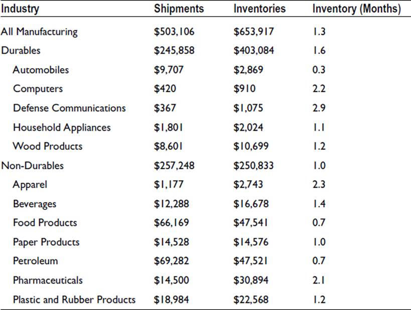
The importance of maintaining inventories can be seen from the U.S. Census Bureau’s survey of Manufacturer’s Shipments and Inventories (see Table 2-1). An electronics manufacturer is continually driving down inventory levels due to the risk of price erosion and obsolescence, while an apparel manufacturer might choose to maintain higher inventories to ensure adequate service levels. Additionally, inventory policies can vary by product within an industry—the same apparel manufacturer may hold lesser inventory of seasonal or fashion-oriented garments. As expected, electronics manufacturers maintain low inventories, mainly due to rapid price erosion. On the other hand, pharmaceuticals manufacturers maintain far higher inventory levels since there are fewer concerns related to price erosion and obsolescence.
Table 2-1. Manufacturer’s Shipments and Inventory Data (in Million USD). Source: US Census Bureau, August, 2014
Here are some common reasons for holding inventory:
· To protect against that possibility of missed revenue if demand is higher than anticipated.
· To ensure that the lack of availability of supplies in a timely manner does not result in missed demand.
· To take advantage of quantity discounts, and in anticipation of price increases.
· To negotiate seasonal demand and smooth production schedules.
· To prepare for an industry-wide shortage of raw materials or critical parts.
However, holding inventory above the immediate needs of a company has a negative aspect in the form of additional costs. These are represented as holding costs, which includes the cost of storage and handling, the cost due to tying up capital, as well as the possibility of theft, damage, and obsolescence. Therefore, the whole effort related to optimizing inventory revolves around balancing the benefits of inventory against these costs. A few of the questions that need to be addressed by inventory management, keeping this trade-off in mind, include:
· What is the inventory level required to ensure a particular level of service to the customer?
· What is the quantity that needs to be ordered for a particular product or part? How should these quantities be phased over time?
· How should inventory levels be set in order to minimize transportation, manufacturing, and purchasing costs?
· How do supplier lead times and commitment windows affect inventory policy?
· How should inventory policies be set for seasonal and lifecycle products?
· How should inventory be staged across the distribution network to maximize return on investment?
· How should part inventory levels be determined when the part is used across many different products?
These questions can arise at several different stages in the supply chain, within and across companies, as shown in Figure 2-1 and Figure 2-2. The figures list common inventory categories based on the progression of material and products through the supply chain. Comparing the two figures reveals that several inventory-related questions are common for the two supply chains, even though the products and sales models are very different. The most common inventory categories are the following:
· Cycle stock is the inventory required to meet the expected demand until the next replenishment occurs, where the expected demand is a combination of firm orders and forecasts. Since cycle stock does not account for the unexpected, safety stock (or buffer inventory) is the inventory required to account for uncertainty in demand and supply variability.
· Batch inventory is the quantity required in order to minimize transportation, manufacturing, and purchasing costs. For transportation, this includes supplies required to take advantage of full container or truckloads. For manufacturing, this includes any additional production required to minimize setup and run costs. For purchasing, this includes the additional supplies required to take advantage of price discounts.
· Seasonal or prebuild inventory refers to the accumulation of inventory due to capacity constraints at manufacturing plants. Hedge or stockpile inventory refers to any additional purchases made in anticipation of an industry-wide scarcity or price hike.
· Staged inventory refers to inventory at a distribution center that is not used to service customer demand directly, but instead used to service regional (localized) distribution centers.
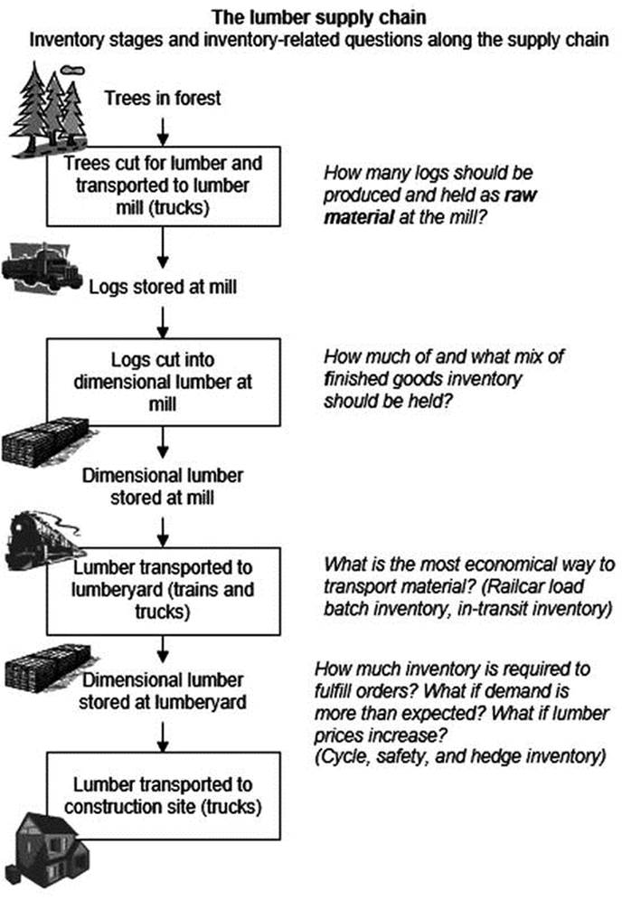
Figure 2-1. Inventories in a lumber supply chain
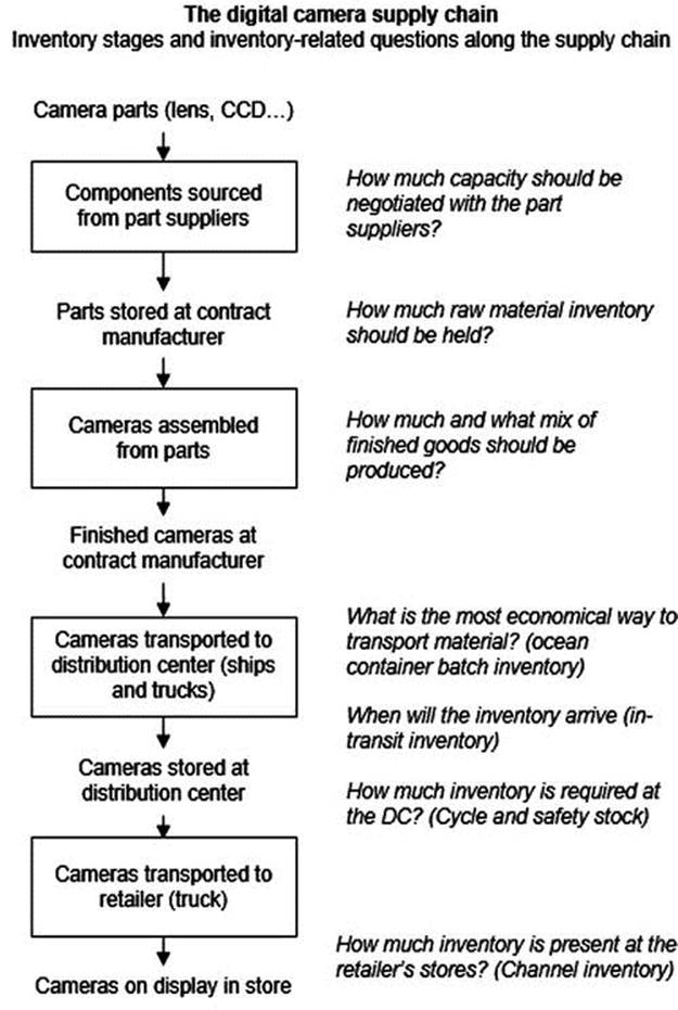
Figure 2-2. Inventories in a camera supply chain
These inventory categories are applicable to finished goods as well as raw material inventory. For a business, inventory simultaneously represents a benefit and a risk—the benefit obtained from holding inventory and quickly fulfilling orders is offset by the possibility of tying up capital and risking obsolescence. Some of these risks and trade-offs are schematized in Table 2-2. On account of this two-sided nature of inventory, it is necessary to analyze business situations carefully in order to ensure that inventory levels are frequently adjusted as changes occur. The methods and tools for determining the optimal response for different situations are described in the remaining sections of this chapter.
Table 2-2. Examples of Benefits and Drawbacks of Different Inventory Categories
|
Category |
Benefits |
Drawbacks |
|
Safety stock |
Reduces stockout and improves customer service. |
Increases inventory levels, holding costs, obsolescence risk. |
|
Batch inventory |
Reduces manufacturing and transportation costs. |
Increases inventory levels and associated costs. |
|
Seasonal inventory |
Reduces manufacturing costs (overtime) and tooling investment. |
Increases inventory-related costs since material is produced well in advance. Poor forecast accuracy can exacerbate issues. |
|
Stockpile inventory |
Improves material availability and purchase prices during industry-wide shortages. |
Increases inventory-related costs since materials are procured in advance. |
|
Staged inventory |
Reduces inventory levels while maintaining customer service levels. |
Increases facility costs due to additional storage locations. |
The Inventory Planning Process
In most companies, the responsibility for inventory management belongs to the supply chain organization. If the company does not have a separate supply chain department, this responsibility may belong to manufacturing, procurement, or distribution, depending on the company’s heritage. In all situations, it is important to identify a single person to be held responsible for all inventory decisions in order to ensure that decisions are being made in a timely and uniform manner, and that questions from others within the company are adequately addressed.
Managing inventories is a data-intensive process, requiring, at a minimum, demand, lead time, and cost data. An example of a planning process and the flow of information is shown in Figure 2-3. The process begins with collecting data, followed by calculating demand and supply variability. These uncertainty values drive the level of buffers required in the system. In addition, when variability is tracked over time, it provides insight into items for which operational performance has deteriorated. For example, if the supply variability for an item has changed from 3 days to 10 days, it highlights the need to review the procedures in place with the relevant supplier and transportation provider.
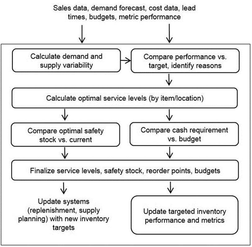
Figure 2-3. The inventory planning process
Once these uncertainty values have been updated, the next step is to calculate the optimal service level and the resulting safety stock requirements. The optimal service level is calculated based on several factors, including demand and supply variability, the projected demand, inventory holding costs, and shortage costs associated with inadequate inventory. These new targets are compared with the current values for safety stock (for material planning purposes) or reorder points (for replenishment). At this point, the workflow for accepting changes may differ by company depending on the number of items that need to be planned as well as item costs and margins. If there are several thousands of items, then a “control limits” approach can be used to automatically accept changes if they are below a threshold. However, if the differences exceed a certain threshold or if the cost of inventory is high, these changes can be manually reviewed. During manual review, the analyst needs to evaluate the reasons for the change, determine if any changes to the inputs (variability, lead times, and costs) need to be made, and redo the calculations, if necessary.
Once a list of changes has been created, the next step is to compare the implications of the change on cash requirements. Typically, inventory budgets are specified at a product line or facility level; therefore, the cash requirements across a set of items will need to be added and compared with the budget. If the requirements are higher, then the analyst has to determine, with help from finance, whether there is a reason to revise the budgets. However, if budget changes are not an option, then the analyst has to allocate the available cash to the different items. An example of a cash allocation procedure is provided later in this chapter.
The final step in the process is to export the data to other systems, including updated reorder points to replenishment systems, and updated safety stock targets to supply planning and materials requirements planning systems. Changes to these policies are also used to update targeted metrics—target turns and days of inventory, cash investment levels, and the updated gross margin return on inventory (GMROI).
The frequency with which the inventory planning process needs to be performed is determined by several factors, including the following:
· Updates to the demand forecast
· Updates to inventory budgets
· Addition of new products, customers, parts, and suppliers
· Addition of new distribution locations
Of these factors, only the first two are periodic in nature: demand planning is usually performed on a monthly basis, and budgeting is performed on a quarterly basis. Therefore, inventory planning is performed on a quarterly basis, with monthly reviews in case demand patterns have changed significantly. In addition, inventory planning will need to be performed on an as-needed basis as new products and facilities are added.
Measures of Inventory Performance
To determine how much inventory a company needs to maintain, it is first necessary to define a few metrics to represent goals. The most fundamental metric for maintaining inventory is customer service. If there is sufficient inventory, then the customer’s order is fulfilled in a timely manner and the customer is satisfied. Otherwise, the customer may have to wait, be offered a reduced price, or leave empty-handed and buy a competing product. A few common measures of inventory performance are briefly described below. (Chapter 7 describes at length the methods for evaluating and managing inventory performance.)
· Stockout service level. This is the probability of fulfilling all orders from inventory in a particular period. If an order is short-shipped even a single unit, then it is considered a stockout. This metric is useful in situations when a customer charges a penalty for receiving partially filled shipments. Another way to think about the stockout metric is the probability that stock will be depleted before the arrival of new supplies.
· Fill rate. This is the number of units fulfilled from inventory. This is less exacting than the stockout metric since credit is given for fulfilling a portion of the order. For example, if 100 units are ordered in a period that has only 95 units of inventory, then the fill rate is calculated as 95%. However, since not all 100 units were shipped from inventory, the stockout metric for this period is 0. The fill rate metric is useful when the penalty is best reflected by the number of units left unfulfilled, or when partial shipments are not penalized.
· Period fill rate. This is the number of units fulfilled from inventory and replenishments, as a proportion of the total units ordered in a time period. Since this measurement includes inventory that can be made available over a period of time, it is the least exacting of the three customer service measurements. This metric is useful when the turnaround time required by the customer allows for replenishments, after factoring the time taken to ship products to the customer.
· Days of inventory. The number of units or financial value of inventory, in isolation, can be misleading if demand changes significantly. A more revealing measure is days of inventory, measured as the number of days of sales that can be supported by the inventory. An alternative way to calculate this metric as the number of units of inventory divided by the average daily demand.
· Inventory turns. This is the number of times inventory is turned over in a year. When turns is calculated based on units of sales, then it is equal to the annual sales divided by average inventory over the year. Upon comparing this measurement with the days of inventory, it is easy to see that the two measurements share an inverse relationship and it is possible to derive one from the other. However, it is common to calculate turns based on the financial value of sales; the formula is the cost of goods sold divided by average inventory. This financial calculation can result in different values as compared to the units-based calculation due to cost variances over the year. Inventory turns is the most popular measure of inventory performance, and is also referred to as inventory turnover or stock turnover.
· GMROI. This is the income generated from every dollar spent on inventory, calculated as the annual profit divided by the average value of inventory over all the weeks of the year. Note that the GMROI aligns with return on assets for companies for which inventory is the primary operating asset, such as distributors and retailers.
Variability in the Supply Chain
Demand and supply variability are the primary factors driving the need for buffers in the supply chain (other factors include an increase in defective parts and lower-than-anticipated manufacturing yields). Demand uncertainty arises due to several factors—changing consumer preferences, economic conditions, environmental factors, new regulations, and competitive pressures, to name a few. Since it is impossible to eliminate these sources of variability, companies have attempted to reduce the impact by increasing the lead time that is available to satisfy demand (the order lead time). When the order lead time can be extended to the level that it is greater than the lead time required to procure raw material and manufacture product, then the company operates in a build-to-order (BTO) environment.
An example of a BTO environment is the custom furniture supply chain. Only after the order from the customer has been confirmed does the manufacturer order raw materials and produce the item. This results in delivery of product to the consumer four to five months after order placement. Due to this commitment provided by the customer, BTO models do not experience demand uncertainty. However, most companies do not have the luxury to dictate lead times. Retailers have to deal with zero order lead times since the product has to be available on the store shelves when the consumer walks into the store. Manufacturers usually have a one- to two-week order lead time to ship material after receiving the order from the retailer, and the manufacturer has no option but to manufacture products to a forecast. This situation is referred to as build-to-forecast (BTF) orbuild-to-stock (BTS). Short lead times are important in business-to-business situations as well, as underscored in this excerpt from an annual report of the Houston Wire & Cable Company:
Our cable management program is an inventory management system that pre-allocates specialty wire and cable for a customer’s specific project and includes a custom program designed to manage all of the wire and cable requirements for the project. The major benefits of our cable management program include guaranteed availability of materials, plus safety stock; immediate shipment of material upon field release; firm pricing and a dedicated project manager.
—Houston Wire & Cable Company, 2008 Annual Report
Chapter 3 provides additional examples and details regarding the impact of demand uncertainty on companies.
Another component of variability is related to supply, and this also increases the level of safety stock that is required. Supply-side variability is introduced due to several reasons, including variance in production activities at suppliers’ plants, an increase in the time taken to transport material due to load consolidation, an increase in the time taken to clear customs, as well as external factors such as weather. Examples of reasons contributing to a delayed shipment are shown in Figure 2-4.
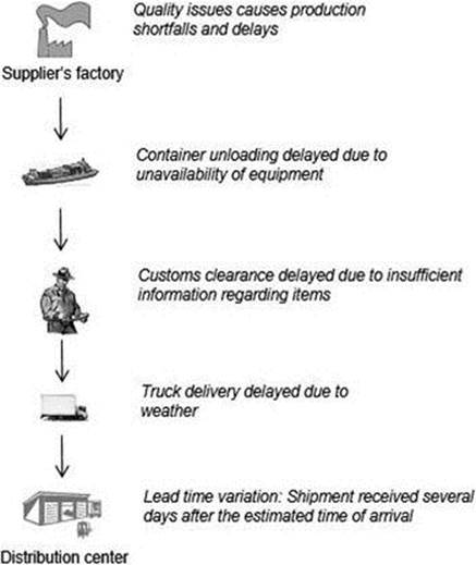
Figure 2-4. Examples of factors contributing to shipment delays
Supply lead time compounds the negative effect of variability in two ways. First, the forecasting horizon has to be increased to match this lead time, resulting in an associated increase in error. Second, inventory positions have to be committed to for the duration of the lead time, magnifying the impact of poor decisions.
An increase in lead times can raise the exposure due to unfavorable pricing of components for products that undergo high price erosion. Another by-product is an increase in work-in-process inventory (inventory that remains in various stages of manufacturing or transportation), which increases the cash-to-cash cycle time for suppliers. During tough economic conditions, tight cash flow situations can adversely affect the viability of small- and mid-sized companies.
Notwithstanding these drawbacks, lead times have steadily increased from the mid-1990s thanks largely to the promise of lower labor costs associated with outsourced, overseas manufacturing. The following excerpt from an annual report of Domino, a supplier of printing products, illustrates this extension and variance across products:
Our manufacturing operations benefited in 2010 from the restructuring and consolidation undertaken in the prior year. Cost efficiencies coupled with volume increases have enabled us to report an increase in gross margin rate to just below 50 per cent. This was achieved against a backdrop of increasing lead time in supply chains as global demand increased at a faster rate than component manufacturing capacity, and increased costs, in particular freight charges, as actions were taken to expedite parts supply to our factories. Whilst component availability was an issue in particular through the second quarter of the year, we were able to utilise buffer stocks to avoid any significant impact on supply to our customers. At year end the situation was largely back to normal, inventories have been replenished and lead times from our suppliers have returned to normal.
—Domino Printing Sciences plc, 2010 Annual Report
The excerpt emphasizes the importance of the close relationships with suppliers required to remain responsive in the face of increasing lead times. If such collaborative measures are not put in place, only a part of the anticipated benefit from outsourcing will be realized. Reasons that an increase in lead time results in lower flexibility and disruptions include the following:
· Reliance on partners for timely execution. The reliance on a different company for manufacturing can increase revenue risk when capacity is tight and the manufacturer is provided other more profitable opportunities to utilize capacity.
· Increased possibility of disruptive events. As the horizon for procurement and manufacturing increases, the number of disruptive events that can affect timely fulfillment also increase. Examples of these events include machine failures, industry-wide commodity shortages, and weather effects.
· More complex processes. Outsourced and off-shore manufacturing have introduced several additional steps in the delivery process, including ocean freight and customs clearance. These additional steps introduce variability due to dependence on other companies and governmental agencies, many more hand-offs, additional regulations, and additional paperwork requirements.
Supplier operations introduce variability related to production schedules, capacity shortfall, or rework due to poor quality resulting in delayed availability of goods. These sources of variability can be addressed by implementing appropriate processes for quality control and collaboration of relevant demand and capacity information.
In-bound transportation introduces variability related to missed shipment windows, unavailability of capacity, and extended wait times in order to consolidate loads. These issues can be partly or completely addressed by ensuring alignment between production and transportation schedules, and by communicating mid- and long-term shipment requirements to transportation providers.
Purchasing and information-sharing processes can introduce variability, either due to data errors while processing orders, delays in calculating purchasing requirements and communicating these orders to suppliers, or due to lumpy orders caused by consolidation and pricing concerns. Data errors can be reduced by the use of systems to limit manual inputs. Furthermore, systems can help with timely processing of purchases and communication of orders. Finally, lumpy demand can be eliminated by negotiating price agreements based on quarterly or annual purchasing amounts (as opposed to each individual shipments), or by the use of low-cost transportation options for small shipments.
Finally, supply variability can be caused by external factors such as inclement weather, heavy seaport traffic and congestion, or customs delays. While little can be done to reduce the variability associated with these factors, good planning can help mitigate the effects. Table 2-3 lists some examples of variability and management aids to reduce or deal with each.
Table 2-3. A Few Methods to Address Supply Variability
|
Category |
Source of Variability |
Management Aids |
|
Supplier operations |
Capacity shortages. |
Collaboration related to capacity, production schedules, and purchase orders. |
|
Transportation |
Unavailability of transportation equipment. |
Forecast collaboration. |
|
Information sharing |
Delay in communication of orders to suppliers. |
Rigorous replenishment process to release purchase orders in a timely manner. |
|
External factors |
Weather. |
Use of safety stock. |
Safety Stock (Buffer Inventory)
Since a majority of businesses operate in an environment where material is produced ahead of firm customer orders (build-to-forecast), there is a widespread need to hold buffer inventory. This buffer inventory is required to fulfill higher-than-expected demand as well as a cushion against delayed arrival of raw materials. Supply chain professionals have long dealt with buffer inventory, and the most common methods employed to determine these levels are the service level model and the newsvendor model. The service level method determines inventory levels based on the probability of meeting demand. This determination is based solely on the uncertainty that is inherent in demand and not on any financial consideration. On the other hand, the newsvendor model determines optimal inventory levels according to a trade-off between the profit obtained from holding inventory against an estimate of the cost of holding inventory. Though the newsvendor model is attractive due to its simplicity, it makes several assumptions that make it applicable only to products with short lifecycles (for example, newspapers—hence the name—or groceries). It is therefore necessary to utilize a different model for products that do not become obsolete in a short period of time. Such a model, called the incremental margin model, is introduced toward the end of the section.
The Service Level Method
The service level method estimates the safety inventory in consideration of the uncertainty of demand over the lead time for supply (Figure 2-5). Demand variability or uncertainty is commonly specified using the variability in demand (when replenishment models such as reorder points are used for maintaining inventory levels), or by the standard deviation of the forecast error (when forecasts and material requirements plans are used to maintain inventory levels). The entire value of uncertainty is determined by multiplying the variance in forecast error with the supply lead time since an inventory position needs to be taken for the entire duration of the lead time. The model also requires the estimation of a service level factor (k), which represents a measure of the probability of meeting demand directly from on-hand inventory, referred to as the service level. Thestockout service level is defined as the probability that demand can be met from on-hand inventory. The value of k depends on the nature of probability distribution that best describes the demand signal. It is common to use the normal probability distribution unless the analyst can determine a more appropriate distribution. Figure 2-5 lists values of k for various service level values. Higher values of k result in higher inventories and service levels.
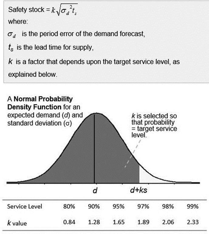
Figure 2-5. Illustration of the service level method for determining safety stock
EXAMPLE 2-1: APPLYING THE SERVICE LEVEL METHOD
Demand (actual sales) and forecast data for a consumer good are shown in Figure 2-6 for eight months of history. Since the lead time for supply is two months, orders are based on the two-month prior forecast. Forecast error is calculated as the difference between actual sales and the two-month prior forecast, and the root mean square error (RMSE) is calculated to be 2,123 units (i.e., 19% of average monthly sales), as shown in Figure 2-6.
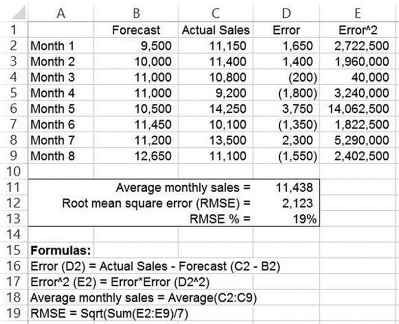
Figure 2-6. Procedure for determining forecast errors
In the spreadsheet, the RMSE has been calculated according to Equation 2-1.
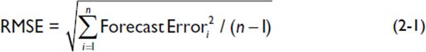
where n is the number of observations. If the company desires a service level of 95%, the equivalent value of k is 1.65 (from Figure 2-5). From the same figure, the safety stock is calculated as
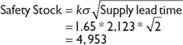
Therefore, the company should hold 4,953 units (approximately 12 days of inventory, based on average monthly demand) in order to provide the desired service level. If a service level of 99% is desired, then the calculation would result in a safety stock of 6,994 units (approximately 18 days of inventory).
The popularity of the normal distribution for representing the probability of forecast error is not arbitrary. Under certain situations, statistical estimates converge to a normal distribution, as outlined by the central limit theorem.1
While it is important to select the appropriate probability function, in reality no single function can accurately represent demand. Therefore, a certain amount of error in inventory estimates cannot be avoided, and it is necessary to monitor performance and make adjustments when needed. Such a review procedure is described in Chapter 5.
In practice, the standard deviation of demand (demand variability) has often been used instead of forecast error in the equation. This assumption is acceptable when demand is steady, uniform, and without seasonal effects. However, if seasonality exists and the forecasting method accounts for these effects, the use of standard deviation of demand can result in excessively high-inventory requirements since demand can fluctuate more than the forecast error, as illustrated in Figure 2-7. Therefore, the use of standard deviation of demand for calculating inventory requirements is not recommended.
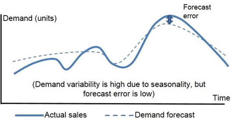
Figure 2-7. Potential issues in the use of standard deviation of demand vs. standard deviation of forecast error for calculating safety stocks
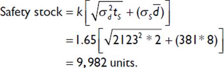
In many practical situations, safety stock is required to cover demand uncertainty as well as supply variability. Supply variability refers to the difference between the expected and actual delivery time for raw materials. Since supply variability introduces additional uncertainty, additional inventory is required to provide the same service level. This additional inventory can be calculated by modifying the equation in Figure 2-5 to include a supply variance term, as shown in Equation 2-2.
![]()
where the first term under the square root symbol is the same as in Figure 2-5, and the second term represents the additional inventory requirement due to supply variability. represents average demand and σS represents the standard deviation of the differences between the actual and expected supply lead times.
The equation assumes that the variabilities in demand and supply are not related (i.e., they are independent of each other)—for this assumption allows a combined variance to be calculated as the sum of the two individual variances. But if the uncertainty in demand is correlated with variability in supply, this calculation is not valid. Instead, the safety stock has to be calculated separately for the two terms, as shown in Equation 2-3 for the perfectly correlated case.
![]()
The difference between Equation 2-2 and Equation 2-3 is that in the latter the variances are not combined and safety stock is computed separately for each. Note that the correlated case will always result in a higher inventory level than the independent case. When demand and supply uncertainties are not perfectly correlated, the required safety stock will be in between these two estimates. For formal treatments of covariance and correlation, consult any standard statistics textbook.2
It is desirable to use the safety stock calculation for the independent case since it results in lower inventories. However, independence requires that production capacity (at the company and key suppliers’ manufacturing plants) be far greater than any unanticipated increase or decrease in demand. This condition is often not true for dedicated production lines and manufacture of custom parts since production capacity is usually set based on an expected value of demand. In such cases, higher-than-expected demand will result in tight capacity and a corresponding increase in production lead time. Therefore, unless it is possible to determine that supplies for all assemblies and parts for a product are independent of demand, it is recommended that the second method (covariance) be used for calculating safety stock. Similarly, transportation lead time variances may need to be considered as correlated if the company expects a significant company-wide increase in demand or the entire industry is experiencing an increase; in such cases, the transportation providers may face a similar shortage of transportation capacity, and lead times will increase as it takes longer to find free ocean containers or trucks.
EXAMPLE 2-2: APPLYING THE SERVICE LEVEL METHOD FOR DEMAND UNCERTAINTY AND SUPPLY VARIABILITY
For the data given in Example 2-1, the time taken to receive goods has been noted to differ from the expected lead time of one month. Data is collected for eight months of history and is shown in Figure 2-8. The average lead time is calculated to be 37 days and supply variability (as measured by the root mean square error, where error is the difference between actual and expected lead time) is calculated to be 8 days. The spreadsheet formulas for the calculation are shown in the respective cells.
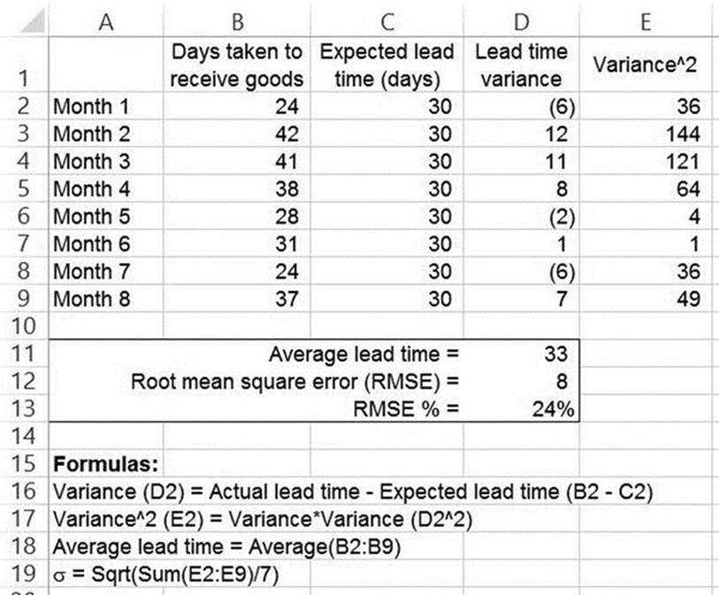
Figure 2-8. Procedure for determining supply lead time variance
With this information, safety stock requirements can be calculated based on demand and supply variability. Since the supply lead time variability is in days, the daily average demand needs to be used for units to be consistent. The calculation is
Average daily demand = 11,438 / 30 = 381 units.
If demand and supply variability are assumed to be independent, then the calculation for a 95% service level is
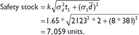
Therefore, safety stock levels have increased from 4,953 (Example 2-1) to 7,059 units due to supply variability. This translates to an additional 6 days of inventory, resulting in a total of 18 days. If the analyst perceives that the supplier’s production capacity is tight and that any increase in demand will be accompanied by delays in supplies, then perfect correlation results in the following calculation of safety stock by Equation 2-3:
The results reveal that covariance has resulted in an additional 2,923 units, or 8 days of inventory, for a total of 26 days. Depending on the cash positions of the company, the analyst can select a safety stock level between the two values—18 days if the available budgets are tight and 26 days if customer service and material availability are the priority.
An advantage of separating inventory requirements for demand and supply variability is that the magnitude and improvement areas are apparent. For example, if most of the safety stock requirement is to cover for uncertainty in demand, then the areas requiring improvement are forecasting and collaboration with channel partners. On the other hand, if supply variability has a large impact, then areas to focus on include capacity alignment and collaboration with key suppliers.
In conclusion, the service level method is simple to use and provides an important connection between inventory level and customer service. On the other hand, this method suffers from the following limitations:
· No guidance is provided regarding the optimal service level for an item. For example, is a 95% service level excessively high? Intuitively, it would appear that a higher service level should be provided for a high margin item, as compared to an item with a lower margin. However, the service level method provides no guidance regarding how service levels should be tailored by item.
· No guidance is provided regarding the price required to provide a service level to a customer, because costs, margins, and price are not included in the formulation.
Addressing these questions requires that the financial aspects related to inventory be included in the model. A simple method for performing this analysis is the newsvendor model, described next.
The Newsvendor Model
The newsvendor model can be readily understood from the following statement of the problem. Consider a newsvendor who needs to determine the quantity of newspapers that needs to be purchased for each day. If demand is greater than the purchased quantity, then the benefit (margin) from that additional demand is lost. On the other hand, if the purchased quantity is greater than demand, then the leftover newspapers are not sold and are disposed of the following day as scrap. Given that the demand on any given day is not specified (it varies randomly), how should the optimal inventory be determined?
The model is based on balancing two costs: the shortage cost and obsolescence cost (also referred to as the scrap cost), defined as follows:
· The shortage cost (cS) is the penalty for not meeting demand. This cost depends on the sales model of the company and, in business-to-business cases, on customer obligations and contracts. For example, the shortage cost for a retailer is the margin that is lost due to inventory not being available. For a food manufacturer shipping goods to a retailer, the shortage cost could be a financial penalty for each order that is not shipped in its entirety (ship-complete). In addition to penalties, shortage costs can also include expedite costs related to rush transportation, such as air shipments vs. ocean, or less-than-truckload shipments vs. full truckloads.
· The obsolescence cost (co) is the penalty due to inventory that is not sold. It is calculated as the difference between the cost of procuring or producing the item and the salvage price that can be obtained for the leftover inventory (i.e., unit cost minus salvage price). Note that the newsvendor model is a single-period model, and it requires that the salvage price be lower than the unit cost. If this is not the case, a multi-period model needs to be utilized. (One such model is developed in the following section.)
The important aspect of the newsvendor model is that it explicitly considers demand to be a random variable, characterized by an expected value and a forecast error. The derivation of the model is shown in Figure 2-9. In the figure, the first equation lists the profit function as the margin obtained from sales minus two cost terms. The first term is due to holding excess inventory, calculated as the unit obsolescence cost multiplied by excess inventory. The second term is due to inventory shortage, calculated as the unit shortage cost multiplied by the number of units of demand that cannot be met from on-hand inventory. Because demand is random, it is necessary to calculate an expected value of the cost incurred by assuming a particular probability function for demand. In the derivation shown, a normal probability function has been used to specify demand, which uses a bell curve to determine the probability that demand will be greater or less than the expected value. With this assumption, the optimal level of supply is determined by differentiating the profit function with respect to the level of supply s, and setting that expression to zero. This results in the following formula for determining the optimal service level and supply:
![]()
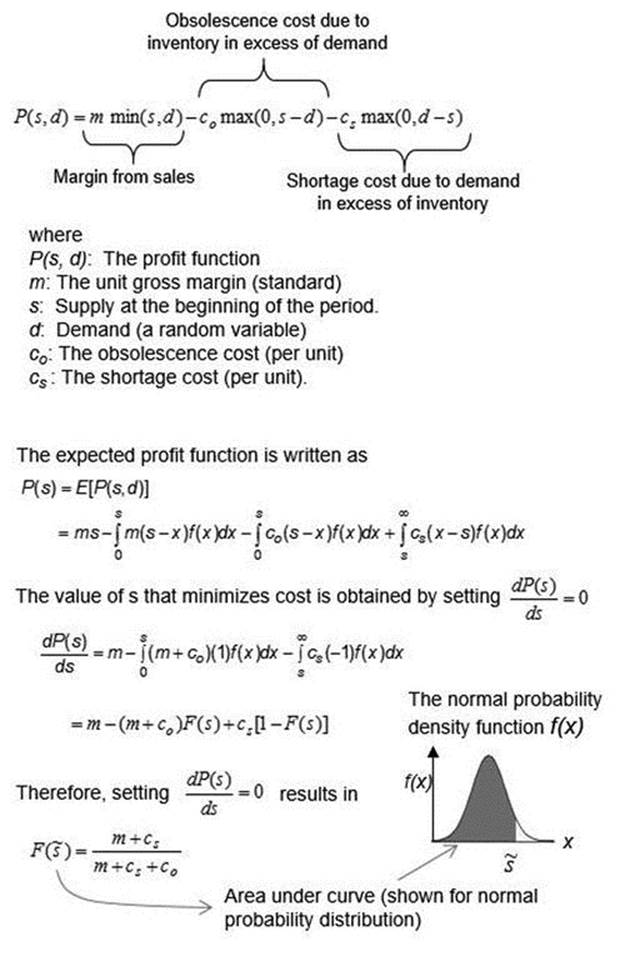
Figure 2-9. The newsvendor model derivation
where ![]() is the optimal supply. The standard deviation σ represents the combined variability due to demand and supply, calculated according to Equation 2-2. The term
is the optimal supply. The standard deviation σ represents the combined variability due to demand and supply, calculated according to Equation 2-2. The term ![]() is the cumulative probability function, calculated in Microsoft Excel by the formula NORMDIST
is the cumulative probability function, calculated in Microsoft Excel by the formula NORMDIST ![]() . It represents the optimal service level because it captures the probability of meeting demand. The cost ratio in Equation 2-4 is sometimes referred to as the critical fractile.
. It represents the optimal service level because it captures the probability of meeting demand. The cost ratio in Equation 2-4 is sometimes referred to as the critical fractile.
The newsvendor model is useful for estimating supply targets over a single month, quarter, or other period of a supply contract, as long as price and costs are constant throughout the period. Another assumption made by the model is that the product needs to be disposed at a scrap value at the end of the period. While these assumptions do limit the number of situations that the model can be applied to, the fundamental insights provided by the model are still very useful. Therefore, this model will be studied in depth in the following pages preliminary to the development of a model that is applicable to a broader variety of situations.
Newsvendor Model Applied to a Retail Situation
The situation considered in Example 2-3 is a perishable product stocked on the retail shelf, such that any demand that is in excess of the inventory on the retail shelf is lost. Because retail products are replenished on a frequent basis (typically one to two times per week), it is possible to apply the newsvendor model to products for which the lifespan is aligned with the replenishment schedule.
EXAMPLE 2-3: APPLICATION OF THE NEWSVENDOR MODEL TO A PERISHABLE GROCERY PRODUCT
An expected weekly demand for a grocery item is 10,000 lbs, with a forecast error of 20%. Inventory is replenished on a weekly basis. The item is purchased for $1.50 per pound and sold for $2.50 per pound. The product lifespan is approximately one week, and any leftover inventory is thrown away.
Determining the Optimal Inventory Level
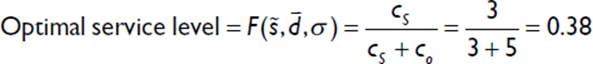
Because leftover inventory has no value, the obsolescence cost is the purchase price, $1.50 per pound. The company incurs no penalty for insufficient inventory. Therefore, the optimal service level is calculated from Equation 2-3 as
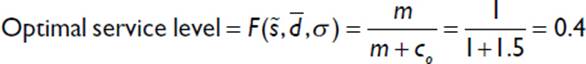
The model dictates an optimal service level of 40%. For expected demand of 10,000 lbs and forecast error of 2,000 lbs (= 20%*10,000), the optimal order quantity can be determined from the following spreadsheet function:
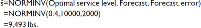
Therefore, the model dictates that the company should order 9,493 lbs every week. Note that this quantity is less than the expected demand, due to the high obsolescence costs.
It is possible to build upon the model and compute other useful measures.
where the Microsoft Excel functions for the distribution terms are
![]()
The expected sales is calculated as
![]()
The expected fill rate is calculated as
![]()
where the expected demand is and expected sales is derived from Equation 2-6. The expected leftover inventory is calculated as
![]()
Expected values for costs and profits can now be calculated. The expected holding cost is the unit holding cost multiplied by the leftover inventory.
![]()
The expected shortage cost is the unit shortage cost multiplied by lost sales.
![]()
The expected profit is the margin from expected sales minus the costs incurred due to obsolescence and shortage:
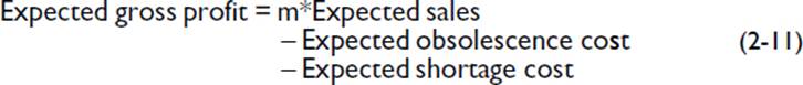
where m is the target unit margin (selling price minus buying price). Finally, unit margins are calculated as
![]()
The unit margin is a useful measurement for comparing against target margins and providing guidance regarding prices.
Continuing the retail example, the following are computed:
Optimal service level = 0.40.
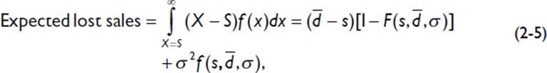
Optimal supply level = 9,493 lbs.
Expected lost sales = 1,076 lbs (from Eq. 2-5).
Expected sales = (10,000 – 1,076) = 8,923 lbs (from Eq. 2-6).
Expected fill rate = 8,923/10,000 = 89% (from Eq. 2-7).
Expected leftover inventory = 570 lbs (from Eq. 2-8).
Expected obsolescence cost = $855 (from Eq. 2-9).
Expected shortage cost = $0 (from Eq. 2-10).
Expected revenue = expected sales * price = 8,923 * 2.50 = $22,307.50.
Expected gross profit = $8,068 (from Eq. 2-11).
Expected unit margin = $0.85 per lb. (from Eq. 2-12).
Therefore, the gross margin that the company can expect is $0.15 less than the targeted margin of $1 per lb. If the company wishes to achieve a margin of $1, the price would need to be changed to $2.66 per lb.
Consider another situation: The company’s management is not comfortable with such a low service level because of stockout concerns and concern that customers may be driven to other stores with better inventory positions. Instead, a target service level of 90% is desired. This service level results in the following:
Service level target = 0.90.
Required supply level = NORMINV(.90, 10,000, 2,000) = 12,563 lbs.
Expected lost sales = 95 lbs.
Expected sales = 9,905 lbs.
Expected fill rate = 9,905/10,000 = 99%.
Expected leftover inventory = 2,658 lbs.
Expected obsolescence cost = $3,986.
Expected shortage cost = $0.
Expected gross profit = $5,919.
Expected gross margin per unit = $0.47 per lb.
Therefore, the higher service level has resulted in significant margin erosion due to the increase in scrap inventory. If the company wishes to retain its margin of $1 per lb, then the price would need to be increased to $3.17 per lb.
The model can be used for several other analyses, such as analyzing the impact of variability on margins. Figure 2-10 illustrates how an increase in variability results in margin erosion. By quantifying the impact, management can decide whether to invest in systems or new procedures to reduce forecast error.
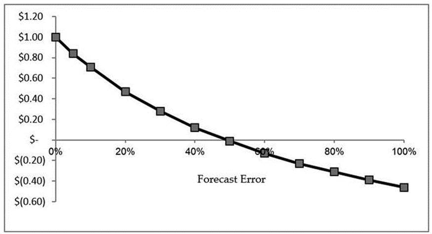
Figure 2-10. Impact of variability on unit margins
The example in Figure 2-10 illustrates the usefulness of the newsvendor model in considering variability and costs in order to provide guidance regarding supplies, service levels, and prices for a given retail situations.
Newsvendor Model Applied to a Strategic Buy Situation
In this section, the newsvendor model is applied to a business-to-business situation involving a strategic purchase. Unlike the retail situation, the company can meet unmet demand by increasing production but incurs thereby a shortage penalty.
A company sells its goods through retail channels and needs to place a production order with its contract manufacturer for purchasing a certain quantity of the product line for an entire season. While the company can estimate the expected demand, it is subject to significant error since the order has to be placed well in advance of sales. If demand is greater than the quantity ordered, then the company is allowed to order additional volume, but the contract manufacturer will tack on an additional cost to cover its expenses related to additional raw material purchases or due to overtime labor. Conversely, if demand is less than quantity ordered, then the company will be left with unsold inventory at the end of the season; this inventory can be disposed, but at a steeply discounted rate.
The company needs to decide what order quantity it needs to place with the contract manufacturer.
The newsvendor model can be used to answer this question. The model requires the following quantities to be determined:
· The expected demand (i.e., forecast) for the entire season. This quantity can be determined based on sales of the same or similar products for the prior year, adjusted for market conditions.
· The error associated with the forecast so determined. This quantity can be calculated by comparing the forecasts for prior seasons compared to actual sales.
· The obsolescence cost for excess inventory. Since leftover inventory at the end of the season has to be disposed at a lower price, the obsolescence cost is the purchase cost less salvage value.
· The shortage cost for unmet demand. This is the additional cost charged by the contract manufacturer for units in excess of the contracted quantity.
Once these quantities have been determined, the profit equation for this flexible production policy can be written as
![]()
Equation 2-13 is developed for the case when sales in excess of supply are not lost since the option of increasing production is available (the model assumes that sufficient lead times exist to increase production and satisfy retail orders). Therefore, this profit equation is different from Equation 2-9, which is developed for the case when sales in excess of supply are lost. Following the procedure in Equation 2-9 for maximizing profits, the optimal service level is calculated as
![]()
EXAMPLE 2-4: APPLICATION OF THE NEWSVENDOR MODEL TO DETERMINE SEASONAL PURCHASE QUANTITIES
An apparel design company has created a line of products for the winter season spanning November through March. The company uses a contract manufacturer for production, and is required to place the order by June in order to receive shipments by November. The company estimates the demand for the product line to be 150,000 units, and the forecast error (RMSE) is estimated to be 20%. The purchase cost is $15 per piece. The company desires a $10 margin and set the price at $25 accordingly. Any unsold inventory can be disposed at $10 per piece. Finally, any production in addition to the contracted amount will be satisfied with an incremental cost of $3 per piece to cover any additional costs incurred by the manufacturer.
Determining the Optimal Service Level and Order Quantity
The shortage cost is $3 per piece, while the obsolescence cost is $5 (= purchase cost – salvage price = $15 - $10). From Eq. 2-14, the optimal service level is calculated as
The model dictates an optimal service level of 38%. For expected demand of 150,000 units and forecast error of 30,000 (= 20%*150,000), the optimal order quantity can be determined from the following spreadsheet function:
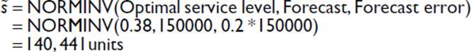
Therefore, the model dictates that the company should place an order for 140,441 units with the contract manufacturer. If demand is higher than this level, then additional orders can be placed with the contract manufacturer.
As with the previous case, additional measurements can be generated using the model. This situation differs from the previously described retail situation in that demand in excess of inventory is not lost, because the apparel company has the option of increasing production, such that
![]()
However, there is a possibility that production will need to be increased, which is estimated as
Because there are no lost sales, the expected sales is simply the expected demand,
![]()
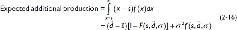
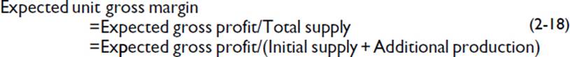
The expected leftover inventory, obsolescence cost, shortage costs, and gross profit are calculated as in the previous case (Equations 2-8 through 2-11). The unit margin is calculated according to Equation 2-18:
Continuing Example 2-4, the following fields are computed:
Target service level: 38%.
Expected additional production = 17,350 (from Eq. 2-16).
Expected leftover inventory = 140,441 – 150,000 + 17,350 = 7,791.
Expected obsolescence cost = $5 * 7,791 = $38,956.
Expected shortage cost = $3 * 17,350 = $52,051.
Expected profit = $10*150,000 - $38,956 - $52,051 = $1,408,993.
Expected gross margin per unit = $1,408,993 / (140,441 + 17,350) = $8.93.
Therefore, the model indicates that the margin that can be expected is less than the anticipated margin of $10, and price would have to be increased by approximately $1.07 to compensate for obsolescence and shortage costs that may be incurred.
The newsvendor model also provides insight into the impact of supply uncertainty. Due to supply variability, a greater level of supply is required to provide the same service level. However, when supply is in excess of the optimal value, the expected margin will decrease, per the newsvendor model. This calculation is shown in Figure 2-11 with the negative impact of supply variability being dictated by the magnitude of obsolescence cost.
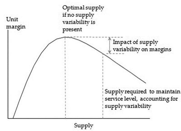
Figure 2-11. Impact of supply variability on margins
The examples above illustrate the usefulness of the newsvendor model and how it can be used to provide guidance regarding prices, profits, and policies. There is, however, a significant drawback to this model: it is a single-period model, with any leftover inventory at the end of the period being disposed at a scrap value. (The period for inventory calculation purposes is the replenishment frequency, which can range from daily when suppliers are local to monthly for overseas shipments.) Because most products have lifecycles that can last several months or even years, the single-period assumption is a severe limitation since these products can continue to be sold beyond a single replenishment period. Also, due to this single-period applicability, situations involving variations in price, costs, and demand over time cannot be accommodated. The first requirement of a generalized inventory model is the ability to accommodate multiple time-periods. The incremental margin model is one such method.
The Incremental Margin Model
The incremental margin model extends the newsvendor model to multiple periods. In addition to the costs included in the newsvendor model, a multi-period inventory planning model needs to include another penalty—the holding cost. This is the penalty for holding inventory for a certain period of time and includes the cost of storage, insurance, and spoilage. Costs that are already present in the cost-of-goods calculation (for raw materials, production, handling, and transportation) should not be included. Only those costs that are incurred due to inventory being held for a certain period of time should be included.
A multi-period inventory planning model needs to provide the following capabilities:
· Allow for inventory that is left over at the end of one period to be sold in the following period.
· Allow for the expected demand and forecast error to vary across periods.
· Allow for the shortage cost, holding cost, and price to vary across periods.
· Allow the product to be sold at a salvage value at the end of any period.
The multi-period model developed in this section is referred to as the incremental margin model, since costs and margins are incrementally calculated for each period. The gross profit from s units of supply is calculated by subtracting shortage, holding, and obsolescence costs from the total margin. For the situation in which prices and material costs are uniform across the periods, this is calculated according to:
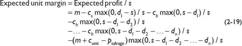
where n represents the number of periods corresponding to the shelf-life of the item. Each of the terms in the equation is explained as follows:
· The first cost term is the shortage cost, as explained for the newsvendor model. It represents the penalty incurred in case shipments are not made in a timely manner, or the cost of expediting to meet demand on time.
· The subsequent cost terms are the holding costs incurred by holding inventory for the first and subsequent periods. Note that this holding cost is a period cost and includes the cost of capital. This cost is different from the obsolescence cost term in the newsvendor model.
· The final cost term is the loss due to obsolescence for the case when the product has a shelf-life of n periods. Since the first term includes margin from the entire s units of supply, the margin lost due to obsolete inventory needs to be deducted. Also, if obsolete inventory can be disposed for a price (the salvage price), then the resulting return is calculated by multiplying the salvage benefit with the leftover inventory. The salvage benefit is calculated as the difference between the salvage price and the unit cost.
The expected profit per period is calculated according to Equation 2-20:
![]()
where the expected unit margin is calculated by Equation 2-19. The expected sales depends on the sales situation and demand retention policy adopted by the company. If unmet sales are lost (as in retail situations or when a company chooses not to expedite or offer incentives to the customer to retain demand), then the expected sales are given by Equation 2-6. On the other hand, if unmet demand can be retained or backlogged, then lost sales is zero and the expected sales equals the expected demand.
Appendix B presents a detailed development of the incremental margin model and the methods needed to perform the computations using spreadsheet functions. An application of the model is given in Example 2-5.
EXAMPLE 2-5: APPLYING THE INCREMENTAL MARGIN MODEL
Consider the grocery item in Example 2-3 with a shelf-life of 2 weeks. After 2 weeks, the product has no value and is disposed. Demand, costs, and price remain uniform across the 2 weeks. The holding cost is estimated to be $0.01 per lb per week and includes the cost of capital and other inventory-related costs.
Determining the Optimal Inventory Level
The optimal supply is determined by plugging in different values for s into Equation 2-19 until the gross margin is maximized to arrive at value of 14,100 lbs. Recall that the optimal supply in Example 2-3 for the 1 week shelf-life was 9,493 lbs. Therefore, increasing the shelf-life from 1 to 2 weeks results in a significant increase in the optimal order quantity. The following fields can be computed:
Optimal supply = 14,300 lbs.
Service level target = 98%.
Expected lost sales = 15 lbs (from Eq. 2-5).
Expected sales = (10,000 – 15) = 9,983 lbs (from Eq. 2-6).
Expected fill rate = 9,983/10,000 = 99.9% (from Eq. 2-7).
Expected leftover inventory = 4,155 lbs (from Eq. 2-8).
Expected unit margin = $0.993 per lb. (from Eq. 2-19).
Expected gross profit = $9,912 (from Eq. 2-20).
The expected gross margin for various supply levels is shown in Table 2-4 and Figure 2-12. High values of lost sales cause the steep decrease in margins toward the left, while the gradual decrease in margins after 13,800 units is due to a comparably lower penalty associated with holding costs. After approximately 15,000 units, margins decrease rapidly due to the increased probability of scrap inventory.
Table 2-4. Impact of Shelf Life on Expected Margins
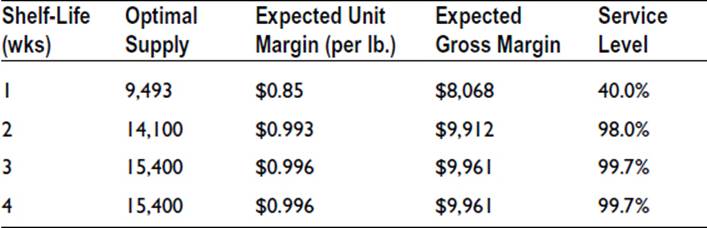
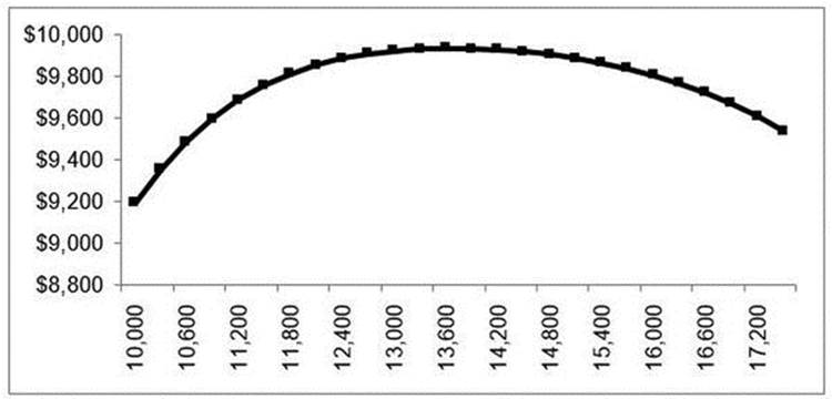
Figure 2-12. Using the incremental margin model to calculate expected margins
Recall that the expected unit margin for 1 week of shelf-life (Example 2-3) was $0.85/lb. The increase in shelf-life from 1 to 2 weeks has increased the expected margin significantly due to the reduced penalty from scrap. The impact of shelf-life on optimal supplies and margins is shown in Table 2-4.
As expected, the increase to 3 weeks has a large impact on optimal supplies. However, the additional increase to 4 weeks has minimal impact since the probability of obsolete inventory is minimal (due to low demand variability).
This multi-period inventory model can be used to understand the impact of shelf-life on optimal supplies and margins. The flexibility provided to model lifecycle demand and end-of-life scrap loss is very useful for industries such as grocery, pharmaceuticals, and electronics. Consider the following excerpt from an annual report of Regeneron, a biotechnology company:
Cost of goods sold increased to $118.0 million in 2013 from $83.9 million in 2012 due primarily to increased sales of EYLEA. In addition, in 2013 and 2012 , cost of goods sold included inventory write-downs and reserves totaling $9.1 million and $17.0 million, respectively. We record a charge to cost of goods sold to write down our inventory to its estimated realizable value if certain batches or units of product do not meet quality specifications or are expected to expire prior to sale.
—2014 Annual Report, Regeneron
Increasingly, other industries are being similarly impacted, partly due to fast-changing customer preferences and the increasing presence of embedded electronics in consumer products.
In conclusion, the incremental margin model provides an important extension of the newsvendor model to multiple periods and time-varying prices and demand. The flexibility of this model allows for several business situations to be analyzed, such as price rebates, end-of-life ordering, and cash budgeting. The remaining sections of the chapter cover such topics.
Batch Inventory
Batching refers to the production, purchasing, or transportation of material in certain lot sizes, potentially resulting in inventory in excess of the target. Batching is performed primarily to reduce costs—to take advantage of quantity discounts offered by suppliers, minimizing unit transportation costs by shipping full truck or container loads, and minimizing setup-related costs in manufacturing. The most common method for determining batch sizes is the economic order quantity (EOQ) model, which considers the following costs:
· Manufacturing setup, transportation, or purchase-ordering costs, calculated as a fixed cost incurred for each order.
· Holding cost, including the cost of money, warehousing, and other inventory related costs. This cost is calculated based on the average inventory levels, calculated as Order Quantity/2. (See Chapter 4 for a detailed description of holding costs.)
The derivation of the model is shown in Figure 2-13. Example 2-6 illustrates the use of the EOQ model for a single product.
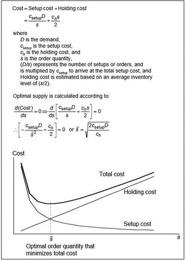
Figure 2-13. The economic order quantity (EOQ) model
EXAMPLE 2-6: APPLYING THE EOQ MODEL TO A PRODUCTION SITUATION
A food item manufacturer estimates that the time taken to prepare the production line for a particular item is 30 minutes. The daily output of the line (based on an eight-hour shift) is $500,000. The monthly demand for the item is 250,000 units, and the holding cost is estimated to be $0.25 per unit per month. The manufacturer wishes to determine the economic quantity for production.
Calculating the Economic Production Batch Size
The average output for 30 minutes is calculated as ($500,000/16) = $31,250. Since this output is lost while preparing the production line, this is set equal to the setup cost. Applying the equation shown in Figure 2-13 yields the result,
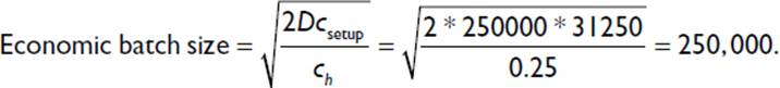
Therefore, the economic production quantity is equal to the monthly demand. The number of setups, calculated as (Demand/EOQ), is 1. Therefore, the EOQ model dictates that production needs to occur only once at the beginning of the month, and that the inventory be stocked for that entire duration.
In addition to the constant demand assumption, the EOQ model assumes that demand is known with certainty. Since most companies deal with uncertain demand, the guidance provided by the EOQ model will be suboptimal in the form of excess inventory and holding costs or insufficient inventory and shortage costs. Therefore, in most situations, the EOQ model needs to be used in conjunction with the safety stock models discussed in the previous section: the service level, newsvendor, and incremental margin models. The safety stock models need to be used first to determine the optimal supply quantity, which becomes the input for the EOQ model (as the demand) and is substituted in the equation to calculate batch or lot sizes.
Inventory Budgeting
Since inventory of raw materials and finished goods may be needed several weeks or even months in advance of sales, companies need to invest cash in order to purchase and manufacture inventory. This invested cash is eventually recovered when the product is sold at a profit. The use of cash for purchasing and storing inventory is one of the most important business decisions for a company since it has an impact on margins, cash flow, and viability. Consider the following excerpt from an annual report of STEC, Inc., an electronics manufacturer, on the impact of inventory investment on profits:
Interest income and other is comprised primarily of interest income from our cash, cash equivalents and marketable securities. Interest income and other decreased from $3.8 million in 2007 to $1.3 million in 2008 as a result of a lower average cash balance in 2008 compared to 2007 and a reduction in interest rates in 2008. The reduction in the average cash balance was due primarily to use of cash for inventory purchases related to new SSD product sales in 2008.
—2008 Annual Report, STEC, Inc.
The need to tie up cash for inventory is unavoidable for most companies. However, when inventory does not move quickly, this cash is tied up for an extended period of time and poses two issues. First, the interest generated from the cash value is lost for the entire duration. Second, generally accepted accounting principles require that inventory that has not moved for a certain period of time (say, six months) be declared obsolete, in which case the entire cash investment is lost.
There are two aspects regarding inventory budgeting. The first is to determine the required budget, based on determining the required cash followed by a return-on-inventory analysis. The second is to manage to these budgets and allocate cash when variances occur. The first aspect is discussed here; the second aspect is further described in Chapter 5.
Inventory budgets are usually specified for an item group or all items in a facility. The rigorous procedure outlined here is recommended, along with steps to rationalize the product portfolio to weed out underperforming products. The steps for determining inventory budgets are as follows:
Step 1: Plot the supply network for the products to understand lead times and the value-add at each step.
Step 2: Calculate the inventory investment required for each stage of the supply chain. Sum across all products to obtain the required inventory investment.
Step 3: Calculate inventory metrics—days of inventory, turns, and GMROI for future budget adjustments and allocations.
These steps are illustrated in Example 2-7.
EXAMPLE 2-7: DETERMINING INVENTORY BUDGETS FOR AN ELECTRONICS MANUFACTURER
ABC Co. has budgeted $360,000 for its product line inventory. The anticipated demand is 10,000 units per month, the product is priced at an average of $20 per unit, and the unit cost is $12 per unit. Is this budget for 3 months of inventory sufficient for supporting operations and providing the targeted customer service?
Step 1: Plot the Supply Network
A sample depiction of the supply network is shown in Figure 2-14. For each stage in the supply chain, the following information is captured: inventory ownership, cost of inventory or value-add, lead times, and billing terms. In this example, ABC Co. purchases raw materials directly from the supplier and stocks the raw material at the contract manufacturer’s facility. The cost of production is primarily labor. ABC Co. is responsible for the shipping process and receives materials into inventory at its distribution centers.
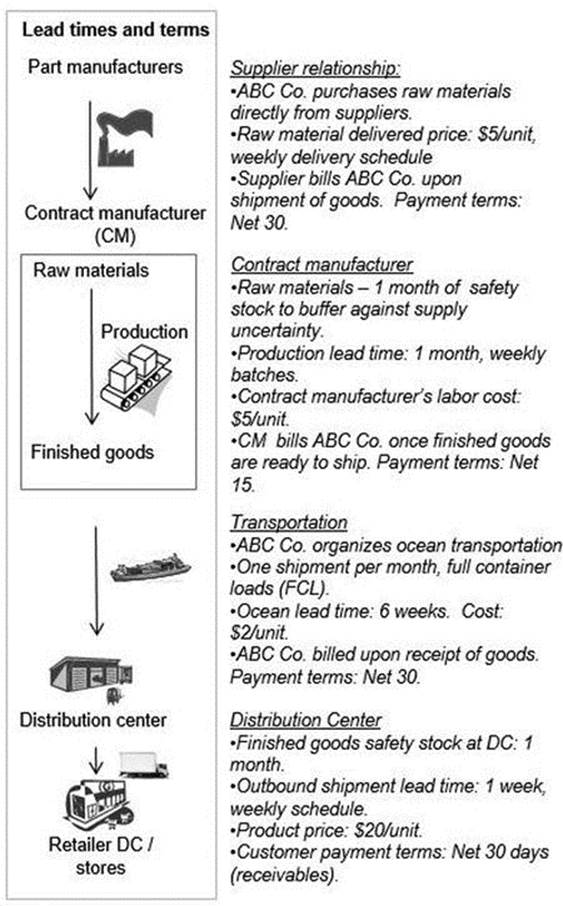
Figure 2-14. Sample lead times and contractual terms for Example 2-7
Step 2: Calculate Inventory Investment Required for Each Stage of Supply Chain
The investment is calculated as a combination of cycle stock, safety stock, and work-in-process for raw materials, intermediate (or assemblies), and finished goods. Each of the stages is described below.
Raw Materials at the Contract Manufacturer
Since ABC Co. purchases raw materials directly from the supplier and takes ownership of the inventory, the inventory investment is calculated as
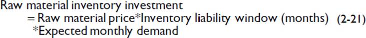
where the inventory liability window is the time during which the company takes ownership of inventory, and is calculated as
![]()
All the terms need to be expressed in the same time units (e.g., months). Since the raw material shipment schedule is weekly, the maximum cycle inventory is 7 days. The target safety stock is 1 month. Therefore, the maximum on-hand inventory is 37 days and the raw material inventory liability window is (37 – 30) = 7 days.
In this example, WIP inventory during the production process at the contract manufacturer also requires raw material for the duration of the lead time of 30 days. Therefore, this is added to the inventory liability window, resulting in a total value of (7 + 30) = 37 days = 1.23 month.
The raw material investment is calculated from Equation 2-21 as
Raw material inventory investment
= Raw material price ($5) * Inventory liability window (1.23 months)
* Expected monthly demand (10,000)
= $61,500.
Finished Goods Inventory
The finished goods inventory, priced at $10 per unit ($5 for raw material and $5 for labor) are in ABC Co.’s possession for the entire duration of the ocean shipment of 6 weeks. Therefore the inventory investment required is
Finished goods inventory investment
= Finished good ($10) * Inventory liability window (1.5 months)
* Expected monthly demand (10,000)
=$150,000.
Product Inventory at Distribution Center
The ocean carrier bills ABC Co. only after goods have been recovered; since the payment terms are Net 30, the liability window is -1 month. The maximum on-hand inventory is 1 month for cycle inventory plus 1 month for safety stock plus 1 month for receivables. Therefore, the liability window is (-1 + 1 + 1 + 1) = 2 months. The inventory budget requirement is calculated as
Product inventory investment
= Product at distribution center price ($12) * Inventory liability window (2 months)
* Expected monthly demand (10,000)
= $240,000.
The total inventory investment required is calculated by adding the investment for all the stages:
Inventory investment required
= Raw material inventory investment + Finished goods inventory investment
+ Product inventory investment
= $61,500 + $150,000 + $240,000
= $451,500.
Therefore, the current inventory budget of $360,000 is inadequate for maintaining adequate inventories and service levels for the supply chain.
The cash-to-cash cycle time is calculated as the days of inventory for the various stages plus the days receivables outstanding minus the days payables outstanding (Equation 2-23):
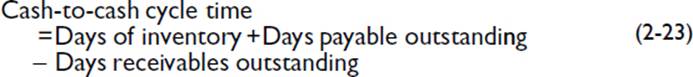
The cash-to-cash cycle time is equivalent to the addition of the liability windows for all the stages in the supply chain. In the example above, this would have resulted in 1.23 months for raw materials added to 1.5 months for finished goods and 2 months for products at the distribution, resulting in a cash-to-cash cycle time of 4.73 months. However, this measurement is not an accurate representation of the duration for which cash is tied up since the inventory investment is different for the different stages of the supply chain (for example, raw material inventory is priced lower than the product). Therefore, it is necessary to define a new measure of the liability, called the effective liability window, which is based on product costs,

For the example above, the effective liability window is calculated as
Effective liability window = $451,500/($10,000 * $12) = 3.76 months.
This value is lower than the previously calculated value of 4.73 months. The effective liability window is a more accurate representation of the true cash-to-cash cycle time and is a useful measure for product comparisons.
Inventory turns is yet another measure that is used to measure inventory investment and performance. Turns are calculated as
![]()
In the example, the expected sales are 10,000 unit per month, resulting in an annual cost of goods of (10,000 * $12/unit * 12 months) = $1,440,000. The average inventory is calculated as ($55,000 + $150,000 + $180,000) = $385,000, resulting in a computation of 3.7 turns.
None of these measurements—days of inventory, liability window, cash-to-cash cycle time, or inventory turns—is effective in conveying the benefit from holding inventory to the company. For example, it is difficult to respond to the question, “Are 3.7 turns too low? Should we increase turns? If so, what is the right value?” If safety stocks have been computed using the optimization procedures described previously, then these values can be assumed to be “right” for the supply chain. However, are other factors—such as manufacturing lead time, raw material commitments, and ocean transit time—resulting in an investment that does not provide an adequate return for the company? This question can be answered by computing the GMROI as

Therefore, the GMROI is a return-on-asset measurement for only the inventory investment. The expected gross margin is provided by the newsvendor model (Equation 2-13). The calculation procedure is as follows:
Continuation of Example 2-7 to describe the GMROI calculation.
The following additional data is collected for the products:
Expected monthly demand: 10,000 units.
Forecast error: 30%.
Expedite cost: $5 per unit.
Holding cost: $0.25 per month.
The product does not have a shelf-life.
From Equation 2-14, the optimal service level is calculated to be approximately 95%, and the optimal supply is (10,000 + 1.65*0.3*10,000) = 14,950 units. If it is possible to expedite inventory in order to satisfy demand in excess of inventory, then there is no lost demand. The expected sales per month = (10,000 * $20/unit) = $200,000; the expected expedited units is 59 units (from Equation 2-5); the cost of expediting is $5*59 = $296; the expected leftover inventory from Equation 2-8 is (14,950 - 10,000 - 50) = 5,009 units; and the holding cost is $0.25*5,009 = $1,252. Therefore, the expected gross profit is ($80,000 - $296 - $1,252) = $78,452.
From Equation 2-26, the GMROI is calculated to be
GMROI = (12 months * $78,452)/$451,500 = 2.08.
The GMROI of 2.08 indicates that $1 invested in inventory provides a return of $2.08 in one year.
The GMROI is a useful measure for gauging the efficiency of the supply chain in providing a return on the inventory asset. Note that this measure should not be confused with return on assets (ROA), which is a balance sheet measure that gauges the company’s ability to provide a return on all the company’s assets. The GMROI is a measurement of only the gross margin and inventory investment; any other charges that affect margin as well as investments required to operate the supply chain have not been included in this measurement. Therefore, while a low GMROI is an indicator of low ROA, a high GMROI by itself does not indicate a high ROA. (See Chapter 7 for additional discussions related to GMROI and other measures required to gauge the performance of the supply chain.)
Special Inventory Situations
The concepts presented in the previous sections were in the context of simple supply situations involving a single location and finished goods inventory. In reality, additional complexities can arise due to the myriad variations that are possible while creating the supply network and negotiating contracts with partners. A few such situations are described in the following sections.
Multiple Transportation Modes
The availability of multiple transportation modes allows for companies to utilize cost-effective options when time is available to meet demand, and more expensive expedite options when inventory levels are low. However, this same availability complicates the inventory decision, especially when the modes have widely differing batch sizes and costs. For example, an ocean container provides a low unit cost, but requires large quantities and longer transportation times. On the contrary, air shipments are faster and fewer units can be transported, but at a higher unit cost. Since goods are often transported based on a demand forecast, the cost trade-off between the different modes, holding costs, and margins is not trivial. A commonly employed strategy is to ship a bulk of the goods using the slower, lesser expensive mode, but to retain a minimal level of inventory close to the manufacturing location. Because not all the inventory is committed to the slower mode, it is possible to accommodate profitable rush orders if inventory situations become tight.
Yet another important situation arises for lifecycle products, as in the electronics and telecommunications industries. The products are characterized by demand volumes, prices, and forecast accuracy that vary considerably over the life of the product. It is common to segment the lifecycle of such products into phase. The first phase, product introduction, is characterized by high uncertainty in demand since the market acceptance for new products is unknown. At the same time, since the technology is new, it is possible to command a premium price and corresponding high margins as the company targets early adopters. Therefore, the inventory strategy is to maximize fill rates, resorting to air shipments if necessary to maintain target inventory levels. The second phase, product maturity, is characterized by steadier demand and predictability, a possible decrease in price as the novelty of the technology has worn off and the company is targeting the technology followers. In this phase, the strategy is to carefully manage inventories and costs to maximize margins. Use of air shipments is reserved for only firm orders, to ensure that inventory holding costs do not accrue. The final stage, product phase-out, happens when the market anticipates the next technology revision from the company. Demand rapidly drops off, and uncertainty is high related to the extent and speed with which it decreases. The company may have to reduce prices in order to spur demand, which increases margin pressures. There is a significant penalty related to leftover inventory, due to obsolescence. In this phase, inventory reduction and cost containment are the primary goals, and air shipments should be used infrequently, if at all. A summary of this policy is shown in Figure 2-15.
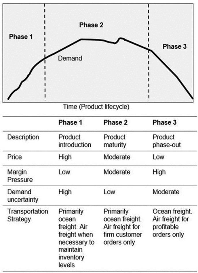
Figure 2-15. Example of a transportation mode strategy over the lifecycle of an electronic product
The approach described above can be used to analyze several other transportation situations, including full and partial truckloads and rail transport. Such a rigorous approach toward inventory analysis can result in effective use of multiple modes of transportation and an overall reduction in freight spend.
Staged Inventory
As the number of distribution and sales locations increase, so does the amount of inventory being held across the network, since each location holds safety stock to cover for variability. In such situations, staging inventory can reduce overall inventory levels without compromising service levels. Staging consolidates inventory at a central location, which has the effect of reducing demand variability, as exemplified in the excerpt below from an annual report of ScanSource, Inc. This lower variability results in lower safety stock and inventory levels. Additional savings are possible if holding costs are lower at the central facility as compared to more expensive local storage in metropolitan areas. Finally, as the number of products and locations grow, the benefit can further increase because the resources and investment required to operate in a decentralized manner can be prohibitive.
We operate a 600,000 square foot centralized distribution center in Southaven, Mississippi, which is located near the FedEx hub facility in Memphis, Tennessee and serves all of North America. Our European operation utilizes a centralized third-party warehouse located in Liege, Belgium that services all of Europe. Warehouses for our Latin American operations are located in Florida, Mexico, and Brazil. Our distribution model creates several advantages, including: (i) a reduced amount of “safety stock” inventory which, in turn, reduces the Company’s working capital requirements; (ii) an increased turnover rate through tighter controls over inventory; (iii) maintenance of a consistent order-fill rate; (iv) improved personnel productivity; (v) improved delivery time; (vi) simplified purchasing and tracking; (vii) decreased demand for management personnel; and (viii) flexibility to meet customer needs for systems integration. Our objective is to ship all orders on the same day, using barcode technology to expedite shipments and minimize shipping errors. The Company offers reduced freight rates and flexible delivery options to minimize a reseller’s need for inventory.
—ScanSource Inc., 2014 Annual Report
Clearly, there are many benefits provided by inventory staging and centralized distribution. However, staging is not without its drawbacks, and the applicability and returns need to be evaluated for each situation. Some of its general benefits and drawbacks are summarized in Table 2-5.
Table 2-5. Some Benefits and Drawbacks of Staging Inventory
|
Benefits |
Drawbacks |
|
Lower inventory investment |
Cost to set up new facilities |
|
Lower holding cost at central facility |
Limited inventory savings if demand across locations is correlated |
|
Lower cost due to transportation consolidation into central facility |
Additional transportation costs due to shipments from central to local facilities |
|
Higher service level if a few local facilities experience higher demand |
|
|
Lower replenishment times into local facilities |
Methods for estimating inventory requirements for the staged network can range from the simple and approximate, to complex methods that account explicitly for interactions between the different locations. An sample approach that extends the service level method is shown in Figure 2-16even though the formulation is developed for the simple case where demand and replenishment schedules are the same across the different locations, it is nevertheless useful for illustrating the benefit of staging. As expected, the magnitude of reduction in inventory increases with the number of local facilities. In addition, the benefits obtained from optimal placement of the central facility to reduce replenishment times can be compelling.
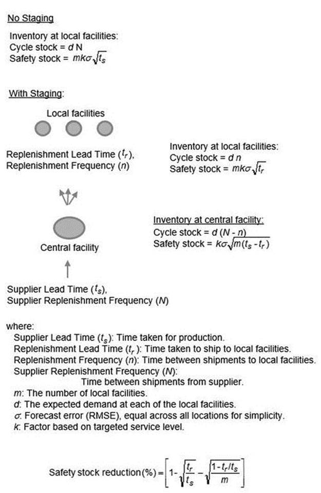
Figure 2-16. Inventories in a staged supply chain
Therefore, staging inventory is an effective strategy with the potential to reduce inventories without compromising service levels. Transportation implications need to be studied carefully before initiating staging, since routings will change. What was previously a single shipment from the supplier to each of the locations will now be delivered using two shipments—one from the supplier to the central facility, and another from the central facility to the location. It is not always necessary for staging to result in higher transportation levels—if the original shipments used expensive partial truckloads, staging can reduce costs with the use of less expensive full truckloads.
Finally, another factor that determines the effectiveness of staging is whether demand across the different locations is correlated. The analysis presented above assumed that demand is independent, as can be expected when the causes of demand are determined largely by the local environment. However, when demand is affected by non-local factors such as the economy or the introduction of competitive products, the same demand pattern may be experienced across multiple locations. This results in demand being correlated across multiple locations, which reduces the effectiveness of inventory aggregation.3
Raw Material Inventory
Raw materials are purchased parts and components that are required for production of one or more products. Raw materials are connected to products using a bill of material (BOM). Essentially, a BOM is a list of parts needed for a product. The concept of a BOM has been extended for several different situations. A BOM that captures the manufacturing steps and parts required for each stage is called a manufacturing BOM. A similar concept is the modular BOM, which describes sub-assemblies. An engineering BOM specifies parts used in the design, and a planning BOM is used for production planning or financial calculations. Planning bills are usually far simpler in structure and capture only essential information. An example is shown in Figure 2-17.
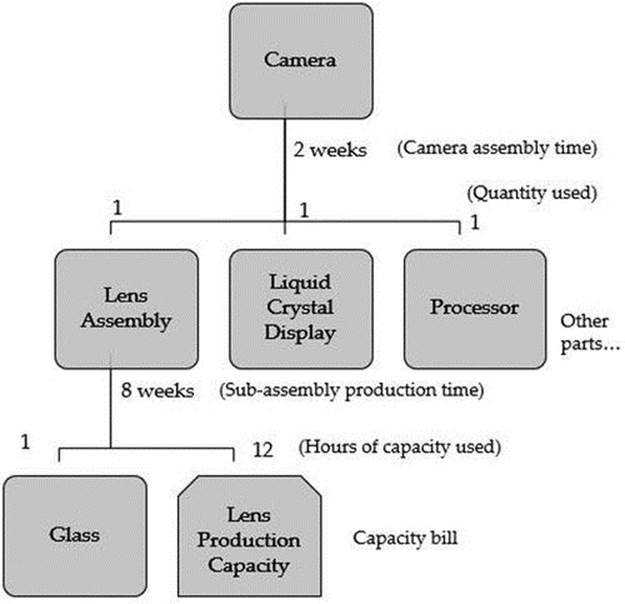
Figure 2-17. An example of a planning bill
Raw material inventory targets can be determined using the procedure described previously for staged inventory, which is illustrated in Figure 2-18. The planning bill is used to specify the interactions between the different products with the raw material; it collapses the several manufacturing steps into a single level and uses an estimate of the lead time for manufacturing for determining the finished goods and raw material safety stock.
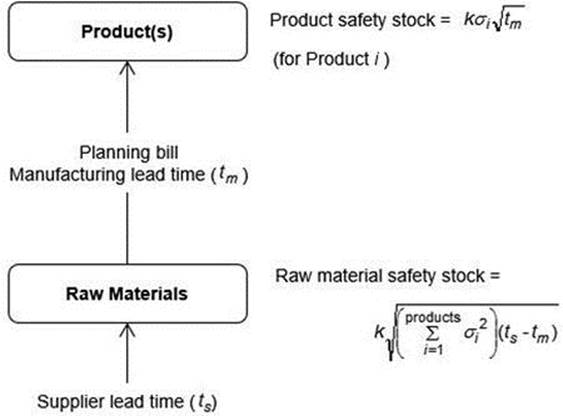
Figure 2-18. Inventory levels for raw materials
Holding raw material inventory is another example of staging. While distribution staging delays the commitment of inventory to a particular location, raw material inventory defers commitment to a particular product. The delay allows the forecast of each of the products to become clearer, ensuring that inventory and manufacturing labor are effectively utilized. As a result, the inventory benefits are similar to the case of staged inventory (Figure 2-18).
Postponement
Postponement is a strategy that delays the commitment of material to a final state (form or location) in order to provide a higher level of responsiveness and fulfillment, while simultaneously reducing inventory levels. This strategy is widely used in the automotive, aerospace, electronics, and apparel industries, although an increasing number of industries are adopting this strategy.4
An example of postponement most consumers are aware of comes from the paint industry. Where previously many hundreds or thousands of paint colors would need to be stocked to satisfy all color requests, it is now a common practice for the retailer to stock only the paint base and colorants separately, with the mixing of the two occurring during a sale to the consumer. This strategy is illustrated in Figure 2-19. The operational efficiency that is gained is clear—not only is it not necessary to stock hundreds of colors on the retailer’s shelves, but it is also not necessary to manufacture, transport, and store these different combinations. The result is a decrease in inventory levels at the distribution center and retail stores and a simultaneous increase in ability to satisfy almost any color combination a customer requests.
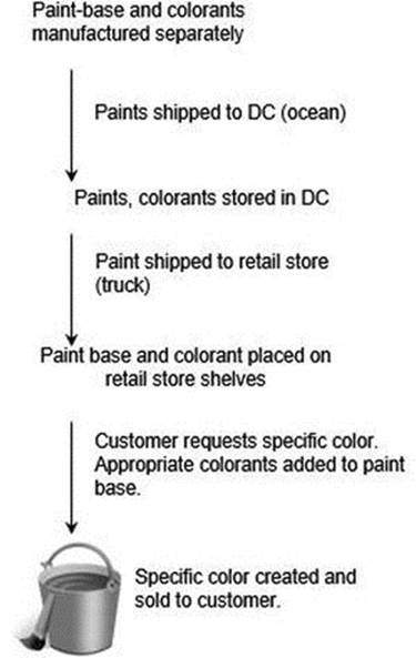
Figure 2-19. An illustration of postponement
Another example of postponement comes from the electronics industry with regard to the manufacturing of printers. Electronic goods often need to satisfy several country options related to language and power ratings. The traditional approach of stocking inventory for each of these options can result in high inventory levels and costly misses if demand for the country options is different from the forecast. In this case, the postponement strategy will result in printers being held in bulk and bundled with the appropriate country option prior to a shipment. This will result in lower overall inventory levels and lower re-packaging costs.
In general, postponement can be divided into two categories—manufacturing (and assembly) postponement and logistical postponement. Manufacturing postponement involves decisions made while the product is in production, the strategy being to develop a platform or module that allows for different configurations to be created with lower additional effort and cost, as emphasized in this excerpt from an annual report of PFSWeb, a provider of outsourced warehousing and fulfillment:
We will work with clients to re-sequence certain supply chain activities to aid in an inventory postponement strategy. We can provide kitting and assembly services and build-to-stock thousands of units daily to stock in a just-in-time (JIT) environment. This service, for example, can entail the procurement of packaging materials including retail boxes, foam inserts, and anti-static bags. These raw material components may be shipped to us from domestic or overseas manufacturers, and we will build the finished SKUs to stock for the client. Also included is the custom configuration of high-end printers and servers. This strategy allows manufacturers to make a smaller investment in base unit inventory while meeting changing customer demand for highly customizable products.
—PFSWeb, Inc., 2013 Annual Report
The retention of inventory in a raw form is an example of manufacturing postponement. Logistical postponement delays decisions related to packaging, labeling, and distribution. The staging of inventory is an example of logistical postponement.
Characteristics that make a product a good candidate for postponement include:
· The need for a large number of configurations in order to satisfy customer demand. This can be due to the nature of the product (for example, paint) or due to globalization and support for many languages and regional requirements (for example, printers).
· A high level of uncertainty in demand. The delay in the commitment of material to a finished form allows the demand picture to become clearer, resulting in lower inventories and higher fill rates.
· High holding costs, due to a high value of the product (for example, expensive electronic items), form factor (for example, bulky furniture), or short product lifecycles (for example, trendy music players).
· Long lead times, due to outsourced manufacturing and overseas transportation. The increase in lead time results in limited flexibility, which has to be offset using expensive inventory.
· The ability of a product to be customized with minimal expense, using a platform or modularization strategy.
The trade-off that needs to be considered in evaluating a postponement strategy is the benefit from holding less finished goods inventory against the possibility of increased cost due to transportation of assemblies and parts to the DC, as opposed to finished goods. The situation can be analyzed by calculating the total cost for the two cases separately, and comparing the incremental costs for manufacturing, transportation, and holding inventory. A simple comparison, assuming that supplier lead times are uniform across products and after postponement, is shown in Equation 2-27:
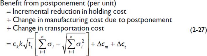
where
ck is the holding cost per period,
σ is the forecast error, expressed as a fraction of demand (i.e., the coefficient of variation, which results in the computation of unit costs),
ts is the supply lead time, and
Δc refers to incremental unit costs for manufacturing (m) and transportation (t).
Transportation costs can be lower if suppliers are closer to the point of postponement (closer to the point of sale) or if the base (unconfigured) unit and parts can be shipped in bulk at a lower cost. In such cases, reduced spend on transportation will further increase the benefit from postponement.
In general, the impact of postponement will not be restricted to a small section of the supply chain, but can impact material routings in manufacturing facilities and distribution centers. The cost comparison given in Equation 2-27 is far too simple and inadequate for such situation, instead a more comprehensive network-wide calculation of costs is required. Such methods are described in Chapter 6.
While postponement is a strategy that can provide companies with significant improvement opportunities, several challenges exist in identifying and implementing the strategy. These include the ability for a traditional company to rethink its approach to product design and fulfillment, the difficulty in quantifying and understanding the benefits, and inertia related to changing the supply chain to accommodate postponement. However, it appears to be only a matter of time before postponement practices become commonplace, due to adoption by market-leading companies and competitive pressures.
Supplier Flexibility
The need for companies to respond to changing market needs in order to compete effectively is at odds with the general trend toward outsourcing and off-shoring. This is the primary reason for the trend toward flexibility contracts between buyers and suppliers. Such contracts provide for short-term production flexibility for a price. While different industries have adopted different flavors, they can largely be categorized as time- or quantity-based flexibility.
Time-based flexibility, commonly referred to as blanket agreements or blanket orders, requires that the buyer commit to a total order quantity for a season. While a specified fraction of the total quantity is delivered at the beginning of the agreement period, the buyer may purchase the remaining quantity at a later date. Finally, the buyer pays a penalty for any units not purchased. In some cases, the penalty could be the full price of the part, as is sometimes the case in the semiconductor industry.
Quantity-based flexibility allows the buyer to vary order quantities based on a proportion of the original order. The procedure is that the buyer initially provides a forecast of purchases to the supplier. In subsequent periods, the buyer is allowed to change the orders and forecast within the limits specified by the flexibility contract. Usually, the flexibility provided is limited in the immediate period and gradually increases over time, as shown in Figure 2-20.
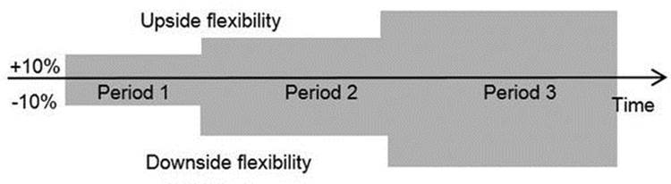
Figure 2-20. An illustration of a flexibility agreement with a contract manufacturer
The benefit provided by flexibility is enabling production adjustments based on a more accurate forecast in the short-term. Flexibility can also improve service levels since production can be increased in response to favorable market conditions. The benefits obtained from flexibility increase with demand variability. Specifically, the benefit from upside flexibility increases with increasing shortage costs and an aggressive approach to inventory levels. The benefit from downside flexibility increases with higher price erosion and holding costs.
There is an additional cost incurred by the supplier to provide flexibility, due to the need to maintain additional raw material or finished goods inventories, spare capacity, and changes to the production schedule. As a result, suppliers may be willing to provide flexibility if the additional price that can be charged is sufficient to cover the incremental costs. Similarly, the buyer will be willing to pay the additional price as long as the incremental benefit exceeds the cost.
The ability and willingness of a supplier to provide flexibility is dependent on the nature of the product and manufacturing operations. Situations that limit the ability to provide flexibility in the short term include:
· The use of custom parts, since the risk associated with high inventory levels increases.
· Complex manufacturing steps that require specialized labor, due to the time required to identify, hire, and train new resources.
· High factory utilization, since support for upside flexibility will require reliance on overtime or additional machinery.
· A sensitive labor environment, such as a unionized workforce, that limits the ability to lower production.
Conversely, other situations allow the supply chain to be more flexible:
· Low factory utilization, since an increase in production can be supported and will increase the profitability of the plant.
· A supplier with a diversified customer and product portfolio, since production increases and decreases can be absorbed by other product lines.
· Use of mass-produced components (as opposed to custom parts) that are inexpensive to stock or can be used across multiple products.
· Manufacturing operations that are of low or moderate complexity, so that additional resources can be added quickly.
· Easy availability of labor and a flexible labor force.
In conclusion, supply flexibility can be an effective method for improving margins and service levels for products that display moderate to high uncertainty in demand. In order for effective use of this strategy, both parties need to implement appropriate processes to ensure that the guidelines and requirements are being followed.
Correlated Demand
Most of the situations described in the previous sections assume that demand is independent across the different time periods. When this is not the case, the safety stock requirement is calculated as
![]()
where n is the number of periods for which demand is perfectly (positively) correlated, and demand and supply variances are independent. Since the beneficial effect of reducing variance when demand is independent is lost, the resulting safety stock levels are higher. The impact of the additional inventory on margins is similar to the effect discussed for supply variability (Figure 2-11).
Correlated demand can occur due to several reasons, including the following:
· Economic shifts that cause sustained up- or down-trends in demand. These economic factors can include changes in interest rates, a housing market collapse or surge, and even changes in a country’s regulations.
· Competitive activity, including the introduction of new products that have the capability to fundamentally change demand patterns. Note that the competition’s promotional activity does not have the same impact since prices revert to original quantities after a duration, resulting in a return to equilibrium for the product.
· Introduction of large business customers who can increase demand for several months at a stretch. Similarly, the loss of large customers can have the effect of decreasing demand for several months.
· Introduction of new products for which consumer perception is unclear. The first few months of sales can display consistent up- or down-trends based on the market’s response.
· Cannibalization of demand due to additional sales of other products in the portfolio.
In addition, even though demand may be independent for several months at a stretch, correlation can occur due to any one of the factors described above. Indeed, it is not clear when such factors will surface, which increases the challenge of planning inventories. If inventory levels are set based on an assumption of independent demand, it is easy to see why supply chain “surprises” and high levels of expedites or inventories can occur.
EXAMPLE 2-8: EFFECT OF CORRELATED DEMAND ON INVENTORY LEVELS
An electronic product displays a forecast error of 25% (relative to the expected monthly demand), a supply variability of 10 days, and a supply lead time of 2 months.
If the desired service level is 97%, the safety stock is calculated from Figure 2-5 for the independent demand case as
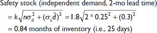
On the other hand, if demand is perfectly (positively) correlated, safety stock is calculated as
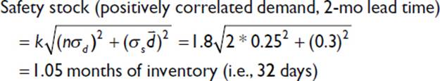
It is clear that the effect of correlation is to increase inventory levels in order to provide a targeted service level. If lead times are large, the impact of correlated demand is magnified, as shown in Table 2-6.
Table 2-6. Impact of Demand Correlation on Inventory Levels
|
Supply Lead Time |
Safety Stock for Independent Demand |
Safety Stock for Dependent Demand |
|
2 months |
35 days |
46 days |
|
3 months |
41 days |
67 days |
|
4 months |
46 days |
88 days |
Finally, if there is reason to believe that a certain level of correlation exists between demand and supply variability, these inventory requirements will further increase, as explained previously in the derivation of the service level method.
Summary
The chapter introduced several important concepts regarding the importance of inventory for a business and the different methods available to the analyst to ensure that margins and profits are adequately considered in the decision-making process. While the success of the inventory strategy depends on the processes and systems put in place, an equally important factor is the role of the analyst. The analyst has the challenging task of managing uncertainty and balancing the constant demand for inventory from the rest of the organization against the cost of excesses.
One of the important steps that drives the effectiveness of the inventory plan is defining safety stock requirements. Several methods have been introduced in this chapter, each with its advantages and disadvantages, and applicability to different situations. Since the choice of methods can be confusing, a simple set of guidelines has been provided in Table 2-7. It is important to recognize that these industry-specific guidelines are approximate. Products in any of these categories can briefly or permanently display characteristics that make it well-suited for other methods. Therefore, it is important that the inventory analyst gain an understanding of the different inventory categories and management methods.
Table 2-7. Some Guidelines for Using Different Inventory Models
|
Product |
Situation |
Appropriate Method |
|
Groceries |
Limited shelf-life, high obsolescence rate |
Newsvendor model |
|
Consumer staples |
Steady price, low obsolescence cost |
Service level method if shortage costs are low, else incremental margin model |
|
Electronics |
Significant price changes, lifecycle products |
Incremental margin model |
|
Consumer durables |
High holding and shortage costs |
Incremental margin model |
Choosing the appropriate method merely improves the quality of the guidance provided. Given that several assumptions have been made while constructing these models, this guidance needs to be modified based on the analyst’s knowledge of out-of-bounds or special situations. The use of control limits (that is, upper and lower bands for maintaining inventory) is recommended for ensuring that small changes in underlying variables do not disrupt the performance of the supply chain.
When several hundreds or even thousands of items have to be managed, it is easy to overlook poor performance and incur additional costs. Therefore, it is important to implement a rigorous performance review process that identifies poorly performing items (further discussed in Chapter 7).
In many situations, it is not easy to calculate service levels and fill rates accurately due to loss of information during the sales process. For example, if a salesman is aware of low inventory levels for a particular product and guides a customer toward the purchase of an alternative product, metrics based on sales data will fail to capture this shortfall. In fact, the data can lead the inventory analyst to believe that the inventory planning process is performing well, which can be contrary to the belief of the rest of the organization and the company’s customers. In such situations, it is necessary to augment the quantitative measurement with surveys and interviews with the sales and marketing division and channel customers—any perception that a particular product is always in short supply needs to be considered while setting inventory parameters and safety stock levels.
________________
1For further details and guidelines for the use of other probability functions, see for example Athanasios Papoulis, Random Variables and Stochastic Processes (McGraw Hill, 1989).
2See, for example, Erwin Kreyzig, Advanced Engineering Mathematics (John Wiley, 2005).
3When demand is independent, the RMSE of forecast error for the central facility is calculated as ![]() , where σ is the standard deviation of forecast error for each of the m facilities. However, when demand is not independent, the relationship is if perfectly correlated, and the beneficial effect of aggregation is lost.
, where σ is the standard deviation of forecast error for each of the m facilities. However, when demand is not independent, the relationship is if perfectly correlated, and the beneficial effect of aggregation is lost.
4Susan M. Rietze, “Case Studies of Postponement in the Supply Chain,” Department of Civil and Environmental Engineering, Massachusetts Institute of Technology, 2006.
All materials on the site are licensed Creative Commons Attribution-Sharealike 3.0 Unported CC BY-SA 3.0 & GNU Free Documentation License (GFDL)
If you are the copyright holder of any material contained on our site and intend to remove it, please contact our site administrator for approval.
© 2016-2026 All site design rights belong to S.Y.A.